A new approach to LST modeling and normalization under clear-sky conditions based on a local optimization strategy

ABSTRACT

The normalization of LST relative to environmental parameters is of great importance in various environmental applications. The purpose of this study was to develop a new approach for LST normalization relative to environmental variables. These included topographic variables (i.e. solar irradiance and near-surface temperature lapse rate (NSTLR)) as well as biophysical properties (i.e. vegetation, wetness, and albedo). The study was conducted in two phases, namely (1) using global and (2) local optimization strategies to calculate the regression coefficients of environmental variables in the partial least squares regression (PLSR) and build the non-linear linking model in the random forest regression (RFR). The RMSEs between actual LST and modeled LST based on the global and local optimization strategies using PLSR (RFR) were 2.202 (0.935) and 0.939 (0.835) °C, respectively. The results showed that RFR had higher efficiency than PLSR in normalizing LST. Moreover, the local optimization method outperformed the global optimization method in terms of normalization accuracy. The results of this study could be very useful in many environmental applications such as identifying thermal anomalies, and surface anthropogenic heat island modeling.

KEYWORDS:

• Normalization
• land surface temperature
• environmental variables
• partial least squares
• random forest
• local strategy

1. Introduction

Land surface temperature (LST) is one of the critical variables in comprehending earth surface-related processes (Li et al. 2013; Firozjaei, Kiavarz, and Alavipanah 2022a). LST plays an important role in studies on ground resources (Mansor et al. 1994; Jia et al. 2017), environmental variables (Alavipanah, Kiavarz, and Firozjaei 2017; Firozjaei et al. 2018), surface energy balance (SEB) (Friedl 2002; Weng et al. 2019), geological structure (Ma et al. 2010), climate change (Voogt and Oke 2003; Berger et al. 2017), water resources (Anderson et al. 2012), soil moisture (Han, Wang, and Zhao 2010), evapotranspiration (Harris et al. 2017; Lievens et al. 2017), energy consumption (Giridharan and Emmanuel 2018), and thermal comfort (Mijani et al. 2019). In recent decades, LST regimes are regularly acquired over a large geographic area using thermal remote sensors that operate in the more extended wavelength region of the electromagnetic spectrum. LST regimes are mainly influenced by a set of environmental variables such as geographical location (e.g. longitude and latitude), temporal position (e.g. hours per day and days in year), and topographic condition (e.g. elevation, slope, aspect, and shadow). The intrinsic thermal characteristics (e.g. thermal inertia and emissivity), surface biophysical characteristics (e.g. moisture, vegetation, brightness, albedo, and evapotranspiration), synoptic and climate variables (e.g. wind, air pressure, and water vapor in the atmosphere), and sub-ground conditions (e.g. geothermal, hydrothermal, fault and volcanic areas) can also cause heterogeneous distribution of the LST (Coolbaugh et al. 2007; Gutiérrez et al. 2012; Mattar et al. 2014; Malbéteau et al. 2017; Weng et al. 2019; Zhao et al. 2019; Zhao et al. 2019; Firozjaei, Kiavarz, and Alavipanah 2022b).

The normalization of LST relative to environmental parameters is of great importance when it comes to increasing the accuracy of modeling various parameters in some environmental applications (Coolbaugh et al. 2007; Mattar et al. 2014; Malbéteau et al. 2017; Zhao et al. 2019; Firozjaei et al. 2020; Firozjaei et al. 2020). For example, in the process of calculating the near-surface temperature lapse rate (NSTLR) value for a region based on satellite data, only the amount of LST changes due to the change in elevation should be taken into account. Therefore, the normalization of LST relative to environmental parameters except for elevation can cause a significant increase in the accuracy of NSTLR calculation. In addition, the normalization of LST relative to environmental parameters can increase the accuracy of identifying thermal anomalies caused by fires, volcano activity, faults, and geothermal resources based on satellite data. The accuracy of estimating the amount of thermal energy loss from the roof of buildings in the urban environment based on satellite thermal images can be increased by considering LST normalization relative to the geometric characteristics of the urban structure, the effect of solar radiation, and the surface biophysical characteristics. In another application, the normalization of LST relative to environmental parameters allows for a more accurate estimation of anthropogenic heat flux and the resulting heat island in the urban environment. As a result, it is of great importance to develop and provide appropriate strategies for normalizing LST relative to environmental parameters.

Previous studies have directly and indirectly addressed LST normalization relative to the environmental variables. Hassan et al. (2007) presented a new approach to model surface wetness in humid regions with heterogeneous topography based on a temperature-vegetation wetness index (TVWI). They normalized terrain-induced effects in satellite-derived LST to improve the model of surface wetness in areas with high elevation by applying vertical atmospheric pressure on LST based on DEM data. Verhoest et al. (2012) used characteristics of the relationship between LST and vegetation index to evaluate the evaporation and transpiration status in a mountainous region under heterogeneous topographic conditions. Their results indicated that the error in NSTLR modeling based on the LST-DEM feature space was decreased with the normalization of LST relative to the vegetation index. Malbéteau et al. (2017) presented models including dual-source surface energy balance (dual-SEB), the slope of dry edges, and multi-linear regression for LST normalization relative to the topography effects in a mountainous region. The results demonstrated that the dual-SEB model was more efficient in LST normalization compared to other models. Zhao et al. (2019) developed a normalization approach based on random forest regression (RFR) to normalize LST relative to the topography effect. The validation of the results made it clear that this approach had an obvious advantage of normalizing the topography effect on the spatial variation of LST over the study area. Weng et al. (2019) presented a triple-source surface energy balance (triple-SEB) model to normalize LST. They concluded that the triple-SEB model outperformed the dual-SEB model in normalizing surface temperature. Comparing the performance of the LST-DEM and normalized LST-DEM feature spaces in calculating NSTLR, Firozjaei et al. (2020) used a regression model to normalize LST relative to surface characteristics. Their study results showed that the use of normalized LST-DEM feature space increased the accuracy of NSTLR modeling compared to the LST-DEM feature space. Firozjaei et al. (2020) used normalized LST obtained from the triple-source surface energy balance (triple-SEB) to model LST relative to anthropogenic heat flux and surface anthropogenic heat island (SAHI) intensity. The results showed that the use of the triple-SEB model for LST normalization increased the accuracy with respect to anthropogenic heat flux and SAHI in different conditions.

Only a few models have so far been developed for normalizing LST relative to environmental parameters. In general, these models can be classified into two groups (1) regression models and (2) models based on surface energy balance. To implement the surface energy balance model, a lot of additional information is needed to form and solve the equations of different components of the surface energy balance; hence the complexity of implementing these types of models is high. The processing volume and time required for building models based on surface energy balance are high. Regression models are less complicated to implement than surface energy balance models. However, the implementation of regression models presented in previous studies was based on global optimization. In other words, global optimization is used to solve the unknown coefficients of each of the environmental parameters in the regression model, and a constant value is calculated for each of the unknown coefficients for the whole study area. Some have challenged the effectiveness of regression approaches with global optimization for LST modeling and normalization in heterogeneous regions in terms of surface characteristics. Because the amount and type of influence of each environmental parameter on LST can be different in regions with different conditions. Therefore, in this study, a regression model with a local optimization approach is proposed for LST normalization.

Concerning the strengths and weaknesses of previous studies, the formulation of our objectives is two-fold. Firstly, we opted to quantify the impact of a set of environment variables including incident solar radiation, albedo, elevation, vegetation, wetness, and surface relief conditions on the satellite-derived LST regimes. Secondly, we presented a regression model with a local optimization strategy to normalize the effect of a set of environment variables on the satellite-derived LST and validate the results. The validation was carried out based on LST measured by ground devices.

2. Study area

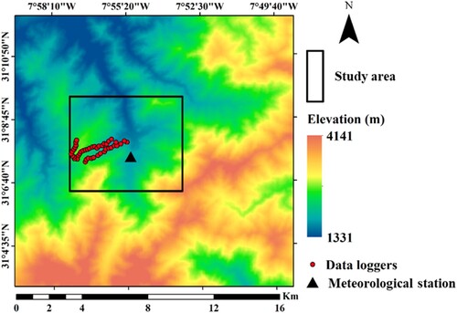
For the implementation of the LST modeling and normalization model, a rugged region (47.72 km²) was selected as the study area. This region is located in the Imlil valley in the Moroccan mountain chain (31°06′10″ to 31°09′37″ latitude N and 07°57′42″ to 07°53′02″ longitude W). The spatial and temporal distribution of the topographical and biophysical characteristics of the study area is heterogeneous. The elevation varies from 1583 to 3660 m, the slope from 0 to 69 degrees, and the aspect from 0 to 359.6 degrees. The average highest and lowest air temperatures in the study area are 26°C and 12°C, respectively. The average relative humidity, the rainfall level, and the average wind speed are respectively measured at 63%, 600 mm/year, and 2.5 m/s in this area. The land cover of the study area includes built-up, bare soil, agriculture and green space classes. Vegetation density and soil moisture in the central areas of the study area are higher than other areas. Due to the heterogeneity of environmental conditions and the availability of LST derived from ground devices at satellite overpass time, this region was selected to implement and assess the proposed LST modeling and normalization model. The geographic location of the study area is shown in Figure 1.

Figure 1. The geographic location of the study area and data loggers specifically measuring the soil temperature.

3. Materials and methods

3.1. Data and pre-processing

The research data included Landsat 8 satellite imagery (Path: 202, Row: 038) for 24/05/2014, 25/06/2014, 27/07/2014, and 12/08/2014, Global Digital Elevation Model (GDEM) with a resolution of 30 meters, and MOD07 water vapor product at the Landsat 8 satellite overpass time (Table 1). The data are available on the US Geological Survey website (http://www.usgs.gov) and NASA’s website (https://ladsweb.nascom.nasa.gov).

Table 1. Specifications of data used in this study.

Data type	Satellite/ Sensor	Spatial resolution	Date of satellite imagery acquisition	Source
Satellite images (day)	Landsat 8 (OLI/TIRS)	30 m	24/05/2014, 25/06/2014, 27/07/2014 and 12/08/2014	http://www.usgs.gov
Water vapor (MOD07)	MODIS	5000 m	Same of Landsat satellite overpass time	https://ladsweb.nascom.nasa.gov
Global Digital Elevation Model (GDEM)	ASTER	30 m	2011	https://www.earthdata.nasa.gov/
Soil temperature	Ground device	——	Same of Landsat satellite overpass time	–

The Landsat 8 satellite was launched on 11 February 2013, which has two main sensors, namely Operational Land Imager (OLI) and Thermal Infrared Sensor (TIRS). The OLI sensor collects images using nine spectral bands at different wavelengths of visible, near-infrared, and shortwave with a resolution of 30 meters. TIRS bands of Landsat 8 are acquired at the 100-meter resolution but resampled to the 30-meter resolution by the cubic convolution method. The cubic convolution uses a cubic transform to interpolate between the control points of known geographical positions to find the geographical coordinates of pixels in the input image. For each pixel in the output image, the algorithm calculates a weighted average of the sixteen closest input pixels and transfer this to the new image. The obtained Landsat images from the USGS included the Level-1 Precision Terrain (L1TP) data. The geo-registration was consistent and an RMSE ≤0.5 pixels was achieved (Weng et al. 2019).

The Moderate Resolution Imaging Spectroradiometer (MODIS) atmospheric water-vapor product (MOD07 with a resolution of 5000 meters) is an estimate of the total tropospheric column water vapor made of integrated MODIS infrared retrievals of atmospheric moisture profiles in clear scenes. This product was used to complete the input variables of LST obtained from satellite imagery. Moreover, GDEM produced by Japan and the United States National Aeronautics and Space Administration (NASA) was used for modeling the NSTLR effect and the solar irradiance with absolute horizontal and vertical accuracies of 30 and 17 m. The GDEM covers the earth's surface between 83°S and 83°N latitudes (Tachikawa et al. 2011).

To evaluate the accuracy of the modeled LST, the ground device-derived LST was used at the satellite overpass. The DS1921G model of temperature recorder was used in the present study. This device records the soil temperature in the range of −30 to −70 °C with an accuracy of 1°C. In 2014, a total of 41 devices were studied for the MIXMOD-E (ANR-13-JS06-0003-01) and REC (RISE-2014-645642-REC) projects at a depth of 1 cm in the soil (Malbéteau et al. 2017). The ground device-derived LST was continuously recorded for a period of 6 months. The location of ground-based devices is shown in Figure 1.

3.2. Methods

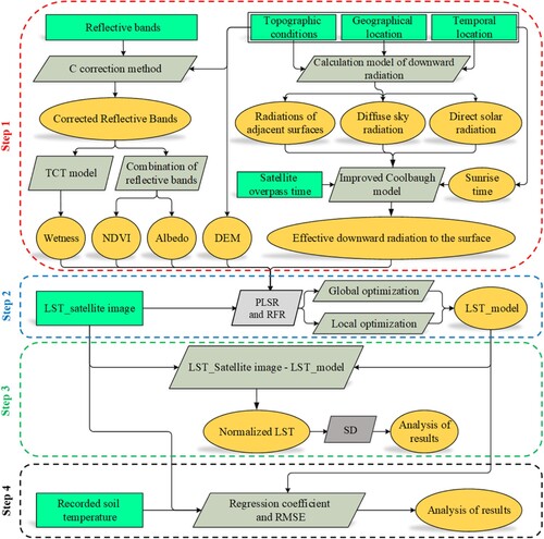
In the present study, in the first step, LST and environmental variables affecting LST such as effective cumulative solar irradiance, vegetation, NSTLR, albedo, and surface wetness were calculated for different dates. In the second step, partial least squares regression (PLSR) and RFR coefficients were calculated using two global and local optimization strategies for each date. In the third step, LST was normalized relative to environmental variables using observed LST and modeled LST. In the fourth step, to evaluate the accuracy of different modeling results, the RMSE and determination coefficients were calculated between modeled LST and LST obtained from Landsat 8 imagery, as well as between modeled LST and LST obtained from ground devices. In addition, the standard deviation of normalized LST values was estimated and analyzed. The proposed model for LST normalization is shown in Figure 2.

Figure 2. The proposed conceptual model for LST normalization.

3.2.1. Modeling of environmental variables

3.2.1.1. Solar radiation and topographic variables

There are two approaches to modeling the solar and topographic effects on LST. The first approach considers the effect of instantaneous solar irradiance on LST. Instantaneous solar irradiance is the amount of incoming radiation to the earth's surface at the satellite overpass time. The second approach considers the effect of solar irradiance on LST from the sunrise to the satellite overpass time. In this study, based on the second approach, the solar irradiance was modeled on the spatial distribution of LST. The improved Coolbaugh model was proposed to model the effect of solar irradiance on LST. Coolbaugh et al. (2007) proposed a model for investigating the solar irradiance effect from the sunrise to the satellite overpass time as a discrete cumulative relation as shown by Eq. (1)(1) $\mathrm{Rg}=S_0\sum _t(M({\alpha }_t)\cos ({\theta }_t)D_t)\mathrm{\Delta }t$(1) . (1) $\mathrm{Rg}=S_0\sum _t(M({\alpha }_t)\cos ({\theta }_t)D_t)\mathrm{\Delta }t$(1) In Eq. (1)(1) $\mathrm{Rg}=S_0\sum _t(M({\alpha }_t)\cos ({\theta }_t)D_t)\mathrm{\Delta }t$(1) , $\mathrm{Rg}$ is the total amount of discrete cumulative solar irradiance, $S_0$ is the solar radiation constant, $M({\alpha }_t)$ is the atmospheric transmissivity of the solar zenith angle at time t, ${\alpha }_t$ is the solar zenith angle at time t, ${\theta }_t$ is the local incidence angle of the solar beam on the surface at time t, $D_t$ is the delay factor and, $\mathrm{\Delta }t$ is the time interval for calculating the solar irradiance (i.e. one hour in the Coolbaugh model). In the Coolbaugh model, the solar effect on the heating of the earth is calculated as a discrete cumulative relation. Meanwhile, it is important to notice that the land surface continuously receives solar energy from sunrise until sunset. For this reason, in the model presented in this study, the solar and topographic effects on LST are calculated as continuous cumulative variables. The Coolbaugh model only accounts for the direct solar radiation (Coolbaugh et al. 2007), however, the improved Coolbaugh model factors in both direct and diffuse solar radiation as well as the radiation reflected by adjacent surfaces. The effective cumulative solar irradiance is computed as continuous cumulative values using the improved Coolbaugh as in Eq. (2)(2) $\mathrm{CRg}=S_0\underset{t_1}{\overset{t_2}{\int }}(((G_{Bt}+G_{Dt}+G_{Gt}){)}_t{D}_t)dt$(2) . (2) $\mathrm{CRg}=S_0\underset{t_1}{\overset{t_2}{\int }}(((G_{Bt}+G_{Dt}+G_{Gt}){)}_t{D}_t)dt$(2) With CRg being the total amount of effective cumulative solar irradiance, $t_1$ sunrise time (Allen, Trezza, and Tasumi 2006), $t_2$ satellite passage, $G_{Bt}$ direct solar radiation (Kalogirou 2013), $G_{Dt}$ diffuse sky radiation (Tachikawa et al. 2011), $G_{Gt}$ reflected radiations from the adjacent surfaces (Proy, Tanre, and Deschamps 1989; Merlin and Chehbouni 2004; Mousivand et al. 2015), and $D_t$ is the delay factor (Gutiérrez et al. 2012) of the Coolbaugh model.

3.2.1.2. NSTLR variable

In a troposphere, assuming a constant time and geographical location, air pressure decreases as altitude increases. This is an adiabatic process in which there is a reduction in internal air energy and a drop in air temperature (Jacobson 2005). This is suggestive of the effect of NSTLR, most evident at night and influenced by solar and topographic effect variables in daytime (Firozjaei et al. 2020). Theoretically, the NSTLR value is about 9.8°C km⁻¹ under adiabatic arid conditions, about 6-7°C km⁻¹ under adiabatic semi-arid conditions at lower elevations than 10 km, and about 3.6°C km⁻¹ under adiabatic wet conditions (Danielson, Levin, and Abrams 2003; Rolland 2003; Minder, Mote, and Lundquist 2010). Practically, NSTLR should be estimated according to the time and geographical location (Danielson, Levin, and Abrams 2003; Rolland 2003; Minder, Mote, and Lundquist 2010). Accordingly, GDEM was used in the proposed model for modeling NSTLR (Boudhar et al. 2011).

3.2.1.3. Surface biophysical properties

In order to model the surface biophysical properties, Landsat reflective bands were used based on the spectral behavior of each biophysical property. At first, the reflective bands were corrected relative to topography and shadow effects. The values of reflective bands were then corrected by the developed C correction method (Hantson and Chuvieco 2011) relative to the effects of topography and shadow.

a)	Vegetation

One of the environmental variables affecting LST is surface vegetation density. Normally, LST reduces with the increase in surface vegetation (Amiri et al. 2009; Zhang, Odeh, and Han 2009; Karnieli et al. 2010; Firozjaei et al. 2018). In this study, the NDVI was used for modeling vegetation using Eq. (3)(3) $\mathrm{NDVI}={\displaystyle \frac{\mathrm{Re}{\mathrm{f}}_5-\mathrm{Re}{\mathrm{f}}_4}{\mathrm{Re}{\mathrm{f}}_5+\mathrm{Re}{\mathrm{f}}_4}}$(3) (Tucker 1979). (3) $\mathrm{NDVI}={\displaystyle \frac{\mathrm{Re}{\mathrm{f}}_5-\mathrm{Re}{\mathrm{f}}_4}{\mathrm{Re}{\mathrm{f}}_5+\mathrm{Re}{\mathrm{f}}_4}}$(3) In Eq. (3)(3) $\mathrm{NDVI}={\displaystyle \frac{\mathrm{Re}{\mathrm{f}}_5-\mathrm{Re}{\mathrm{f}}_4}{\mathrm{Re}{\mathrm{f}}_5+\mathrm{Re}{\mathrm{f}}_4}}$(3) , $\mathrm{Re}{\mathrm{f}}_5$ and $\mathrm{Re}{\mathrm{f}}_4$ are the corrected ground reflectance of near-infrared and red bands, respectively.

b)

Wetness

Tasseled cap transformation (TCT) takes different linear combinations of satellite imagery reflective bands and a specific coefficient matrix to obtain valuable information on surface biophysical properties. Greenness, brightness, and wetness information were extracted from TCT band combinations. The wetness information content affects the characteristics related to water, soil, vegetation, and built-up land moisture (Liu et al. 2015). The coefficients for TCT combination of Landsat 8 imagery used for calculating the surface wetness are shown in Eq. (4)(4) $\mathrm{Wetness}=0.1115\mathrm{Re}{\mathrm{f}}_2+0.1973\mathrm{Re}{\mathrm{f}}_3+0.3283\mathrm{Re}{\mathrm{f}}_4+0.3407\mathrm{Re}{\mathrm{f}}_5-0.7117\mathrm{Re}{\mathrm{f}}_6-0.4559\mathrm{Re}{\mathrm{f}}_7$(4) (Liu et al. 2015). (4) $\mathrm{Wetness}=0.1115\mathrm{Re}{\mathrm{f}}_2+0.1973\mathrm{Re}{\mathrm{f}}_3+0.3283\mathrm{Re}{\mathrm{f}}_4+0.3407\mathrm{Re}{\mathrm{f}}_5-0.7117\mathrm{Re}{\mathrm{f}}_6-0.4559\mathrm{Re}{\mathrm{f}}_7$(4) In Eq. (4)(4) $\mathrm{Wetness}=0.1115\mathrm{Re}{\mathrm{f}}_2+0.1973\mathrm{Re}{\mathrm{f}}_3+0.3283\mathrm{Re}{\mathrm{f}}_4+0.3407\mathrm{Re}{\mathrm{f}}_5-0.7117\mathrm{Re}{\mathrm{f}}_6-0.4559\mathrm{Re}{\mathrm{f}}_7$(4) , $\mathrm{Re}{\mathrm{f}}_2$, $\mathrm{Re}{\mathrm{f}}_3$, $\mathrm{Re}{\mathrm{f}}_4$, $\mathrm{Re}{\mathrm{f}}_5$, $\mathrm{Re}{\mathrm{f}}_6$ and $\mathrm{Re}{\mathrm{f}}_7$ are are the corrected ground reflectance of blue, green, red, near-infrared, shortwave inferered 1 and shortwave inferered 2 bands, respectively.

• c) Surface albedo

Numerous studies have investigated the effect of albedo on LST (Vlassova et al. 2014). The linear combination of Landsat 8 reflective bands was used to estimate the albedo (Eq. (5)(5) $\mathrm{Albedo}=0.356\mathrm{Re}{\mathrm{f}}_2+0.130\mathrm{Re}{\mathrm{f}}_3+0.373\mathrm{Re}{\mathrm{f}}_4+0.085\mathrm{Re}{\mathrm{f}}_5+0.072\mathrm{Re}{\mathrm{f}}_6+0.072\mathrm{Re}{\mathrm{f}}_7-0.0018$(5) ) (Silva et al. 2016). (5) $\mathrm{Albedo}=0.356\mathrm{Re}{\mathrm{f}}_2+0.130\mathrm{Re}{\mathrm{f}}_3+0.373\mathrm{Re}{\mathrm{f}}_4+0.085\mathrm{Re}{\mathrm{f}}_5+0.072\mathrm{Re}{\mathrm{f}}_6+0.072\mathrm{Re}{\mathrm{f}}_7-0.0018$(5) In Eq. (5)(5) $\mathrm{Albedo}=0.356\mathrm{Re}{\mathrm{f}}_2+0.130\mathrm{Re}{\mathrm{f}}_3+0.373\mathrm{Re}{\mathrm{f}}_4+0.085\mathrm{Re}{\mathrm{f}}_5+0.072\mathrm{Re}{\mathrm{f}}_6+0.072\mathrm{Re}{\mathrm{f}}_7-0.0018$(5) , $\mathrm{Re}{\mathrm{f}}_2$, $\mathrm{Re}{\mathrm{f}}_3$, $\mathrm{Re}{\mathrm{f}}_4$, $\mathrm{Re}{\mathrm{f}}_5$, $\mathrm{Re}{\mathrm{f}}_6$ and $\mathrm{Re}{\mathrm{f}}_7$ are are the corrected ground reflectance of blue, green, red, near-infrared, shortwave inferered 1 and shortwave inferered 2 bands, respectively.

3.2.2. LST calculation

Single Channel (SC) (Jiménez-Muñoz et al. 2014; Yu, Guo, and Wu 2014), Improved Mono-Window (IMW) (Wang et al. 2015), and Split Window (SW) (Jiménez-Muñoz et al. 2014) algorithms were used to calculate LST. Band 10 of Landsat 8 was employed to calculate LST using SC and IMW algorithms (Barsi et al. 2014). In this study, the land surface emissivity (LSE) was calculated using the NDVI threshold model (Jimenez-Munoz et al. 2014; Yu, Guo, and Wu 2014). The accuracy of LST derived from each algorithm was assessed using LST obtained from ground devices at the satellite overpass time. Finally, according to the results of accuracy evaluation of different methods for each date, the best LST map was selected to be used for the normalization stages.

3.2.3. Proposed model for LST modeling and normalization

Equations 6–9 have been suggested for LST modeling and normalization relative to the environmental variables as linear combination.

For pixel $(i,j)$: (6) $\mathrm{NLS}{\mathrm{T}}_{\mathrm{GPLS}}(i,j)=\mathrm{LST}(i,j)-\mathrm{LS}{\mathrm{T}}_{\mathrm{modelGPLS}}(i,j)$(6) (7) $\mathrm{LS}{\mathrm{T}}_{\mathrm{modelGPLS}}(i,j)=a_1((1-\mathrm{Albedo}(i,j))\times \mathrm{CRg}(i,j))+a_2(\mathrm{DEM}(i,j))+a_3(\mathrm{NDVI}(i,j))+a_4(\mathrm{Wetness}(i,j))$(7) (8) $\mathrm{NLS}{\mathrm{T}}_{\mathrm{LPLS}}(i,j)=\mathrm{LST}(i,j)-\mathrm{LS}{\mathrm{T}}_{\mathrm{modelLPLS}}(i,j)$(8) (9) $\mathrm{LS}{\mathrm{T}}_{\mathrm{modelLPLS}}(i,j)=a_1(i,j)((1-\mathrm{Albedo}(i,j))\times \mathrm{CRg}(i,j))+a_2(i,j)(\mathrm{DEM}(i,j))+a_3(i,j)(\mathrm{NDVI}(i,j))+a_4(i,j)(\mathrm{Wetness}(i,j))$(9)

Where $\mathrm{LS}{\mathrm{T}}_{\mathrm{modelGPLS}}(i,j)$ and $\mathrm{LS}{\mathrm{T}}_{\mathrm{modelLPLS}}(i,j)$ denote modeled LST with the global PLSR and modeled LST with the local PLSR for pixel (i, j), $\mathrm{NLS}{\mathrm{T}}_{\mathrm{GPLS}}(i,j)$ and $\mathrm{NLS}{\mathrm{T}}_{\mathrm{LPLS}}(i,j)$ are normalized LST with the global PLSR and normalized LST with the local PLSR for pixel (i, j), $\mathrm{LST}(i,j)$ represents the surface temperature obtained from satellite imagery on pixel (i, j), and $\mathrm{CRg}$ is the total amount of effective cumulative solar irradiance for pixel (i, j). $\mathrm{Albedo}(i,j)$, $\mathrm{DEM}(i,j)$,$\mathrm{NDVI}(i,j)$, and $\mathrm{Wetness}(i,j),$respectively, refer to the albedo, elevation, greenness, and wetness for pixel (i, j). The $a_1$, $a_2$, $a_3$, and $a_4$ are the coefficients of each of the environmental variables with respect to global optimization and ${\mathrm{a}}_1(i,j)$, $a_2(i,j)$, $a_3(i,j)$, and $a_4(i,j)$ are the coefficients of each of the environmental variables with respect to local optimization for pixel (i, j). In equations (7)(7) $\mathrm{LS}{\mathrm{T}}_{\mathrm{modelGPLS}}(i,j)=a_1((1-\mathrm{Albedo}(i,j))\times \mathrm{CRg}(i,j))+a_2(\mathrm{DEM}(i,j))+a_3(\mathrm{NDVI}(i,j))+a_4(\mathrm{Wetness}(i,j))$(7) and (9)(9) $\mathrm{LS}{\mathrm{T}}_{\mathrm{modelLPLS}}(i,j)=a_1(i,j)((1-\mathrm{Albedo}(i,j))\times \mathrm{CRg}(i,j))+a_2(i,j)(\mathrm{DEM}(i,j))+a_3(i,j)(\mathrm{NDVI}(i,j))+a_4(i,j)(\mathrm{Wetness}(i,j))$(9) , the regression coefficient is calculated using PLSR.

Several studies have reported a complex and nonlinear relationship between LST and environmental parameters (Hutengs and Vohland 2016; He et al. 2018; Weng et al. 2019; Zhao et al. 2019). RFR is one of the most powerful methods for modeling complex and nonlinear relationships between different parameters (Breiman 2001). In numerous studies, RFR has been used to establish the relationship between LST and a set of environmental variables (Hutengs and Vohland 2016; Sismanidis et al. 2017; Yang et al. 2017).

In this study, for LST modeling and normalization relative to the environmental variables as nonlinear combination, Eqs. (10) to (13) have been used.

For pixel $(i,j)$: (10) $\mathrm{NLS}{\mathrm{T}}_{\mathrm{GRFR}}(i,j)=\mathrm{LST}(i,j)-\mathrm{LS}{\mathrm{T}}_{\mathrm{modelGRFR}}(i,j)$(10) (11) $\mathrm{LS}{\mathrm{T}}_{\mathrm{modelGRFR}}(i,j)=f((1-\mathrm{Albedo}(i,j))\times \mathrm{CRg}(i,j),\mathrm{DEM}(i,j),\mathrm{NDVI}(i,j),\mathrm{Wetness}(i,j))$(11) (12) $\mathrm{NLS}{\mathrm{T}}_{\mathrm{LRFR}}(i,j)=\mathrm{LST}(i,j)-\mathrm{LS}{\mathrm{T}}_{\mathrm{modelLPLS}}(i,j)$(12) (13) $\mathrm{LS}{\mathrm{T}}_{\mathrm{modelLRFR}}(i,j)=f_{(i,j)}((1-\mathrm{Albedo}(i,j))\times \mathrm{CRg}(i,j),\mathrm{DEM}(i,j),\mathrm{NDVI}(i,j),\mathrm{Wetness}(i,j))$(13)

Where $\mathrm{LS}{\mathrm{T}}_{\mathrm{modelGRFR}}(i,j)$ and $\mathrm{LS}{\mathrm{T}}_{\mathrm{modelLRFR}}(i,j)$ denote modeled LST with the global RFR and modeled LST with the local RFR for pixel (i, j), $\mathrm{NLS}{\mathrm{T}}_{\mathrm{GRFR}}(i,j)$ and $\mathrm{NLS}{\mathrm{T}}_{\mathrm{LRFR}}(i,j)$ represent normalized LST with the global RFR and normalized LST with the local RFR for pixel (i, j). The $a_1$, $a_2$, $a_3$, and $a_4$ are coefficients of each of the environmental variables with respect to global optimization and $a_1(i,j)$, $a_2(i,j)$, $a_3(i,j)$, and $a_4(i,j)$ are the coefficients of each of the environmental variables with respect to local optimization for pixels (i, j). Moreover, $f$ is a non-linear linking model using global RFR optimization and $f_{(i,j)}$ is a non-linear linking model using local RFR optimization for pixels (i, j).

In this research, different strategies were applied for LST normalization. They include global and local strategies for estimating the regression coefficients of PLSR and building the non-linear linking model of RFR. In the global optimization strategy, pixels belonging to both dependent and independent variables are simultaneously used to calculate the optimal regression coefficients in PLSR and to build the optimal non-linear linking model in RFR on the regional scale. Furthermore, in this study, the local optimization strategy was proposed for LST normalization. In the local strategy, the regression coefficients of PLSR and the non-linear linking model of RFR were separately estimated for each individual pixel. In this strategy, only neighborhood pixels of both dependent and independent variables were used for each pixel in PLSR and RFR. Finally, the optimal values of regression coefficients of PLSR and the optimal non-linear linking model of RFR were estimated on the pixel scale. The size of the moving window affected the accuracy of LST normalization in the local strategy. In the peresnt study, the semivariance function was used to determine the optimal size of the moving window based on the homogeneity degree of surface biophysical characteristics (See (Yang et al. 2017)). In several previous studies, this function has been used to determine the optimal window dimension for LST modeling and disaggregation (Hongchao and Deren 2001; Pardo-Igúzquiza, Chica-Olmo, and Atkinson 2006; Rodriguez-Galiano et al. 2012; Zhan et al. 2012; Yang et al. 2017). The optimal size of the moving window in this study was determined to be 17 × 17 pixles.

3.2.4. Model’s accuracy assessment

In this study, to evaluate and compare different modeling accuracies, the RMSE and determination coefficient were calculated between modeled LST and Landsat 8 imagery-derived LST. The purpose of LST normalization relative to the environmental variables is to minimize the variation in LST pixels due to these variables. Since LST standard deviation resulting from the spatial heterogeneity of environmental variables is high, LST normalization reduces LST difference in different areas regarding these variables. Therefore, the normalized LST standard deviation was estimated to assess the accuracy of LST normalization. Moreover, the coefficients of determination for LST, normalized LST, and the environmental variables were investigated to confirm the performance of the proposed model. Finally, RMSE and coefficient of determination between the modeled LST and the ground device-derived LST were calculated at the satellite overpass time.

4. Results

4.1. Environmental variables and LST

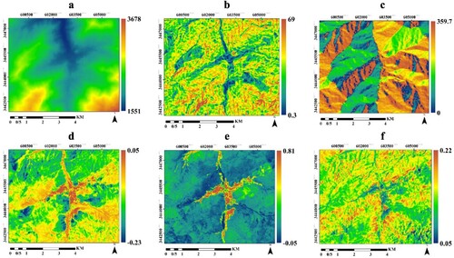
The environmental variables of the region have a heterogeneous spatial distribution (Figure 3).

Figure 3. The maps of the various environmental variables (a) DEM, (b) Slope, (c) Aspect, (d) Wetness, (e) NDVI, and (f) Albedo.

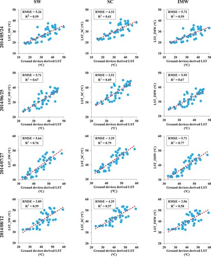
The accuracy of the SC algorithm was higher than that of SW and IMW algorithms on 24/05/2014, 25/06/2014, and 27/07/2014. Except for 12/08/2014, the SW algorithm yielded the best LST calculation accurecy (Figure 4). The main reason for the relatively large difference between the calculated and measured LST is the heterogeneous topographic condition of the region. In this study, the mean value of the determination coefficient was achieved at 0.67. While this value was 0.45 for the LST obtained from AST08 product and ground-based devices in the study by Malbéteau et al. (2017) who had used the same ground devices to retrieve LST in the same location.

Figure 4. The accuracy of LST obtained from different algorithms.

The most accurate LST maps and effective cumulative solar irradiance on different dates are shown in Figure 5. The mean (standard deviation) of satellite image-derived LST values on 24/05/2014, 25/06/2014, 27/07/2014, and 12/08/2014 were 28.8 (5.0), 35.1 (4.6), 41.1 (6.1) and 43.6 (6.2) °C, respectively.

Figure 5. Optimal LST maps (°C) and effective cumulative solar irradiance (W m⁻²).

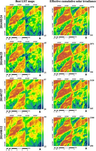
Regarding heterogeneous topographic conditions over the region, different effects of effective cumulative solar irradiance on each point of surface are due to the variations in the local incidence angle of solar rays. Figure 5 shows these large variations. In addition, the heterogeneous distribution of the environmental variables caused large variations in LST in the spatial dimension of the region.

4.2. Sensitivity analysis of impact of environmental variables on LST

The standard deviations of LST corresponding to 24/05/2014, 25/06/2014, 27/07/2014, and 12/08/2014 were 7.22, 6.52, 10.50, and 12.47 °C, respectively. The difference in LST standard deviations on different dates indicates that the environmental variables have different effects on LST given the time. The values of determination coefficients, RMSE, and standard deviation based on environmental variables for several dates derived with PLSR model are shown in Figure 6. The results demonstrated in Figure 6 imply that by adding each environmental variable to the PLSR model, the RMSE value between modeled LST and satellite image-derived LST is decreased, whereas the coefficient of determination is increased. Meanwhile, the normalized LST standard deviation is significantly reduced. Considering a certain number of environmental variables and using a local rather than a global optimization strategy are effective in LST normalization based on PLSR model. Depending on the conditions of the region, different environmental variables have different effects on LST. For all dates, the maximum reduction in the standard deviation of normalized LST values was related to the effective cumulative solar irradiance parameter. Therefore, among the environmental variables, effective cumulative solar irradiance is the most effective in the distribution of the LST values. The coefficient of determination between mean values of satellite image-derived LST and effective cumulative solar irradiance on different dates was 0.87.

Figure 6. RMSE and coefficient of determination between the modeled LST and satellite image-derived LST and standard deviation of the normalized LST with the addition of each environmental variable to the normalization model.

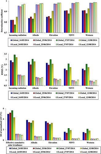
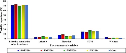
The mean values of the important variables obtained from the RFR model for Effective solar iiradiation, Albedo, Elevation, NDVI, and Wetness respectively were 71.5, 3.75, 7.00, 15.75, and 2.00 in the LST modeling (Figure 7). Among the environmental variables, Incoming radiation and Wetness had the highest and lowest impacts on LST modeling based on RFR model, respectively.

Figure 7. The variable importance of each of the environmental variables in modeling LST.

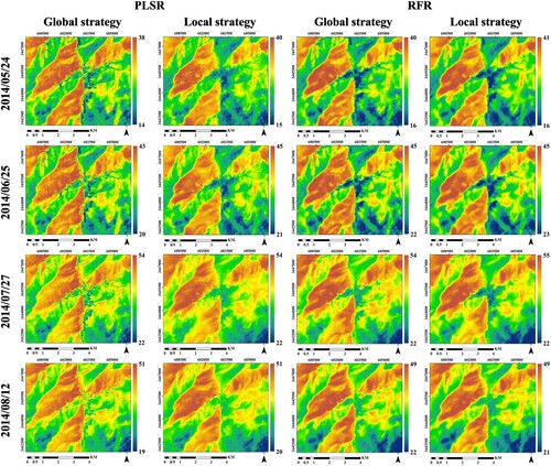
4.3. Modeled and normalized LST

The results of the modeled LST with respect to the environmental variables for various dates are shown in Figure 8. The mean values of the modeled LST obtained from RFR (PLSR) for the global optimization strategy were 28.8 (28.9), 34.3 (34.3), 41.1 (41.2), and 28.2 (37.9) °C on 24/05/2014, 25/06/2014, 27/07/2014 and 12/08/2014, respectively. For the local optimization strategy, these mean values were 28.9 (29.1), 34.4 (34.4), 41.3 (41.5), and 38.4 (38.1) °C, respectively.

Figure 8. The original LST and modeled LST (°C) maps based on PLSR and RFR with global and local optimization strategies.

The RMSE values were lower and the coefficient of determination values were higher in the local optimization strategy than in the global optimization strategy related to PLSR and RFR for all dates (Table 2). The mean values of RMSE and determination coefficient between the satellite image-derived LST and the modeled LST based on PLSR (RFR) were 2.202 °C (0.935 °C) and 0.820 (0.965) for the global optimization strategy and 0.939 °C (0.835 °C) and 0.965 (0.980) for the local optimization strategy, respectively. In addition, RMSE values were lower and coefficient of determination values were higher in RFR compared to PLSR. The significance of the determination coefficient and RMSE values ⁣⁣obtained for the relationship between the satellite imagery-derived LST and modeled LST in all cases have been studied and confirmed at a confidence level of 0.95.

Table 2. The RMSE (Coefficient of determination) between the modeled LST and satellite image-derived LST.

Date	PLSR		RFR
	Global strategy	Local strategy	Global strategy	Local strategy
2014/05/24	2.09 (0.82)	0.96 (0.96)	0.96 (0.96)	0.88 (0.98)
2014/06/25	1.95 (0.83)	0.94 (0.96)	0.94 (0.96)	0.82 (0.97)
2014/07/27	2.54 (0.77)	0.84 (0.97)	0.84 (0.97)+	0.91 (0.98)
2014/08/12	2.23 (0.86)	1.00 (0.97)	1.00 (0.97)	0.73 (0.99)

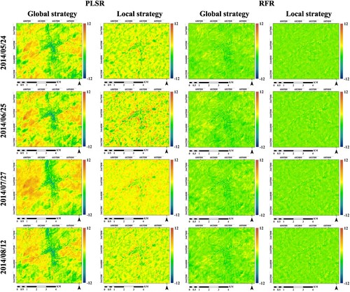
The obtained normalized LST using the modeled LST is presented in Figure 9. Results show that LST has been significantly normalized in terms of environmental variables. After LST normalization for the environmental variables, the heterogeneity of LST distribution was reduced across the study area.

Figure 9. Normalized LST (°C) relative to the environmental variables based on PLSR and RFR with global and local optimization strategies.

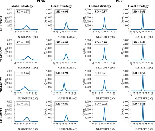
The average standard deviations of the normalized LST based on PLSR (RFR) obtained from the global and local optimization strategies were 2.19 (0.83) and 0.90 (0.50) °C, respectively (Figure 10). The histogram of normalized LST values with the local optimization strategy turned into a narrow bell, which indicates the normal distribution of normalized LST. The normalization performance of the RFR model was higher than that of the PLSR model in both global and local optimization strategies.

Figure 10. The standard deviation and histogram of normalized LST values based on PLSR and RFR with global and local optimization strategies.

In order to examine the performance of the proposed model for LST normalization, the relationship between environmental variables, satellite image-derived LST, and normalized LST of the region was investigated. The results of the determination coefficients are presented in Table 3.

Table 3. Correlation coefficient related to the relationship between environmental variables, satellite image-derived LST, and normalized LST.

		Effective cumulative solar irradiance	Albedo	Elevation	NDVI	Wetness
2014/05/24	Satellite image-derived LST	0.8187	0.1466	−0.1483	−0.4187	−0.2443
	NLSTGPLSR (GRFR)	−0.023 (−0.005)	−0.0531 (0.003)	0.0945 (−0.008)	−0.0172 (0.007)	0.0141 (0.004)
	NLSTLPLSR (LRFR)	0.0148 (0.004)	−0.0020 (−0.001)	0.0051 (−0.005)	−0.0081 (−0.007)	0.0023 (−0.002)
2014/06/25	Satellite image-derived LST	0.8203	0.2078	0.1953	−0.4102	−0.2312
	NLSTGPLSR (GRFR)	−0.0259 (0.006)	−0.0330 (0.005)	0.0678 (−0.003)	−0.0170 (−0.002)	0.0085 (−0.007)
	NLSTLPLSR (LRFR)	0.0206 (−0.003)	0.0075 (−0.004)	−0.0100 (−0.001)	−0.0081 (−0.002)	−0.0066 (−0.004)
2014/07/27	Satellite image-derived LST	0.7754	0.2870	−0.3839	−0.2523	−0.2857
	NLSTGPLSR (GRFR)	−0.0125 (0.007)	−0.0678 (−0.009)	0.1683 (0.011)	−0.0337 (−0.008)	0.0655 (−0.006)
	NLSTLPLSR (LRFR)	0.0074 (0.004)	0.0213 (−0.006)	−0.0181 (0.004)	−0.0246 (−0.006)	−0.0214 (−0.005)
2014/08/12	Satellite image-derived LST	0.8493	0.2352	−0.4825	−0.1730	−0.2125
	NLSTGPLSR (GRFR)	−0.0246 (0.005)	−0.0390 (−0.012)	0.0694 (−0.008)	−0.0278 (−0.006)	−0.0390 (−0.007)
	NLSTLPLSR (LRFR)	0.0102 (−0.002)	0.0138 (0.006)	−0.0243 (−0.005)	−0.0054 (−0.003)	−0.0148 (−0.004)

The correlation coefficient is close to 0 for the relationship between the normalized LST and all the given environmental variables (Table 3). Therefore, normalized LST is independent of all variables considered in this study. The significance of the correlation coefficient values ⁣⁣for the relationships between each variable with satellite image-derived LST and normalized LST were studied and confirmed at a confidence level of 0.95. Table 3 shows the performance results of the proposed model for LST normalization relative to the environmental variables. The local optimization strategy was more efficient than the global optimization strategy in LST normalization. Moreover, the RFR model outperformed the PLSR model in LST normalization. For all dates, the determination coefficient between the effective cumulative solar irradiance and LST was the highest, which indicates the high effect of this parameter on the satellite image-derived LST in the region. Regarding field information and lack of geothermal resources in the study area, it can be concluded that the remaining thermal anomalies concerning normalized LST were related to other environmental variables such as thermal inertia.

4.4. Assessment of the models’ performance based on the ground-device derived LST

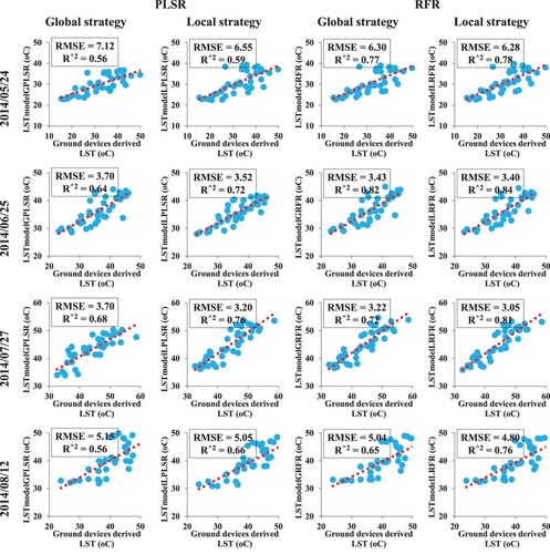
The mean values of RMSE and the coefficient of determination between the measured soil temperatures and modeled LST based on PLSR (RFR) were 4.91 °C (4.50 °C) and 0.61 (0.74) in the global optimization strategy, while these values were 4.58 °C (4.38 °C) and 0.68 (0.79) in the local optimization strategy (Figure 11). In all four Landsat 8 images, the values ⁣⁣of RMSE between ground device-derived LST and modeled LST showed that the local optimization strategy was more efficient than the global optimization strategy at normalizing LST. The RFR model also outperformed PLSR in normalizing LST. The mean value of the coefficients of determination between soil temperatures measured by ground-based devices and obtained from satellite images was obtained at 0.47 in the study by Malbéteau et al. (2017).

Figure 11. The RMSE (°C) and coefficient of determination between modeled LST and ground device-derived LST.

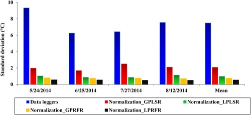
The mean standard deviation of soil temperatures measured by ground-based devices for various dates was obtained at 7.48 °C² (Figure 12). The high value of this factor indicates that the devices were placed in locations with highly heterogeneous environmental characteristics. The standard deviation was significantly decreased after LST normalization. The standard deviation of normalized LST values in the geographic location of the ground devices was lower in the local than the global optimization as well as in the RFR than the PLSR model for all dates.

Figure 12. The standard deviation of ground device-derived LST and normalized LST in location of ground devices.

5. Discussion

Normalization of LST relative to environment variables is very important in many environmental applications. The review results revealed that the proposed models for LST normalization have emphasized the effective role of solar and topographic conditions. Most of the proposed models are suitable for dry areas (Coolbaugh et al. 2007). Various studies in this field, except for Coolbaugh et al. (2007), have considered the effect of instantaneous solar irradiance on LST. This is while the recorded surface temperature was continuous in the radiation region from sunrise to the satellite overpass. Hence, this study considered the effect of effective cumulative solar irradiance in the LST normalization process. Moreover, in the proposed model, the environmental variables related to the SEB components such as net radiation, latent, and sensible heat fluxes including effective cumulative solar irradiance, NDVI, DEM, and wetness were factored in for LST normalization. However, in previous studies, many of these variables including vegetation and surface wetness were not accounted for LST normalization in various applications such as the identification of geothermal regions (Coolbaugh et al. 2007; Gutiérrez et al. 2012).

On the other hand, the use of the OLS model could be associated with some fundamental challenges such as sensitivity to the correlation among environmental variables, the small number of samples, the initial assumption of normal distribution of input data, and the lack of data outliers. One of the strengths of the present study is the use of PLSR and RFR models with global and local optimization strategies for solving the regression coefficients of the normalization. Compared to OLS, these models have a lower sensitivity to the correlation between the environmental variables, the distribution model of variables, and the number of parameter values (Farifteh et al. 2007; de Paulo, Barros, and Barbeira 2016). The accuracy assessment results are indicative of significantly improved LST normalization results compared to those obtained from the study by Malbéteau et al. (2017). It should be noted that compared to OLSR, the use of PLSR and RFR for optimizing the regression coefficients in the LST normalization model yielded more accurate results. One of the limitations in the use of RFR is that it is a black-box algorithm. However, this model has a high ability to accurately construct a nonlinear model between LST and a set of environmental variables (Hutengs and Vohland 2016; Sismanidis et al. 2017; Yang et al. 2017; Zhao et al. 2019).

Most of the previous studies have used a multi-linear regression model and tried to find the regression coefficients by a global optimization method (Verhoest et al. 2012; Malbéteau et al. 2017; Zhao et al. 2019). To improve the LST normalization results, the regression coefficients of different models for each pixel could be calculated by a local optimization method based on the values of neighboring pixels (Weng et al. 2019). Another strength of the present study is the use of a local optimization strategy for LST normalization. Results showed that a local optimization strategy has a significantly higher efficiency than global optimization in this regard (Table 2; Figures 10–12).

The remaining surface temperature in normalized LST was considered a thermal anomaly (Figure 9). The variety of the remaining temperature values in normalized LST can be due to different reasons. First, the effects of the considered variables have not been well modeled in the proposed model and so were not removed from the LST. Second, this region’s LST is under the influence of other variables such as thermal inertia, human activities, and solar irradiance related to the previous day, which were not considered in the proposed model. Third, this region is also affected by geothermal resources.

6. Conclusion

For various scientific and application-based studies, the LST modeling and normalization is very important. The purpose of this research is to present models based on PLSR and RFR with two global and local strategies to normalize LST. According to the sensitivity analysis, the environmental factor of effective cumulative solar irradiance is the most influential factor in the spatial distribution of LST in daytime. The results indicated that effective cumulative solar irradiance was the most effective parameter on the spatial distribution of LST. The relationship between the environmental variables and LST before and after normalization confirms the efficiency of the proposed model for normalizing LST. The determination coefficient of the relationship between the environmental variables and LST after normalization shows a numerical value very close to zero. For the global optimization strategy using PLSR (RFR), the determination coefficient and RMSE values were, respectively, obtained at 0.820 (0.965) and 2.202 °C (0.935°C) between modeled LST and satellite imagery-derived LST and 0.61 (0.74) and 4.91 °C (4.50°C) between modeled LST and ground device-derived LST. For the local optimization strategy, these values were measured at 0.965 (0.980), 0.939 °C (0.835°C), 0.68 (0.79), and 4.58 °C (4.38°C), respectively. The normalized LST standard deviations obtained from the PLSR (RFR) for global and local optimization strategies were 2.19 (0.83) and 0.90 (0.50) °C, respectively. For LST normalization, the local optimization strategy has a significantly higher efficiency than global optimization. Moreover, the RFR model has a higher performance than PLSR in terms of LST normalization. In future studies, it is suggested to consider the effect of other environmental variables affecting LST including thermal inertia as well as barometric elevation using night-time thermal imagery for the normalization model.

Data availability statement

The data that support the findings of this study are available from the corresponding author upon reasonable request.

Disclosure statement

No potential conflict of interest was reported by the author(s).

References

- Alavipanah, S. K., M. Kiavarz, and M. K. Firozjaei. 2017. “Monitoring Spatiotemporal Changes of Heat Island in Babol City due to Land use Changes. International Archives of the Photogrammetry.” Remote Sensing & Spatial Information Sciences 42: 1–11.
- Allen, R. G., R. Trezza, and M. Tasumi. 2006. “Analytical Integrated Functions for Daily Solar Radiation on Slopes.” Agricultural and Forest Meteorology 139 (1): 55–73.
- Amiri, R., Q. Weng, A. Alimohammadi, and S. K. Alavipanah. 2009. “Spatial–Temporal Dynamics of Land Surface Temperature in Relation to Fractional Vegetation Cover and Land Use/Cover in the Tabriz Urban Area, Iran.” Remote Sensing of Environment 113 (12): 2606–2617.
- Anderson, M. C., R. G. Allen, A. Morse, and W. P. Kustas. 2012. “Use of Landsat Thermal Imagery in Monitoring Evapotranspiration and Managing Water Resources.” Remote Sensing of Environment 122: 50–65.
- Barsi, J. A., J. R. Schott, S. J. Hook, N. G. Raqueno, B. L. Markham, and R. G. Radocinski. 2014. “Landsat-8 Thermal Infrared Sensor (TIRS) Vicarious Radiometric Calibration.” Remote Sensing 6 (11): 11607–11626.
- Berger, C., J. Rosentreter, M. Voltersen, C. Baumgart, C. Schmullius, and S. Hese. 2017. “Spatio-Temporal Analysis of the Relationship Between 2D/3D Urban Site Characteristics and Land Surface Temperature.” Remote Sensing of Environment 193: 225–243.
- Boudhar, A., B. Duchemin, L. Hanich, G. Boulet, and A. Chehbouni. 2011. “Spatial Distribution of the Air Temperature in Mountainous Areas Using Satellite Thermal Infra-red Data.” Comptes Rendus Geoscience 343 (1): 32–42.
- Breiman, L. 2001. “Random Forests.” Machine Learning 45 (1): 5–32.
- Coolbaugh, M., C. Kratt, A. Fallacaro, W. Calvin, and J. Taranik. 2007. “Detection of Geothermal Anomalies Using Advanced Spaceborne Thermal Emission and Reflection Radiometer (ASTER) Thermal Infrared Images at Bradys Hot Springs, Nevada, USA.” Remote Sensing of Environment 106 (3): 350–359.
- Danielson, E. W., J. Levin, and E. Abrams. 2003. Meteorology. Columbus: McGraw-Hill.
- de Paulo, J. M., J. E. Barros, and P. J. Barbeira. 2016. “A PLS Regression Model Using Flame Spectroscopy Emission for Determination of Octane Numbers in Gasoline.” Fuel 176: 216–221.
- Farifteh, J., F. Van der Meer, C. Atzberger, and E. Carranza. 2007. “Quantitative Analysis of Salt-Affected Soil Reflectance Spectra: A Comparison of Two Adaptive Methods (PLSR and ANN).” Remote Sensing of Environment 110 (1): 59–78.
- Firozjaei, M. K., S. Fathololoumi, S. K. Alavipanah, M. Kiavarz, A. R. Vaezi, and A. Biswas. 2020a. “A New Approach for Modeling Near Surface Temperature Lapse Rate Based on Normalized Land Surface Temperature Data.” Remote Sensing of Environment 242: 111746.
- Firozjaei, M. K., M. Kiavarz, and S. K. Alavipanah. 2022a. “Impact of Surface Characteristics and Their Adjacency Effects on Urban Land Surface Temperature in Different Seasonal Conditions and Latitudes.” Building and Environment 219: 109145.
- Firozjaei, M. K., M. Kiavarz, and S. K. Alavipanah. 2022b. “Quantification of Landscape Metrics Effects on Downscaled Urban Land Surface Temperature Accuracy of Satellite Imagery.” Advances in Space Research 70 (1): 35–47.
- Firozjaei, M. K., M. Kiavarz, S. K. Alavipanah, T. Lakes, and S. Qureshi. 2018. “Monitoring and Forecasting Heat Island Intensity Through Multi-Temporal Image Analysis and Cellular Automata-Markov Chain Modelling: A Case of Babol City, Iran.” Ecological Indicators 91: 155–170.
- Firozjaei, M. K., Q. Weng, C. Zhao, M. Kiavarz, L. Lu, and S. K. Alavipanah. 2020b. “Surface Anthropogenic Heat Islands in Six Megacities: An Assessment Based on a Triple-Source Surface Energy Balance Model.” Remote Sensing of Environment 242: 111751.
- Friedl, M. 2002. “Forward and Inverse Modeling of Land Surface Energy Balance Using Surface Temperature Measurements.” Remote Sensing of Environment 79 (2): 344–354.
- Giridharan, R., and R. Emmanuel. 2018. “The Impact of Urban Compactness, Comfort Strategies and Energy Consumption on Tropical Urban Heat Island Intensity: A Review.” Sustainable Cities and Society 40: 677–687.
- Gutiérrez, F. J., M. Lemus, M. A. Parada, O. M. Benavente, and F. A. Aguilera. 2012. “Contribution of Ground Surface Altitude Difference to Thermal Anomaly Detection Using Satellite Images: Application to Volcanic/Geothermal Complexes in the Andes of Central Chile.” Journal of Volcanology and Geothermal Research 237-238: 69–80.
- Han, Y., Y. Wang, and Y. Zhao. 2010. “Estimating Soil Moisture Conditions of the Greater Changbai Mountains by Land Surface Temperature and NDVI.” IEEE Transactions on Geoscience and Remote Sensing 48 (6): 2509–2515.
- Hantson, S., and E. Chuvieco. 2011. “Evaluation of Different Topographic Correction Methods for Landsat Imagery.” International Journal of Applied Earth Observation and Geoinformation 13 (5): 691–700.
- Harris, P. P., S. S. Folwell, B. Gallego-Elvira, J. Rodríguez, S. Milton, and C. M. Taylor. 2017. “An Evaluation of Modeled Evaporation Regimes in Europe Using Observed dry Spell Land Surface Temperature.” Journal of Hydrometeorology 18 (5): 1453–1470.
- Hassan, Q., C. Bourque, F.-R. Meng, and R. Cox. 2007. “A Wetness Index Using Terrain-Corrected Surface Temperature and Normalized Difference Vegetation Index Derived from Standard MODIS Products: An Evaluation of Its Use in a Humid Forest-Dominated Region of Eastern Canada.” Sensors 7 (10): 2028–2048.
- He, J., W. Zhao, A. Li, F. Wen, and D. Yu. 2018. “The Impact of the Terrain Effect on Land Surface Temperature Variation Based on Landsat-8 Observations in Mountainous Areas.” International Journal of Remote Sensing 40: 1–20.
- Hongchao, M., and L. Deren. 2001. “Enhancing Group Resolution of TM6 Based on Multi-Variate Regression Model and Semi-Variogram Function.” Geo-spatial Information Science 4 (1): 43–49.
- Hutengs, C., and M. Vohland. 2016. “Downscaling Land Surface Temperatures at Regional Scales with Random Forest Regression.” Remote Sensing of Environment 178: 127–141.
- Jacobson, M. Z. 2005. Fundamentals of Atmospheric Modeling. Cambridge: Cambridge University Press.
- Jia, L., M. Marco, S. Bob, J. Lu, and M. Massimo. 2017. “Monitoring Water Resources and Water Use from Earth Observation in the Belt and Road Countries.” Bulletin of Chinese Academy of Sciences 32 (Z1): 62–73.
- Jimenez-Munoz, J. C., J. A. Sobrino, D. Skokovic, C. Mattar, and J. Cristobal. 2014. “Land Surface Temperature Retrieval Methods from Landsat-8 Thermal Infrared Sensor Data.” IEEE Geoscience and Remote Sensing Letters 11 (10): 1840–1843. English.
- Jiménez-Muñoz, J. C., J. A. Sobrino, D. Skoković, C. Mattar, and J. Cristóbal. 2014. “Land Surface Temperature Retrieval Methods from Landsat-8 Thermal Infrared Sensor Data.” IEEE Geoscience and Remote Sensing Letters 11 (10): 1840–1843.
- Kalogirou, S. A. 2013. Solar Energy Engineering: Processes and Systems. Cambridge: Academic Press.
- Karnieli, A., N. Agam, R. T. Pinker, M. Anderson, M. L. Imhoff, G. G. Gutman, N. Panov, and A. Goldberg. 2010. “Use of NDVI and Land Surface Temperature for Drought Assessment: Merits and Limitations.” Journal of Climate 23 (3): 618–633.
- Li, Z.-L., B.-H. Tang, H. Wu, H. Ren, G. Yan, Z. Wan, I. F. Trigo, and J. A. Sobrino. 2013. “Satellite-Derived Land Surface Temperature: Current Status and Perspectives.” Remote Sensing of Environment 131: 14–37.
- Lievens, H., B. Martens, N. Verhoest, S. Hahn, R. Reichle, and D. Miralles. 2017. “Assimilation of Global Radar Backscatter and Radiometer Brightness Temperature Observations to Improve Soil Moisture and Land Evaporation Estimates.” Remote Sensing of Environment 189: 194–210.
- Liu, Q., G. Liu, C. Huang, and C. Xie. 2015. “Comparison of Tasselled Cap Transformations Based on the Selective Bands of Landsat 8 OLI TOA Reflectance Images.” International Journal of Remote Sensing 36 (2): 417–441.
- Ma, J., S. Chen, X. Hu, P. Liu, and L. Liu. 2010. “Spatial-Temporal Variation of the Land Surface Temperature Field and Present-day Tectonic Activity.” Geoscience Frontiers 1 (1): 57–67.
- Malbéteau, Y., O. Merlin, S. Gascoin, J.-P. Gastellu, C. Mattar, L. Olivera-Guerra, S. Khabba, and L. Jarlan. 2017. “Normalizing Land Surface Temperature Data for Elevation and Illumination Effects in Mountainous Areas: A Case Study Using ASTER Data Over a Steep-Sided Valley in Morocco.” Remote Sensing of Environment 189: 25–39.
- Mansor, S., A. Cracknell, B. Shilin, and V. Gornyi. 1994. “Monitoring of Underground Coal Fires Using Thermal Infrared Data.” International Journal of Remote Sensing 15 (8): 1675–1685.
- Mattar, C., B. Franch, J. Sobrino, C. Corbari, J. Jiménez-Muñoz, L. Olivera-Guerra, D. Skokovic, G. Sória, R. Oltra-Carriò, and Y. Julien. 2014. “Impacts of the Broadband Albedo on Actual Evapotranspiration Estimated by S-SEBI Model Over an Agricultural Area.” Remote Sensing of Environment 147: 23–42.
- Merlin, O., and A. Chehbouni. 2004. “Different Approaches in Estimating Heat Flux Using Dual Angle Observations of Radiative Surface Temperature.” International Journal of Remote Sensing 25 (1): 275–289.
- Mijani, N., S. K. Alavipanah, S. Hamzeh, M. K. Firozjaei, and J. J. Arsanjani. 2019. “Modeling Thermal Comfort in Different Condition of Mind Using Satellite Images: An Ordered Weighted Averaging Approach and a Case Study.” Ecological Indicators 104: 1–12.
- Minder, J. R., P. W. Mote, and J. D. Lundquist. 2010. “Surface Temperature Lapse Rates Over Complex Terrain: Lessons from the Cascade Mountains.” Journal of Geophysical Research 115: D14.
- Mousivand, A., W. Verhoef, M. Menenti, and B. Gorte. 2015. “Modeling top of Atmosphere Radiance Over Heterogeneous Non-Lambertian Rugged Terrain.” Remote Sensing 7 (6): 8019–8044.
- Pardo-Igúzquiza, E., M. Chica-Olmo, and P. M. Atkinson. 2006. “Downscaling Cokriging for Image Sharpening.” Remote Sensing of Environment 102 (1-2): 86–98.
- Proy, C., D. Tanre, and P. Deschamps. 1989. “Evaluation of Topographic Effects in Remotely Sensed Data.” Remote Sensing of Environment 30 (1): 21–32.
- Rodriguez-Galiano, V., E. Pardo-Igúzquiza, M. Sanchez-Castillo, M. Chica-Olmo, and M. Chica-Rivas. 2012. “Downscaling Landsat 7 ETM+ Thermal Imagery Using Land Surface Temperature and NDVI Images.” International Journal of Applied Earth Observation and Geoinformation 18: 515–527.
- Rolland, C. 2003. “Spatial and Seasonal Variations of air Temperature Lapse Rates in Alpine Regions.” Journal of Climate 16 (7): 1032–1046.
- Silva, B. B. D., A. C. Braga, C. C. Braga, L. M. de Oliveira, S. M. Montenegro, and B. Barbosa Junior. 2016. “Procedures for Calculation of the Albedo with OLI-Landsat 8 Images: Application to the Brazilian Semi-Arid.” Revista Brasileira de Engenharia Agrícola e Ambiental 20 (1): 3–8.
- Sismanidis, P., I. Keramitsoglou, B. Bechtel, and C. Kiranoudis. 2017. “Improving the Downscaling of Diurnal Land Surface Temperatures Using the Annual Cycle Parameters as Disaggregation Kernels.” Remote Sensing 9 (1): 23.
- Tachikawa, T., M. Kaku, A. Iwasaki, D. B. Gesch, M. J. Oimoen, Z. Zhang, J. J. Danielson, T. Krieger, B. Curtis, and J. Haase. 2011. ASTER Global Digital Elevation Model Version 2-Summary of Validation Results. Washington, D.C.: NASA.
- Tucker, C. J. 1979. “Red and Photographic Infrared Linear Combinations for Monitoring Vegetation.” Remote Sensing of Environment 8 (2): 127–150.
- Verhoest, N. E., J. Peters, B. De Baets, E. M. De Clercq, and E. Ducheyne. 2012. “Influence of Topographic Normalization on the Vegetation Index-Surface Temperature Relationship.” Journal of Applied Remote Sensing 6 (1): 063518.
- Vlassova, L., F. Pérez-Cabello, M. R. Mimbrero, R. M. Llovería, and A. García-Martín. 2014. “Analysis of the Relationship Between Land Surface Temperature and Wildfire Severity in a Series of Landsat Images.” Remote Sensing 6 (7): 6136–6162.
- Voogt, J. A., and T. R. Oke. 2003. “Thermal Remote Sensing of Urban Climates.” Remote Sensing of Environment 86 (3): 370–384.
- Wang, F., Z. Qin, C. Song, L. Tu, A. Karnieli, and S. Zhao. 2015. “An Improved Mono-Window Algorithm for Land Surface Temperature Retrieval from Landsat 8 Thermal Infrared Sensor Data.” Remote Sensing 7 (4): 4268–4289.
- Weng, Q., M. K. Firozjaei, M. Kiavarz, S. K. Alavipanah, and S. Hamzeh. 2019. “Normalizing Land Surface Temperature for Environmental Parameters in Mountainous and Urban Areas of a Cold Semi-Arid Climate.” Science of The Total Environment 650: 515–529.
- Yang, Y., C. Cao, X. Pan, X. Li, and X. Zhu. 2017a. “Downscaling Land Surface Temperature in an Arid Area by Using Multiple Remote Sensing Indices with Random Forest Regression.” Remote Sensing 9 (8): 789.
- Yang, Y., X. Li, X. Pan, Y. Zhang, and C. Cao. 2017b. “Downscaling Land Surface Temperature in Complex Regions by Using Multiple Scale Factors with Adaptive Thresholds.” Sensors 17 (4): 744.
- Yu, X., X. Guo, and Z. Wu. 2014. “Land Surface Temperature Retrieval from Landsat 8 TIRS—Comparison Between Radiative Transfer Equation-Based Method, Split Window Algorithm and Single Channel Method.” Remote Sensing 6 (10): 9829–9852.
- Zhan, W., Y. Chen, J. Wang, J. Zhou, J. Quan, W. Liu, and J. Li. 2012. “Downscaling Land Surface Temperatures with Multi-Spectral and Multi-Resolution Images.” Int J Appl Earth Obs 18: 23–36.
- Zhang, Y., I. O. Odeh, and C. Han. 2009. “Bi-Temporal Characterization of Land Surface Temperature in Relation to Impervious Surface Area, NDVI and NDBI, Using a Sub-Pixel Image Analysis.” Int J Appl Earth Obs 11 (4): 256–264.
- Zhao, W., S.-B. Duan, A. Li, and G. Yin. 2019. “A Practical Method for Reducing Terrain Effect on Land Surface Temperature Using Random Forest Regression.” Remote Sensing of Environment 221: 635–649.
- Zhao, W., H. Wu, G. Yin, and S.-B. Duan. 2019. “Normalization of the Temporal Effect on the MODIS Land Surface Temperature Product Using Random Forest Regression.” ISPRS Journal of Photogrammetry and Remote Sensing 152: 109–118.