Wind resistance aerial path planning for efficient reconstruction of offshore ship

ABSTRACT

When the unmanned aerial vehicle (UAV) is applied to three-dimensional (3D) reconstruction of the offshore ship, it faces two problems: the battery capacity limitation of the UAV and the disturbance of the wind in the environment. Wind disturbance is generally not considered in the path planning process of the existing UAV 3D reconstruction path planning research. Therefore, the planned path is only suitable for no-wind or light-wind scenarios. For the 3D reconstruction of ship targets, we propose a UAV path planning method that can satisfy both reconstruction efficiency and wind disturbance resistance requirements. Firstly, the concept of model surface complexity is proposed to generate a more efficient candidate view set. Secondly, the Min–Max strategy and a new viewpoint construction method are used to generate the initial path. Thirdly, combined with the wind field model, a method for generating a stable path against wind disturbance based on the idea of interval optimization is proposed. Experimental results demonstrate that our method can adaptively determine the number of sample points and viewpoints according to ship’s geometric characteristics and further reduce the number of viewpoints without significantly affecting the reconstruction quality; the path planned by our method is also stable against wind disturbance.

KEYWORDS:

• Multi-view 3D reconstruction
• aerial path planning
• wind resistance
• UAV

1. Introduction

With the development of maritime supervision methods, traditional methods (patrol ships, Vessel Traffic System, etc.) are gradually replaced by the use of UAV. There are lots of advantages of UAV, such as simple operation, low cost, quick response, and wide working range. The application of UAV has been extended to all walks of life, including geographic mapping, agricultural plant protection, rescue and disaster relief, aerial photography. With the development of image-based 3D reconstruction and the commercial UAVs’ imaging systems, UAVs can be used to take aerial photography in complex urban scenes, and then high-quality 3D reconstruction can be achieved through the advanced structure from motion (SFM) (Arce et al. 2020; Schonberger and Frahm 2016; Wu 2013) or multi-view stereo (MVS) (Furukawa and Hernández 2015; Vogiatzis and Hernández 2011). Due to the simple and flexible operation of UAVs and low maintenance costs, efficient and high-quality reconstruction of large-scale urban scenes has become a hot research topic (Drešček et al. 2020; Li et al. 2016; Xu et al. 2016; Yang et al. 2022; Zheng, Wang, and Li 2018). The 3D models reconstructed from aerial images of UAVs can be used for 3D applications such as digital twin, virtual reality (VR), augmented reality (AR), and so on.

The high-precision reconstruction of large-scale urban scenes plays an important role in promoting the development of smart cities (Danilina, Slepnev, and Chebotarev 2018). The study of maritime ship reconstruction helps to promote the development of the smart maritime system. Generally, the UAV has a certain degree of wind resistance ability. However, in consideration of the ever-changing marine meteorological environment, the UAV may not be able to fully with-stand the complex marine environment, resulting in the failure of aerial photography mission. At present, most state-of-the-art methods are based on the white-box test to solve the specific impact of wind disturbance on UAV and design the control algorithm to compensate for the wind disturbance (Dai et al. 2020; Wang et al. 2021; Zhang et al. 2020). However, this kind of wind resistance method is relatively complex. There are many parameters to be adjusted, and the requirements for sensors are relatively high. Considering the limited power of UAVs, most reconstruction methods regard efficient scene acquisition and high-quality reconstruction as the first two goals. Among them, the method of establishing a rough proxy model to design the UAV path is proved to be a good solution (Wu 2013). Zhou et al. (2020) built the geometric proxy model of city scenes by detecting shadow lengths in satellite images. Their method avoids the initial flight and realizes the offline UAV path planning. However, the path generated by this method lacks transition viewpoints between the surfaces of the geometric proxy and does not take into account the situations encountered by offshore ship reconstruction. Although UAV path planning technology has made great progress at present, UAV path planning for offshore ship reconstruction still faces many problems to be solved.

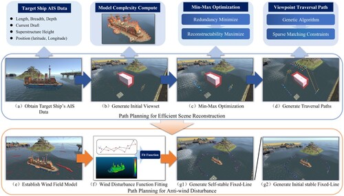
In this paper, we assume that the ship is static and the ship is in any relatively open water or there is no shelter around it. As shown in Figure 1, we propose a UAV path planning method that takes into account both the image acquisition efficiency and the wind disturbance. Firstly, a rough geometric proxy model is generated according to the Automatic Identification System (AIS) data of the ship target, and then the initial view set will be adaptively generated according to the surface complexity of the ship target (Section 3.1). Secondly, according to the heuristic algorithm proposed by Smith et al. (2018), the reconstruction quality of each view pair for sample points is evaluated, and the Min–Max strategy proposed by Zhou et al. (2020) is used to optimize the view set (Section 3.2). Thirdly, based on the optimized sparse matching principle, transition viewpoints between adjacent proxy surfaces are generated, and genetic algorithm is used to solve the traversal path of all viewpoints (Section 3.3). Fourthly, we fit a function between UAV position and attitude offsets and the reconstruction quality based on the system dynamics model of UAV (Section 4.1). Finally, we obtain the wind resistance path based on the interval optimization and fit function (Section 4.2).

Figure 1. The framework of the efficient reconstruction and wind resistance aerial path planning.

The main contributions of our work are summarized as follows:

1. We propose a UAV path planning method for the efficient reconstruction of offshore ship, which takes into account both the reconstruction efficiency and the wind disturbance and solves the wind disturbance problem in marine applications;

2. We introduce the concept of surface complexity, design a surface complexity calculation method for different ship types and take it as the basis for efficient adaptive sampling and view redundancy reduction;

3. We build a virtual scene to validate our UAV path planning method. The system can display the outputs of each step of our algorithm.

2. Related work

2.1. Application of UAV in the field of maritime supervision

Based on the imaging system of UAVs, UAVs are widely used in maritime supervision. Li et al. (2021) proposed a ship speed inversion algorithm based on ship wake characteristics. Shen et al. (2020) developed a path planning model for the collaborative detection of ship air pollution by multiple UAVs in a dynamic environment and improved the particle swarm optimization (PSO) algorithm for solving the dynamic path planning model. Yuan et al. (2020) proposed an enhanced tracking algorithm for UAV, which integrated global prediction with gradient detection through a probabilistic framework and ultimately generated a reliable path to guide UAVs to illegal vessels. Zhou, Pan, and Jiang (2019) proposed an improved visual background extractor (ViBe) algorithm to extract the ship target image from the video captured by UAVs and used the monocular target-positioning algorithm to calculate the ship’s spatial position. Their method is used to verify the authenticity and accuracy of AIS data of ship targets.

There are various applications of UAVs in the field of maritime supervision. The purpose of this paper is to design an efficient path for the UAV to obtain a high-quality reconstruction model of the ship target based on multi-view 3D reconstruction. This will achieve an accurate estimation of the height, width, and attitude of the offshore ship. The estimation information can help to judge whether the ship can pass the navigation lock or the bridge, and whether the ship can maintain the stability. Moreover, when a ship collision accident occurs, the accident scene can be reconstructed by our proposed method. This will promote the efficiency of the decision-making during subsequent rescue activities.

2.2. UAV path planning for efficient scene reconstruction

At present, some mature commercial UAV path planning software has appeared in the market, such as DJI-Pilot, DJI-Terria, PIX4D. However, this software can only generate oblique photography routes at fixed heights. Due to the lack of priori information of the scene, it is impossible to evaluate the quality of the generated viewpoint set, which may lead to ‘undersampling’ or ‘oversampling’. The selection of viewpoints is a research hotspot. Although a sufficient number of views are required for scene reconstruction, too many views will not only prolong the processing time, but also introduce noise into the reconstruction process due to the difference of perspective and scale between views, resulting in the decline of final reconstruction quality.

The view selection problem is to calculate the optimal layout of viewpoints, which is also the path planning problem of UAV. A lot of work has been carried out on this problem, which can be mainly divided into two categories according to the presence or absence of scene priori information.

2.2.1. UAV path planning method without scene geometry priori information

The first category is the method without scene geometry priori information. Most methods rely on Next Best View (NBV) or Simultaneous Localization and Mapping (SLAM) technology to realize real-time autonomous exploration of UAVs. Hardouin et al. (2021) proposed a novel NBV path planning algorithm suitable for online surface reconstruction of large-scale scenes with multiple UAVs and a cluster-based 3D reconstruction gain and finally verified the effectiveness of the method in real scenes. Arce et al. (2020) introduced an unsupervised machine learning algorithm into UAV path planning and realized the automatic UAV flight path planning. Huang et al. (2018) proposed an automatic method for image capture. The core of their method is to implement a fast MVS algorithm through a linear iterative method, which makes the online model reconstruction possible. Suzuki et al. (2011) proposed a monocular camera-based UAV SLAM algorithm based on Scale Invariant Feature Transform (SIFT) triangulation features extracted from captured images. Hermann, Ruf, and Weinmann (2021) proposed a three-stage processing method for 3D model construction. First, SLAM algorithm was used to estimate the rough camera trajectory; then MVS was used to estimate the depth of the local images; and finally, the depth was integrated into the global surfel-based model. Kuang et al. (2020) proposed a real-time path planning method for the automatic reconstruction of urban scenes based on UAV. The initial path was generated based on top views, and then the SLAM framework was used to refine the path to capture architectural details.

In addition to using NBV and SLAM methods for autonomous UAV exploration of unknown scenes, Hepp, Nießner, and Hilliges (2018) designed a hierarchical volume representation to distinguish unknown space, free space, and occupied space in the scene and then conducted the UAV path planning based on the information gain formula. Schmid et al. (2020) proposed an online path-planning algorithm based on Rapidly-exploring Random Trees (RRT), a 3D reconstruction gain and the cost-utility formula based on Truncated Signed Distance Field (TSDF). Liu et al. (2021b) proposed a real-time exploration and reconstruction path planning algorithm for the online path planning of scene exploration and building observation by dynamically estimating the 3D bounding boxes of buildings.

2.2.2. UAV path planning method based on scene geometry priori information

The second category is the method based on the priori information of the scene geometry, which is usually implemented through the two-stage UAV flight strategy. The first stage is the exploration stage, in which the UAV only performs a sparse scan to generate a rough scene geometry proxy. The second stage is the design stage, in which the flight path is designed and optimized through the scene geometry proxy model. At present, UAV path planning based on scene geometry proxy has been proved to be an effective reconstruction scheme. Jing et al. (2016) used 2D map data and height information to generate a rough 3D model of the target building and proposed a neighbourhood greedy search algorithm to solve the set coverage problem (SCP) and obtain the most suitable viewpoint set for the reconstruction task. Smith et al. (2018) developed a novel continuous optimization method for UAV aerial images, using a heuristic method to determine the position and direction of viewpoints, so as to improve the quality of multi-view stereo reconstruction. Based on the work of Smith et al. (2018), Zhou et al. (2020) proposed the view redundancy minimization method, which used Min–Max strategy to optimize the initial view set and achieve better reconstruction quality with fewer images. Koch, Körner, and Fraundorfer (2019) proposed a path planning pipeline for UAV 3D reconstruction based on semantic properties. The target object was extracted in the first flight, and then the path planning was described as a discrete view optimization problem to obtain the final optimized path. Zhang et al. (2021) proposed a UAV trajectory planning algorithm based on an RRT framework, which effectively increased the efficiency of image acquisition by combining path planning with view sampling. Yan et al. (2021) proposed a novel path planning method for high-quality reconstruction. By defining the principles of geometric proxy completeness and accuracy, viewpoints with position and orientation constraints were generated and evaluated. Finally, the planned path can be obtained by smoothly connecting the viewpoints.

Different from the existing two-stage methods, our method does not need the first flight. Based on the AIS data of the ship target (ship length, ship breadth, moulded depth, superstructure height, draft, ship position, etc.), we can easily construct a rough ship geometry proxy. Then, we will calculate the reconstruction ability of the initial candidate view set for the scene. We use the Min–Max strategy to optimize the initial view set and introduce transition viewpoints between adjacent surfaces of the proxy to make the method suitable for monomer reconstruction. In addition, considering the geometry differences between different ship types, we introduce the surface complexity definition to measure the complexity of different proxy surfaces and set the sample radius of each proxy surface and the reconstruction threshold in the calculation of view redundancy minimization to further optimize the view set. We will elaborate our work in Section 3.

2.3. Wind resistance and stability of UAV

In maritime applications, UAVs may often perform aerial photography tasks in windy weather conditions. Although UAVs have a certain wind resistance capability, the wind on water is generally stronger than the wind on land. Wind resistance is unavoidable for effective control of UAV on water. At present, there has been a lot of research on UAV wind-resistance technology. Zhang et al. (2016) proposed a 3D fuzzy Proportion Integration Differentiation (PID) control method for attitude control and trajectory tracking of UAV, which was verified in turbulent wind field generated based on the Dryden model. Cai et al. (2019) proposed an attitude control and interference suppression scheme for quadrotors. In their quadrotor dynamic model, PID method is used to make the fully-actuated subsystem converge rapidly and Equivalent-Input-Disturbance (EID) method is used to realize non-linear compensation and disturbance control. Wen, Wang, and Li (2020) proposed a nonlinear inversion based on high order sliding mode control method to solve the trajectory control problem of UAVs with uncertainty and environment interference. Guo et al. (2020) proposed an anti-interference controller based on multiple observers for UAVs. Xi et al. (2021) proposed an anti-wind model for quadrotors (considering aerodynamic effect, gyroscopic effect and wind disturbance) and a flight control scheme based on improved extended state observer (IESO). Liu et al. (2021a) proposed an adaptive Radial Basis Function (RBF) neural network based on backstepping control to deal with the external disturbance of UAV.

Unlike the above work, our method focuses on the UAV’s wind resistance path planning problem. First, according to the UAV anti-wind disturbance control model (Zhang 2020), we fit the law between the reconstruction error and the offset of the UAV under the given wind field. Then, we generate the anti-wind disturbance stable path according to the idea of interval optimization. We will elaborate on our work in Section 4.

3. Efficient reconstruction path planning generation

We first introduce the efficient reconstruction method using UAVs with limited flight endurance in this section.

3.1. Initial view set generation

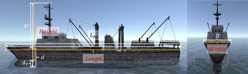
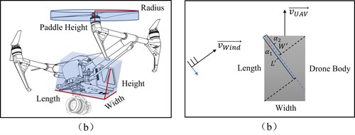
Geometric proxy model construction. According to the international convention for Safety of Life at Sea (SOLAS), all ships of over 300 gross tonnages must be equipped with an AIS, and the AIS should always be kept running. We can easily construct a rough geometric proxy model of the ship based on the ship’s AIS data (length between perpendiculars $l_{bp}$, ship breadth $B$, moulded depth $d$, superstructure height $H$, ship’s current draft $d_r$, ship position). The meaning of each parameter of the ship is shown in Figure 2. Since safe flight is always the primary prerequisite for UAV path planning, we extend the model outward with radius $r$ (adaptive value according to different ship types) to define the no-fly zone of UAV.

Figure 2. Schematic diagram of the length, width and height of the ship geometric proxy model (take the fishing boat as an example).

Model surface complexity calculation. Due to obvious differences in the structure of ships of different types, we propose the concept of model surface complexity to describe the surfaces of the geometric proxy of different ship types. It can guide the setting of the sampling radius and redundancy reduction approach in the subsequent steps.

Definition 3.1:

Minimum included angle: $\theta$.

$\theta$ is the angle that indicates the orientation similarity between the triangular of the ship and the surface of the proxy model. Suppose $\mathrm{M}$ is the mesh model of the specific ship type, $t_{mesh}$ is the triangular surface extracted from $\mathrm{M}$, $\overrightarrow{n_i}$ is the normal vector of each triangular and $\overrightarrow{n_{pi}}$ is the normal vector of each surface of the proxy model (excluding the bottom surface). Then the minimum included angle between $\overrightarrow{n_i}$ and $\overrightarrow{n_{pi}}$ is recorded as $\theta$. (1) $\theta =min\left(\arccos \left({\displaystyle \frac{\overrightarrow{n_i}\cdot \overrightarrow{n_{pi}}}{\left|\overrightarrow{n_i}\right|\left|\overrightarrow{n_{pi}}\right|}}\right)\right)$(1)

Definition 3.2:

Statistical function: $count(\cdot )$.

$count(\cdot )$ is used to count the number of triangles with a similar orientation as the corresponding proxy model surface. Suppose $cnt$ (the initial value is set to 0) is the statistical frequency. If the minimum included angle satisfies $\theta \le {45}^{\circ }$, it is considered that orientation of the triangular is similar to that of the corresponding surface of the geometric proxy model, and $cnt$ will perform an auto-increment operation; if the minimum included angle satisfies $\theta >{45}^{\circ }$, it is considered that orientation of the two surfaces is different, then $cnt$ remains unchanged. Therefore, the statistical function can be designed as following: (2) $count\left(\theta \right)=\{\begin{array}{c}cnt+1,\theta \le {45}^{\circ }\\ cnt,\theta >{45}^{\circ }\end{array}$(2)

Definition 3.3:

Model surface complexity of the proxy model surface: $c_i$.

Assume $s_{pi}$ is the area of the $i$ th proxy model surface, the model surface complexity of the $i$ th proxy model surface is recorded as $c_i$. (3) $c_i={\displaystyle \frac{\sum count\left(\theta \right)}{s_{pi}}}$(3)

The detailed calculation of the model surface complexity is shown in Algorithm 1.

Candidate view set generation. We use Poisson disk sampling to uniformly sample the proxy model surface (except the bottom surface). We set the initial overlap ratio between views of the surface with the highest complexity to 0.85 and calculate the sampling radius. The sampling radii of other surfaces are inversely proportional to the complexity of the corresponding surface. We convert the 2D sampling coordinates obtained by the Poisson disk algorithm into 3D coordinates and finally obtain the sample point set $S=\left\{s_i,n_i\right\}$, where $s_i$ represents the 3D coordinates of the sample points, $n_i$ represents the normal vector of the geometric proxy model surface where the viewpoint is located. We then generate candidate view set according to the method of Zhou et al. (2020). Due to uncertain factors such as wind and waves in the marine scene, if the height of viewpoint is lower than 5 m above the sea level, we will delete it for the sake of flight safety.

3.2. View set optimization based on Min–Max strategy

Calculation of reconstructability and redundancy. In order to evaluate the reconstruction ability of viewpoints, we use the reconstructability heuristic algorithm (Smith et al. 2018) to calculate the reconstruction ability of each view pair and adopt the reconstructability formula proposed in Zhou et al. (2020) to compute the reconstructability of view set for a sample point and adopt the acceleration method to calculate the visibility between the sample point and the viewpoint and the relationship between viewpoints.

Min–Max strategy. We optimize the view set with reference to the Min–Max strategy in Zhou et al. (2020). Different from their method, in which a fixed reconstructability threshold is used to reduce redundancy, our method is based on the surface complexity of the geometric proxy model. First, a fixed value is taken as the reconstructability threshold of the surface with the highest complexity, and the reconstructability threshold of other surfaces is inversely proportional to the surface complexity. Thus, our method can achieve the purpose of reducing redundancy according to surface complexity and further reduces the scale of the view set compared with Zhou et al. (2020).

3.3. Viewpoint traversal path generation

Viewpoint traversal. After optimizing the view set by the previous Min–Max strategy, a minimum view set is obtained to perform the reconstruction. We then need to generate a traversal path that travels through all viewpoints at the lowest flight cost and returns to the starting point, which is a typical Travelling Salesman Problem (TSP). The genetic algorithm is used to solve this problem.

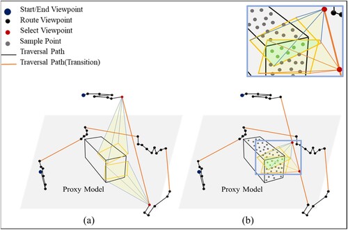
Viewpoint generation on transition path. As shown in Figure 3(a), there is no specific method to generate viewpoints on the path that connects viewpoints of the proxy model surface (the long solid line in Figure 3(a)) in Zhou et al. (2020). This will lead to the lack of necessary image intersection between adjacent proxy model surfaces and eventually lead to failure in the process of multi-view matching.

Figure 3. Schematic diagram of the (a) transition path and (b) transition viewpoint.

Definition 3.4:

Transition path $\xi$.

Assume $v_{fi}$ is the first viewpoint of the proxy model surface $s_i$ and $v_{l_i}$ is the last viewpoint. The transition path segment ${\xi }_i$ is the line segment connecting the last viewpoint $v_{l_i}$ and the first viewpoint $v_{f_i}$ of the adjacent surface. The transition path is the set of all transition path segments, recorded as $\xi$.

Zhou et al. (2020) aim at the reconstruction of buildings in large-scale urban scenes. Their method rotates the blocked viewpoint around the Z axis until the viewpoint meets both the visibility check and collision detection. This method neatly avoids the above problem. However, this is not suitable for the reconstruction of a single ship in the scenes without obstacles.

To address the problem of the lack of sufficient image intersection, we optimize the viewpoint sparse matching constraint (Hepp, Nießner, and Hilliges 2018) to generate viewpoints on the transition path. The transition path will be first sampled uniformly to generate initial sample viewpoints. The sampling radius is set to the average of the sampling radius on the two corresponding proxy model surfaces of the current transition path. The direction of generated viewpoints is oriented towards the centre of the geometric proxy model by default.

Definition 3.5:

Optimized sparse matching constraint (OSMC).

OSMC is an interval that ensures two adjacent viewpoints on the transition path can be matched and the overlap ratio of the two viewpoints is below a threshold. Assume $obs\left(v\right)$ is the function to find the sample points that can be observed by the viewpoint $v$ and $t_{min}$, $t_{max}$ are the lower and upper bounds of the overlap ratio interval, respectively. The optimized sparse matching constraint is described as follows: (4) $t_{\mathrm{m}\mathrm{i}\mathrm{n}}\le {\displaystyle \frac{\left|obs\left(v_1\right)\cap obs\left(v_2\right)\right|}{\left(\left|obs\left(v_1\right)+obs\left(v_2\right)\right|/2\right)}\le t_{\mathrm{m}\mathrm{a}\mathrm{x}}}$(4)

The lower bound $t_{\mathrm{m}\mathrm{i}\mathrm{n}}$ is used to ensure that the two views meet the minimum requirements of multi-view stereo matching, and the upper bound $t_{\mathrm{m}\mathrm{a}\mathrm{x}}$ is used to ensure that the two views will not completely overlap to avoid view redundancy. Our approach is designed to preserve necessary and critical viewpoints on the transition path. After extensive testing, $t_{\mathrm{m}\mathrm{i}\mathrm{n}}=0.4$ and $t_{\mathrm{m}\mathrm{a}\mathrm{x}}=0.8$ can best balance the requirements of stereo matching and redundancy reduction. The detailed calculation of the screening method for sample viewpoints on the transition path is shown in Algorithm 2.

4. Wind resistance path generation

In Section 3, we make important improvements based on the work proposed by Hepp, Nießner, and Hilliges (2018), Smith et al. (2018) and Zhou et al. (2020), and finally generate the efficient reconstruction path of UAVs. Next, we will introduce the generation method of wind resistance path in this section.

Definition 4.1:

Wind resistance path (WRP).

WRP is an optimized path that can resist wind disturbance under a given wind situation, that is, even if the position and attitude of the viewpoints on the path are offset to a certain extent, the final reconstruction quality is still within the pre-set range.

4.1. Fit function of UAV offset and reconstruction error

Creation of wind field model. In order to explore the wind resistance path of UAVs, we first establish a wind field in the scene. In order to ensure the authenticity of the generated wind field, we use the output data of the MM5 model (Jin and Miller 2007), convert the data to 3D wind field layer by layer, and map the 3D wind field to the virtual scene in equal proportions. Figure 4 shows the visualization of the wind field model. In order to enhance the visualization performance, only 20% of grid points of the wind field are displayed (the actual distribution of the wind field is much denser). The wind vane on each grid point of the wind field represents the wind direction and wind force. In order to calculate the wind condition of the UAV in the wind field, we retrieve eight grid points of the wind field that are close to the UAV and record the corresponding wind conditions, and then we use distance weighting interpolation to compute the wind condition at the position of UAV.

Figure 4. Schematic diagram of the wind field. (a) Visualization of the wind field model established in the virtual scene; (b) Wind condition at the position of the UAV. Eight dense wind vanes represent the retrieved grid points in the wind field model, and the middle wind vane represents the wind condition at the position of the UAV.

Quantification of the impact of wind disturbance on UAV. In order to further obtain the position and attitude offset of the UAV under the given wind situation, we refer to the UAV control model under wind disturbance (Zhang 2020) to calculate the offset. Solving this model requires many parameters. Through Shi et al. (2017), we can obtain technical parameters of a certain type of UAV under different motion states to solve the model. Specifically, we need to calculate the windward area of the UAV for model solving. As shown in Figure 5(a), we define the windward area of the UAV as two parts: cuboid-like structure of its main body and four cylinders formed by rotating blades. During the flight, the angle between the wind direction and the UAV’s speed vector is constantly changing. Therefore, we first calculate the angle, and then project the wind vector to calculate the windward area of the UAV in the wind field. The specific method is shown in Figure 5(b). Firstly, the dot product $\mathrm{d}\mathrm{o}{\mathrm{t}}_1$ of the unit normal vector of the wind vector and the UAV speed vector (the module length is set as the length of the main body) is calculated; meanwhile, the dot product $\mathrm{d}\mathrm{o}{\mathrm{t}}_2$ of the unit normal vector of the wind vector and the unit normal vector of the UAV speed vector (the module length is set as the width of the main body) is calculated. Secondly, the product of $\left|do{t}_1\right|+\left|do{t}_2\right|$ and fuselage height is taken as the windward area of the UAV’s main body. For the calculation of the windward area of the cylinder formed by the blades, the wind area can be regarded as half of the surface area of the cylinder without the bottom surface.

Figure 5. Schematic diagram of the windward area. (a) Composition of the UAV’s windward area; (b) The calculation of the windward area of the UAV’s main body.

Through the above steps, the windward area of the UAV is obtained. Thus, we get all the parameters required for the UAV control model under wind disturbance in Zhang (2020), and we use the ode45 solver based on Runge–Kutta method to solve the differential equation in the model. At last, we get the position and pose offset of the UAV under the given wind situation. The UAV’s pan-tilt camera has a certain degree of stability, and we find that the compensation ranges of pitch and roll of the pan-tilt camera have already covered the corresponding offset angles output by the control model by querying the specific technical parameters of common commercial UAVs. Therefore, we only need to consider the effect of the yaw direction in our experiment.

Establishment of the fit function. In order to find the relationship between the influence of wind disturbance on UAV and the reconstruction quality, we first quantify the wind disturbance as the attitude offset (one components) and position offset (three components) of UAV and quantify the reconstruction quality as the distance between the reconstructed model and the ground truth model. We discretize the UAV path into separate viewpoints, that is, the number of independent variables in the final fit function is four times the number of viewpoints. Furthermore, in order to simulate the random variation of the natural wind, we add an additional 20% random disturbance to the position and pose offset of the control model output. Therefore, the independent variables of each viewpoint in the fit function are made up of three position coordinates and one attitude coordinate.

For the measurement of reconstruction quality, we first input the view set obtained by new viewpoints into the Context Capture software and get the reconstructed model. Then, we use the iterative closest point (ICP) method in Cloud Compare software to align the reconstructed model with the ground truth. We allow the size of the mesh model to be changed. After the registration is completed, the mean distance between the two models (reconstruction quality) can be obtained. That is, the dependent variable in the final fit function is obtained.

In order to fit the relationship between the UAV offset and the reconstruction quality, we conducted 300 sets of experiments and use the CNN regression model in Matlab to perform the fitting calculation. The fitting result is acceptable: $R^2=0.98$, $RMSE=0.16$, indicating that the fit function can be used for wind resistance path planning in the subsequent steps.

4.2. Generation of wind resistance path

We adopt the idea of interval optimization to solve this problem. It should be noted that the WRP path under wind disturbance is planned based on the efficient reconstruction path generated in Section 3.

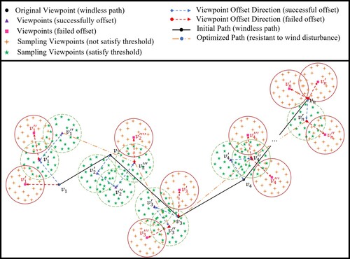
In wind resistance path planning, we optimize each viewpoint on the initial path step by step. The schematic diagram of generating a wind resistance path based on interval optimization is shown in Figure 6, and the specific optimization method is shown in Algorithm 3.

Figure 6. Two-dimensional schematic diagram of the interval optimization process. The circle represents the sampling circle set, and the points in the sampling circle represent the sample viewpoints. The solid sampling circle and the corresponding sample viewpoints indicate that the current viewpoint offset does not meet the generation requirements of the WRP. On the contrary, the dashed ones indicate that the generation requirements of the WRP are met. The dashed path represents the optimized WRP, and the solid path represents the initial windless path.

Definition 4.2:

Initial stable wind resistance path (ISWRP).

ISWRP is the WRP with initial stable performance. Assume $E_i$ is the reconstruction error of the initial path without wind disturbance, and $E_a$ is the mean reconstruction error of the disturbed paths. The ISWRP is supposed to ensure the difference between $E_i$ and $E_a$ is within the allowable threshold.

Definition 4.3:

Self-stable wind resistance path (SWRP).

SWRP is the WRP with self-stable performance. Assume $E_a$ is the variance of the reconstruction error of the disturbed paths. The SWRP is supposed to ensure $E_a$ is within the allowable threshold.

Firstly, we extract the first viewpoint on the initial path, randomly offset its position coordinates and uniformly sample its view direction offset. We record the view direction that can minimize the reconstruction error based on the fit function. This view direction will be set as the final view direction of the viewpoint. Secondly, we take the current viewpoint as the centre of the interval and uniformly sample in the interval with the pre-set sample radius to obtain a set of sample viewpoints and then determine the view direction of the sample viewpoints according to Algorithm 4. Thus, we can calculate the reconstruction error after replacing the current viewpoint with each sample viewpoint.

For different applications, we may need different types of WRP. For ISWRP, we take the distance between the mean reconstruction error of all sample viewpoints and the reconstruction error of the initial path as the threshold to measure whether the current viewpoint should be accepted. For SWRP, we take the variance of reconstruction errors of all sample viewpoints as the threshold to measure whether the current viewpoint should be accepted. The calculation will be repeated until the maximum number of iterations is reached. The process will be repeated for all viewpoints on the path until all viewpoints are optimized.

5. Result and evaluation

5.1. Experiment overview and implementation details

In order to verify the effectiveness and superiority of our method, we compare our method with the work of Zhou et al. (2020) and a well-established oblique photography solution. Our experiments are carried out from three aspects. Firstly, we conducted self-evaluation of our method to test the adaptability of the proxy model, the effectiveness of the two-step strategy, and the effectiveness of ISWRP and SWRP. Secondly, we compare our method with the work of Zhou et al. (2020) and analyse the superiority of our method (significance of introducing model complexity and the necessity of adding transition path). Finally, we compare our method with the well-established oblique photography solution.

Our method is not sensitive to the size of the ship and the battery capacity. Usually, the larger the size of the ship, the more power the UAV will consume. However, the calculation of the specific quantitative relationship needs to comprehensively consider weather conditions (temperature, humidity, wind speed, etc.), UAV model and ship size, which is a complex functional relationship. The UAV can remember the point at which the flight mission was paused and can continue the remaining flight mission at the last paused point. Therefore, the battery capacity of the UAV is not an absolute limiting factor. The purpose of method is to accomplish more tasks with less power. In our method, we do not consider ship size and power consumption as the preconditions of the method. In the simulation experiments, we set the endurance time of the UAV to 25 min and the size of the ship to 140m*20m*25 m. All experiments are tested in a virtual scene built by the Unity 3D platform. The processor of the workstation used to run our method is 2.40 GHz Intel(R) Xeon(R) Silver 4210R, and the graphics card is NVIDIA GeForce RTX 3090. The focal length of the UAV’s pan-tilt camera is 44.7846 mm, the sensor size is 36 mm, and the UAV flies at a constant speed (5 m/s) throughout the whole process. Since we do not reconstruct the bottom surface of the ship, the reconstruction error is relatively large in the following experimental results, which is unavoidable.

5.2. Self-evaluation

Adaptability of the proxy model. The original data used to establish the ship proxy model in our method comes from the AIS information of a ship target. However, the actual draft of the ship in AIS information is sometimes unreliable. In order to verify the adaptability of our method under the condition of an inaccurate proxy model, we artificially impose different degrees of disturbance on the height of the cuboid proxy model.

We use three types of disturbance (10%, 20%, 30%) based on the true height (see Table 1) of the ship target. The quantitative evaluation of the reconstruction error of different disturbances is shown in Table 1, where the third column represents the view number of the input set and the number of views used for the reconstruction. It can be seen from the table that even if the height error of the proxy model is relatively large, the reconstruction error of the final mesh model still remains stable (the maximum deviation of the data in the table does not exceed 0.2), which shows that our method has a good tolerance to the height error.

Table 1. The adaptability verification of our method.

Height error	Disturbance	Image number/adopt	Time consume(s)	Reconstruction error
Original (0%)	/	51/51	170.832	2.94981
10%	−2.17275	45/35	160.207	2.95674
	1.35820	63/63	190.445	3.07256
	2.32001	58/58	178.947	2.96480
20%	5.04217	62/62	186.628	2.99173
	−3.83083	47/47	159.032	3.03247
	3.33925	62/62	196.368	2.97302
30%	−5.78064	49/49	201.562	3.15796
	6.49856	61/61	194.423	3.08926
	−6.39324	41/31	155.889	2.90397

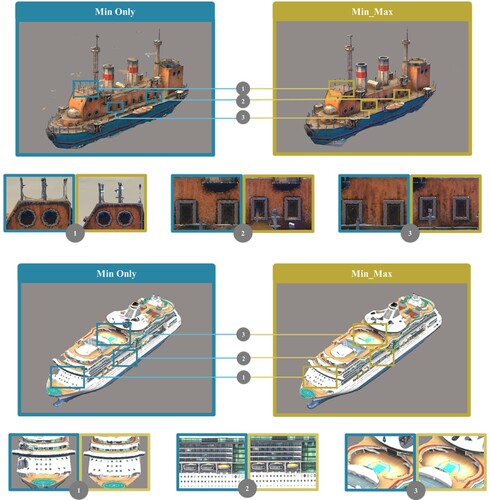
Min–Max strategy verification. Our method adopts a two-step strategy similar to the method in Zhou et al. (2020) to optimize the view set. In order to verify the effectiveness of the two-step strategy, we conducted an ablation experiment to compare the reconstruction result before and after the implementation of the two-step strategy. Table 2 shows the quantitative evaluation of the final reconstruction results. It should be noted that the maximization calculation will not change the scale of the view set. It only performs the replacement operation. The reason why the number of views is different in the second experiment group is due to the genetic algorithm used to generate the traversal path of the viewpoints. The position of the starting and ending viewpoints is uncertain due to the view replacement operation in the maximization calculation. When the starting and ending viewpoints are located on the same proxy model surface, the transition path will have an additional segment compared with the opposite case. Finally, this will lead to a different number of viewpoints on the two-step strategy. According to the experiment results, the implementation of the two-step strategy has significantly improved the reconstructability of the view set, meanwhile, the maximization calculation will take less time and the reconstruction error will decrease. However, the view redundancy has also increased to a certain extent. The ablation experiment shows that the two-step strategy can improve the reconstruction performance of view set.

Table 2. The adaptability verification of our method.

Scene	Method	Image number	$\mathcal{H}\left(\mathit{S},\mathit{U}\right)$	$\mathcal{R}\left(\mathit{U}\right)$	Time (s)	Reconstruction error
Stylized Ship	Min-Only	62	63.21747	0.21605	3.141	2.95446
	Max-Min	62	71.99685	0.40057	3.514	2.78677
Cruise Ship	Min-Only	66	37.43621	0.16458	4.047	4.17607
	Max-Min	77	61.30011	0.34455	4.959	5.35366

As shown in Figure 7, the left box shows the reconstruction result obtained only through the minimization calculation, and the right box shows the reconstruction result obtained through the Min–Max strategy. The comparison of the zoomed-in views shows that the details can be better recovered by the Min–Max strategy.

Figure 7. Reconstruction result of the ablation experiment.

WRP verification. In order to verify the effectiveness of WRP, we generate two different types of WRP for three times and compare the reconstruction results.

In the virtual scene, we simulate and generate two types of WRP based on the same initial path without wind disturbance (the number of viewpoints is 49 and the reconstruction error of the path is 3.18501). For the same kind of WRP, we set different thresholds to judge whether the offset viewpoint can be accepted. The maximum number of iterations of our algorithm is set to 1000.

As shown in Table 3, the viewpoint offset rate on the WRP generally increases with the threshold relaxation, meanwhile, the viewpoint offset rate of the ISWRP is significantly lower than that of the SWRP. In terms of the reconstruction error, the reconstruction error of the ISWRP is slightly less than that of the SWRP. In terms of time cost, due to the high viewpoint offset rate of the SWRP, the efficiency of the SWRP algorithm is generally lower than that of the ISWRP. However, a higher viewpoint offset rate means a better ability of wind resistance. Therefore, the SWRP will have better environment adaptability than the ISWRP.

Table 3. Comparison of the different types of WRP.

WRP type	Trail no.	Threshold	Offset rate	Position offset	Rotation offset	Time (s)	Reconstruction error
ISWRP	1	0.20	8.163%	20.44212	77.52457	3.425	3.14798
	2	0.25	16.33%	37.31263	147.91480	41.329	3.12878
	3	0.30	28.57%	56.96717	269.9075	79.282	3.01412
SWRP	1	0.20	97.96%	204.3250	799.0722	313.141	3.2226
	2	0.25	95.92%	201.4176	785.0208	341.547	3.1744
	3	0.30	100%	207.8728	788.8271	297.169	3.27652

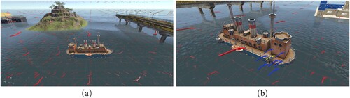
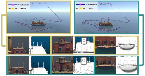
The two types of WRP in the virtual scene are shown in Figure 8. The threshold used to judge whether the offset viewpoint can be accepted is set to 0.3. The dashed line path represents the WRP generated by our algorithm, the solid line path represents the initial path without wind disturbance. The left box represents the effect of ISWRP, and the right box represents the effect of SWRP. The 3D models reconstructed based on the view sets captured by the two types of WRP are shown in Figure 8. From the perspective of the reconstruction result, both two WRPs can achieve a stable reconstruction. The difference is that the former takes less time than the latter.

Figure 8. Reconstruction effect of the two types of WRP. The left line border represents the effect of ISWRP, and the right line border represents the effect of SWRP.

We conducted several groups of controlled experiments to verify the initial stability of our WRP. As shown in Table 4, we randomly offset each viewpoint on the initial path without wind disturbance and repeat the experiment for five times. Then we use the view set generated by the path to reconstruct the ship. It can be found that the two types of WRP generated by our method can achieve a better reconstruction result compared with the path without wind disturbance. The fifth column in Table 4 shows the time cost of generating WRP. The offset of ISWRP is relatively small, and ISWRP is less time-consuming. It is more suitable for relatively stable wind field conditions.

Table 4. Initial stable verification of WRP.

Route type	Trail no.	Position offset	Rotation offset	Time (s)	Reconstruction error
No Wind Disturbance Resistance Path	1	201.4664	606.6971	/	3.70727
	2	200.3973	593.5197	/	3.54705
	3	211.4586	668.9821	/	3.68358
	4	213.7292	511.1758	/	3.77493
	5	193.9438	478.0896	/	3.48076
ISWRP	3	56.96717	269.9075	79.282	3.01412
SWRP	3	207.8728	788.8271	297.169	3.27652

In order to verify the self-stability of our WRP, we also conducted several groups of controlled experiments. As shown in Table 5, we take the SWRP path as the reference and carry out the offset operation of viewpoints. We repeat the experiment for five times. It can be seen that although the SWRP is offset, the final reconstruction error is almost the same as that of the original SWRP. This proves that the SWRP generated by our method has a strong ability of wind resistance. It is more suitable for complex wind field conditions.

Table 5. Initial stable verification of WRP.

Route type	Trail no.	Position offset	Rotation offset	Time (s)	Reconstruction error
SWRP	3	207.8728	788.8271	297.169	3.27652
Secondary offset on the SWRP	1	181.3021	504.9013	/	3.32948
	2	151.2565	536.5615	/	3.12584
	3	141.3802	621.5223	/	3.18620
	4	148.8815	642.9053	/	3.32917
	5	156.3399	515.0756	/	3.24366

5.3. Comparison with state-of-the-art

Necessity of adding transition path. In order to verify the necessity of adding transition path, we conducted a comparison experiment between our method and the method of Zhou et al. (2020). During the experiment, we use the same viewpoint setting in different methods (except the viewpoints on the transition path), and we quantitatively evaluate the reconstruction quality to verify the necessity of the transition path. Figure 9 clearly demonstrates the above conclusion.

Figure 9. Comparison between our method and the method of Zhou et al. (2020).

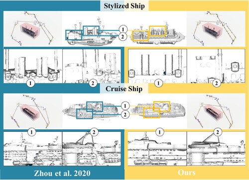
The comparison between our method and the method of Zhou et al. (2020) is shown in Table 6. The third column indicates the number of viewpoints on the UAV path and the number of views used for the reconstruction. The only difference between our method and the method of Zhou et al. (2020) lies in the presence or absence of a transition path. As shown in the fourth column, although the number of views generated by our method is more than that of the method of Zhou et al. (2020), the actual flight time of the UAV does not show a significant increase. As shown in the fifth column, our method can achieve a more stable reconstruction result based on the added transition path, while the method of Zhou et al. (2020) has a high probability of failure in reconstruction due to the lack of sufficient intersection between views.

Table 6. Comparison between our method and the method of Zhou et al. (2020).

Scene	Method	Image/adopt	Time (s)	Reconstruction error
Stylized Ship	Ours	57/57	178.893	3.11078
	Zhou et al. (2020)	41/32	176.586	Failed
Cruise Ship	Ours	54/54	144.255	2.3421
	Zhou et al. (2020)	38/31	143.837	Failed

Significance of model surface complexity. In order to verify the significance of introducing model surface complexity, we also conducted a comparison experiment between our method and the method of Zhou et al. (2020). We count the time cost of each step in our path planning algorithm and the reconstruction error.

As shown in Table 7, the fourth to sixth columns in the table represent the time cost of the view redundancy minimization calculation, reconstructability maximization calculation and the genetic algorithm for TSP problem. The eighth column represents the flight time of the UAV. It can be seen that our method performs better than the method of Zhou et al. (2020) based on the introduction of model surface complexity. The path length of our method is shorter than that of the method of Zhou et al. (2020). The time cost of our method is lower than that of the method of Zhou et al. (2020). Our method can effectively optimize the number of views according to the characteristics of ship, and improve the algorithm efficiency without affecting the reconstruction quality.

Table 7. Comparison between our method and the method of Zhou et al. (2020).

Scene	Method	Image num	Min (s)	Max (s)	TSP (s)	Length (m)	Flight (s)	Error
Stylized Ship	Ours	49	2.708	0.236	25.537	684.566	159.764	3.01325
	Zhou et al. (2020)	57	37.724	1.127	27.629	711.510	181.608	3.00785
Cruise Ship	Ours	54	2.919	0.231	25.656	720.245	142.290	2.45223
	Zhou et al. (2020)	62	75.773	3.461	33.114	747.415	172.492	2.66399

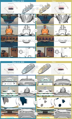
As shown in Figure 10, although our method uses fewer views than the method of Zhou et al. (2020), it is not inferior to the method of Zhou et al. (2020) in details of the reconstructed model.

Figure 10. Comparison of reconstruction result between our method and method in the method of Zhou et al. (2020). The right line border represents the effect of our method, and the left line border represents the effect of Zhou et al. 2020.

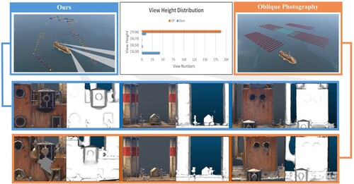
5.4. Comparison with oblique photography

As an aerial survey technology, the well-established oblique photography (OP) solution is widely used in the fields of engineering surveying and 3D modelling. In this section, we simulate OP solution to plan the UAV’s path in the virtual scene. OP generally adopts a five-camera UAV for image acquisition. We divide the path of the OP solution into five sub-paths. For each sub-path, we use a single-camera UAV to simulate the image acquisition. We use different parameters in each replicated experiment.

The comparison between our method and OP solution is shown in Table 8. The third to fifth columns represent the pitch angle, longitudinal overlap and side overlap of pan-tilt camera in OP solution, respectively. It can be seen from the table that OP solution is far inferior to our method in terms of route length and time cost. Although the reconstruction error of the OP solution is less than that of our method, our method achieves better results in some details. Our method can achieve a balance of efficiency and quality.

Table 8. The comparison between our method and OP solution.

Method	Images /adopt	Pitch (${}^{\circ }$)	Longitudinal overlap	Side overlap	Length (m)	Time (s)	Reconstruction error
Ours	56/56	/	/	/	728.780	171.641	2.92035
OP	447/240	60	0.7	0.75	1856.949	461.235	2.71720
	648/493	60	0.7	0.8	2666.632	631.727	Failed
	550/188	60	0.8	0.7	1554.192	384.766	2.54138

The OP solution usually adopts a fixed flight altitude. Therefore, it often fails to capture the surface details of the lower part of the object when reconstructing an object with a large height difference. As shown in Figure 11, the line border boxes represent the reconstruction results obtained by our method and the OP solution, respectively. The path planned by our method has no fixed height constraints. Our method can achieve high-quality 3D reconstructions. Although the number of images acquired by the OP solution is several times that of our method, the total image used in reconstruction is less than 50% of the number of images obtained by the OP solution.

Figure 11. The comparison between our method and OP solution. The left line border represents the effect of our method, and the right line border represents the effect of oblique photography.

6. Conclusion and future work

This paper proposes a UAV path planning method that takes into account both the image acquisition efficiency and the wind resistance. The time complexity of the overall algorithm is O(n²). The goal of our method is to reconstruct the ship target efficiently in wind-disturbed environments. Our method only needs to obtain the ship target’s AIS data to generate a cuboid proxy model. The wind resistance path will be generated based on the initial path without wind disturbance and the wind field model. Compared with the state-of-the-art method, our method calculates the characteristics of different surfaces of the ship target and optimizes the view set to reduce unnecessary views. Furthermore, our method introduces a wind resistance algorithm for the UAV to carry out efficient and high-quality reconstruction under a given wind situation.

As the power of the UAV decreases, the control performance and wind resistance ability of the UAV may also decrease. The relationship of wind speed, added energy consumption and consequential decrease autonomy is a very complex physical model. Our method does not directly analyse the above relationship. In this paper, we discuss the problem from the perspective of spatial geometry. The path scheme generated by our spatial geometry method can be completed by multiple rounds or multiple fully charged UAVs. Therefore, our method can be extended to multi-UAV system to perform the inspection in a high 3D reconstruction precision case.

Our method can realize the offline planning of the whole process. However, there are some limitations to its use. First of all, our method is focused on the reconstruction of single ship. For ship-intensive area, such as port, our method cannot ensure high reconstruction accuracy of all ships in the scene. Moreover, we assume a stable wind field model during the path optimization. In the future, we will attempt to explore the path planning method under the dynamic wind field model based on our proposed framework.

Disclosure statement

No potential conflict of interest was reported by the author(s).

Data availability statement

The data that support the findings of this study are available from the corresponding author, upon reasonable request.

Additional information

Funding

This work was supported by the National Natural Science Foundation of China [grant numbers 52071201 and 61602426]; Special Funding for the Development of Science and Technology of Shanghai Ocean University [grant number A2-2006-21-200207]; Fund of Hubei Key Laboratory of Inland Shipping Technology [grant number NHHY2019001]; Open Project Program of the State Key Lab of CAD&CG (Zhejiang University) [grant number A2107]; Open Subject of the State Key Laboratory of Engines (Tianjin University) [grant number K2019-14]; and Soybean Intelligent Computing Breeding and Application [grant number 2021PE0AC04].

References

- Arce, S., C. A. Vernon, J. Hammond, V. Newell, J. Janson, K. W. Franke, and J. D. Hedengren. 2020. “Automated 3D Reconstruction Using Optimized View-Planning Algorithms for Iterative Development of Structure-from-Motion Models.” Remote Sensing 12 (13): 2169.
- Cai, W., J. She, M. Wu, and Y. Ohyama. 2019. “Disturbance Suppression for Quadrotor UAV Using Sliding-Mode-Observer-Based Equivalent-Input-Disturbance Approach.” ISA Transactions 92: 286–297.
- Dai, B., Y. He, G. Zhang, F. Gu, L. Yang, and W. Xu. 2020. “Wind Disturbance Rejection for Unmanned Aerial Vehicles Using Acceleration Feedback Enhanced H∞ Method.” Autonomous Robots 44 (7): 1271–1285.
- Danilina, N., M. Slepnev, and S. Chebotarev. 2018. “Smart City: Automatic Reconstruction of 3D Building Models to Support Urban Development and Planning.” 6th International Scientific Conference on Integration, Partnership and Innovation in Construction Science and Education (IPICSE-2018), November 14–16, 251: 03047.
- Drešček, U., F. M. Kosmatin, J. Tekavec, and A. Lisec. 2020. “Spatial ETL for 3D Building Modelling Based on Unmanned Aerial Vehicle Data in Semi-Urban Areas.” Remote Sensing 12 (12): 1972.
- Furukawa, Y., and C. Hernández. 2015. Multi-View Stereo: A Tutorial, Foundations and Trends® in Computer Graphics and Vision. Hanover, MA: now Publishers Inc.
- Guo, K., J. Jia, X. Yu, L. Guo, and L. Xie. 2020. “Multiple Observers Based Anti-Disturbance Control for A Quadrotor UAV Against Payload and Wind Disturbances.” Control Engineering Practice 102: 104560.
- Hardouin, G., J. Moras, F. Morbidi, J. Marzat, and E. M. Mouaddib. 2021. “Next-Best-View Planning for Surface Reconstruction of Large-Scale 3D Environments with Multiple UAVs.” 2020 IEEE/RSJ International Conference on Intelligent Robots and Systems (IROS), Las Vegas, NV, USA, January 21–24.
- Hepp, B., M. Nießner, and O. Hilliges. 2018. “Plan3d: Viewpoint and Trajectory Optimization for Aerial Multi-View Stereo Reconstruction.” ACM Transactions on Graphics (TOG) 38 (1): 1–17.
- Hermann, M., B. Ruf, and M. Weinmann. 2021. “Real-time Dense 3D Reconstruction from Monocular Video Data Captured by Low-Cost UAVs.” ISPRS - International Archives of the Photogrammetry, Remote Sensing and Spatial Information Sciences 43B2: 361–368.
- Huang, R., D. Zou, R. Vaughan, and P. Tan. 2018. “Active Image-based Modeling with A Toy Drone.” 2018 IEEE International Conference on Robotics and Automation (ICRA), Brisbane, Australia, May 21–26.
- Jin, J., and N. L. Miller. 2007. “Analysis of the Impact of Snow on Daily Weather Variability in Mountainous Regions Using MM5.” Journal of Hydrometeorology 8 (2): 245–258.
- Jing, W., J. Polden, P. Y. Tao, W. Lin, and K. Shimada. 2016. “View Planning for 3D Shape Reconstruction of Buildings with Unmanned Aerial Vehicles.” 2016 14th International Conference on Control, Automation, Robotics and Vision (ICARCV), Phuket, Thailand, November 13–15.
- Koch, T., M. Körner, and F. Fraundorfer. 2019. “Automatic and Semantically-Aware 3D UAV Flight Planning for Image-Based 3D Reconstruction.” Remote Sensing 11 (13): 1550.
- Kuang, Q., J. Wu, J. Pan, and B. Zhou. 2020. “Real-Time UAV Path Planning for Autonomous Urban Scene Reconstruction.” 2020 IEEE International Conference on Robotics and Automation (ICRA), Virtual Conference, May 31 to June 15.
- Li, M., L. Nan, N. Smith, and P. Wonka. 2016. “Reconstructing Building Mass Models from UAV Images.” Computers & Graphics 54: 84–93.
- Li, F., M. Song, J. Chi, and Y. Cheng. 2021a. “Ship Velocity Estimation via Images Acquired by An Unmanned Aerial Vehicle-Based Hyperspectral Imaging Sensor.” Journal of Applied Remote Sensing 15 (3): 032206.
- Liu, Y., R. Cui, K. Xie, M. Gong, and H. Huang. 2021b. “Aerial Path Planning for Online Real-Time Exploration and Offline High-Quality Reconstruction of Large-Scale Urban Scenes.” ACM Transactions on Graphics (TOG) 40 (6): 226.
- Liu, J., X. Lu, C. Peng, and J. Ma. 2021a. “Adaptive RBF Neural Network Control of A Small-scale Coaxial Rotor Unmanned Aerial Vehicle.” 40th Chinese Control Conference (CCC), Shanghai, China, July 26–28.
- Schmid, L., M. Pantic, R. Khanna, L. Ott, R. Siegwart, and J. Nieto. 2020. “An Efficient Sampling-Based Method for Online Informative Path Planning in Unknown Environments.” IEEE Robotics and Automation Letters 5 (2): 1500–1507.
- Schonberger, J. L., and J. M. Frahm. 2016. “Structure-from-Motion Revisited.” IEEE Conference on Computer Vision and Pattern Recognition, Las Vegas, NV, USA June 27 to June 30.
- Shen, L., Y. Wang, K. Liu, Z. Yang, X. Shi, X. Yang, and K. Jing. 2020. “Synergistic Path Planning of Multi-UAVs for Air Pollution Detection of Ships in Ports.” Transportation Research Part E: Logistics and Transportation Review 144: 102128.
- Shi, D., X. Dai, X. Zhang, and Q. Quan. 2017. “A Practical Performance Evaluation Method for Electric Multicopters.” IEEE/ASME Transactions on Mechatronics 22 (3): 1337–1348.
- Smith, N., N. Moehrle, M. Goesele, and W. Heidrich. 2018. “Aerial Path Planning for Urban Scene Reconstruction: A Continuous Optimization Method and Benchmark.” ACM Transactions on Graphics (TOG) 37 (6): 183.
- Suzuki, T., Y. Amano, T. Hashizume, and S. Suzuki. 2011. “3D Terrain Reconstruction by Small Unmanned Aerial Vehicle Using SIFT-Based Monocular SLAM.” Journal of Robotics and Mechatronics 23 (2): 292–301.
- Vogiatzis, G., and C. Hernández. 2011. “Video-based, Real-Time Multi-View Stereo.” Image and Vision Computing 29 (7): 434–441.
- Wang, R., Z. Zhou, X. Zhu, and Z. Wang. 2021. “Responses and Suppression of Joined-Wing UAV in Wind Field Based on Distributed Model and Active Disturbance Rejection Control.” Aerospace Science and Technology 115: 106803.
- Wen, J., H. Wang, and D. Li. 2020. “Anti-wind Trajectory Control for Unmanned Aerial Vehicle with Nonlinear Dynamic Inversion Based on High Order Sliding Mode.” 2020 3rd International Conference on Unmanned Systems (ICUS), Harbin, China, November 27–28.
- Wu, C. 2013. “Towards Linear-time Incremental Structure from Motion.” 2013 International Conference on 3D Vision-3DV, Seattle, WA, USA. June 29 to July 1.
- Xi, H., D. Zhang, T. Zhou, Y. Yang, and Q. Wei. 2021. “An Anti-Wind Modeling Method of Quadrotor Aircraft and Cascade Controller Design Based on Improved Extended State Observer.” International Journal of Control, Automation and Systems 19 (3): 1363–1374.
- Xu, Z., L. Wu, M. Gerke, R. Wang, and H. Yang. 2016. “Skeletal Camera Network Embedded Structure-from-Motion for 3D Scene Reconstruction from UAV Images.” ISPRS Journal of Photogrammetry and Remote Sensing 121: 113–127.
- Yan, F., E. Xia, Z. Li, and Z. Zhou. 2021. “Sampling-based Path Planning for High-Quality Aerial 3D Reconstruction of Urban Scenes.” Remote Sensing 13 (5): 989.
- Yang, B., F. Ali, B. Zhou, S. Li, Y. Yu, T. Yang, X. Liu, Z. Liang, and K. Zhang. 2022. “A Novel Approach of Efficient 3D Reconstruction for Real Scene Using Unmanned Aerial Vehicle Oblique Photogrammetry with Five Cameras.” Computers and Electrical Engineering 99: 107804.
- Yuan, H., C. Xiao, Y. Wang, X. Peng, Y. Wen, and Q. Li. 2020. “Maritime Vessel Emission Monitoring by an UAV Gas Sensor System.” Ocean Engineering 218: 108206.
- Zhang, Bo. 2020. “Research on the Control System of Quadrotor UAV under Wind Interference.” M.S. diss., Taiyuan University of Technology (TYUT).
- Zhang, H., Y. Yao, K. Xie, C. W. Fu, H. Zhang, and H. Huang. 2021. “Continuous Aerial Path Planning for 3D Urban Scene Reconstruction.” ACM Transactions on Graphics (TOG) 40 (6): 225.
- Zhang, Q., J. Zhang, X. Wang, Y. Xu, and Z. Yu. 2020. “Wind Field Disturbance Analysis and Flight Control System Design for A Novel Tilt-Rotor UAV.” IEEE Access 8: 211401–211410.
- Zhang, C., X. Zhou, H. Zhao, A. Dai, and H. Zhou. 2016. “Three-Dimensional Fuzzy Control of Mini Quadrotor UAV Trajectory Tracking under Impact of Wind Disturbance.” 2016 International Conference on Advanced Mechatronic Systems (ICAMechS), Melbourne, VIC, Australia, November 30 to December 03.
- Zheng, X., F. Wang, and Z. Li. 2018. “A Multi-UAV Cooperative Route Planning Methodology for 3D Fine-Resolution Building Model Reconstruction.” ISPRS Journal of Photogrammetry and Remote Sensing 146: 483–494.
- Zhou, F., S. Pan, and J. Jiang. 2019. “Verification of AIS Data by Using Video Images Taken by A UAV.” The Journal of Navigation 72 (6): 1345–1358.
- Zhou, X., K. Xie, K. Huang, Y. Liu, Y. Zhou, M. Gong, and H. Huang. 2020. “Offsite Aerial Path Planning for Efficient Urban Scene Reconstruction.” ACM Transactions on Graphics (TOG) 39 (6): 192.