Hyperspectral anomaly detection: a performance comparison of existing techniques

ABSTRACT

Anomaly detection in Hyperspectral Imagery (HSI) has received considerable attention because of its potential application in several areas. Numerous anomaly detection algorithms for HSI have been proposed in the literature; however, due to the use of different datasets in previous studies, an extensive performance comparison of these algorithms is missing. In this paper, an overview of the current state of research in hyperspectral anomaly detection is presented by broadly dividing all the previously proposed algorithms into eight different categories. In addition, this paper presents the most comprehensive comparative analysis to-date in hyperspectral anomaly detection by evaluating 22 algorithms on 17 different publicly available datasets. Results indicate that attribute and edge-preserving filtering-based detection (AED), local summation anomaly detection based on collaborative representation and inverse distance weight (LSAD-CR-IDW) and local summation unsupervised nearest regularized subspace with an outlier removal anomaly detector (LSUNRSORAD) perform better as indicated by the mean and median values of area under the receiver operating characteristic (ROC) curves. Finally, this paper studies the effect of various dimensionality reduction techniques on anomaly detection. Results indicate that reducing the number of components to around 20 improves the performance; however, any further decrease deteriorates the performance.

KEYWORDS:

• Anomaly detection algorithms
• hyperspectral imagery
• deep learning
• dimensionality reduction

1. Introduction

In recent years, hyperspectral imaging has gained a lot of attention because of its spectral and spatial resolution (Goetz et al. 1985). Its spectral information ranges from visual band to far-infrared spectrum and provides a spectral curve of materials (Fauvel et al. 2013; Tao et al. 2019). In HSI, each image is a multi-spectral cube that has two spatial dimensions and one spectral dimension. The spectral dimension contains a high-dimensional reflectance vector (Li et al. 2018; Xie et al. 2019a). Depending on the HSI sensor, the hyperspectral data cube can be composed of several hundred spectral bands, each band with a narrow range of wavelengths, i.e. 10–20 nm. Due to the high information content in its spectral bands, HSI is used in applications, such as remote sensing (Khan et al. 2018). HSI can also distinguish between different materials based on their spectral signatures (Li et al. 2018). This property is exploited in various applications (Xie et al. 2019a) such as image classification (Camps-Valls and Bruzzone 2005; Harsanyi and Chang 1994), minerals detection (Reed and Yu 1990), tracking changes in the environment (Bioucas-Dias et al. 2012; Theiler and Wohlberg 2012) and anomaly detection (Reed and Yu 1990; Stein et al. 2002) etc.

Anomaly detection is a notable application where HSI-based techniques have been applied recently (W. Zhang, Lu, and Li 2019). Anomalies are the pixels whose spectral signature is different from the background (Chalapathy and Chawla 2019). In some contexts, these anomalies are referred to as targets that appear different from the background either spatially or spectrally. Anomaly detection is a binary classification problem that does not require prior knowledge of anomalies (Matteoli, Diani, and Corsini 2010; Qu et al. 2018; Zhao, Du, and Zhang 2014), where pixels with different spectral signatures are labeled as anomalies and the remaining pixels are treated as background (Yuan, Wang, and Zhu 2015). In general, anomalies have a low chance of occurrence, and these are typically small objects (W. Zhang, Lu, and Li 2019). Hence, the basic goal is to detect targets with distinguishable spectra from the background (Li et al. 2018).

Anomaly detection using HSI has gained significant attention due to its use in military and civilian applications. These application areas include defense (Kiran, Thomas, and Parakkal 2018), agronomy (Waheed et al. 2006; Yang et al. 2014), safety (Makki et al. 2017), minerals detection (Bioucas-Dias et al. 2012; Reed and Yu 1990), environmental monitoring (Bioucas-Dias et al. 2012; Chen et al. 2018) and medical applications (Baur et al. 2018; Seeböck et al. 2016). NASA’s Mars rover uses a 12-band multispectral stereo camera for capturing images and anomaly detection is subsequently applied to identify anomalies of interest (Ayhan et al. 2017). Some other anomalies of interest in real-world scenarios include a ship in the sea, a vehicle in the forest and an airplane in the sky. The goal is to identify and distinguish unusual objects from the background without explicitly defining the objects beforehand.

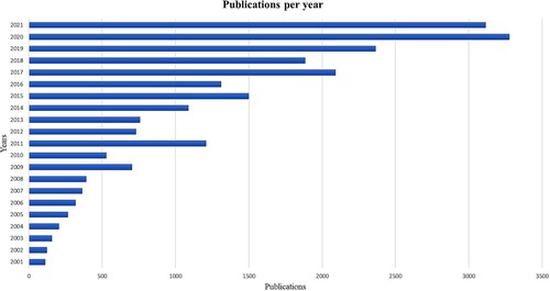
Figure 1 shows the total number of published articles related to anomaly detection in hyperspectral images. The statistics for each year indicate the articles published in that year. For more detailed insights on the statistics of publications done in this area, the readers may refer to this article (Racetin and Krtalić 2021).

Figure 1. Annual publications per year from 2000 to 2021.

The objective of anomaly detection is to identify a small number of pixels in the hyperspectral image whose spectral properties are distinct from the rest of the pixels whereas the target detection a.k.a. spectral matching detection seeks to locate pixels whose spectrum demonstrates a strong correlation to the desired signature (Manolakis 2005; Matteoli, Diani, and Corsini 2010; Nasrabadi 2014).

Hyperspectral anomaly detection techniques face several challenges (Salem, Ettabaa, and Hamdi 2014). The first challenge is to decrease the false alarm rate while increasing the detection accuracy, which is intricate due to contamination of background statistics and the presence of noise in anomaly signatures. Another challenge is to detect anomalies of various sizes and shapes. Anomalies can vary in size from sub-pixel to a few pixels. Therefore, the detection of these anomalies with varying sizes using the same detector becomes a difficult task. The third challenge is to perform anomaly detection using real-time processing on platforms with computation constraints. The selection of parameters for different techniques is another challenge as the parameters of a technique vary with the size of the anomaly. Due to these challenges, anomaly detection has remained a topic of active research over the past two decades.

An overview of the literature shows that hyperspectral anomaly detection has been proposed using several techniques such as statistical techniques, filtering techniques, clustering techniques, subspace techniques and more recently, deep learning techniques. Unfortunately, due to the use of different datasets in different studies, a comparison of different algorithms cannot always be made. Recently, Su et al. (2022) have also surveyed anomaly detection for HSI, however, they have done performance evaluation of nine algorithms using only three datasets, whereas we have done performance evaluation of 22 algorithms on 17 datasets. Moreover, we have also investigated the effect of dimensionality reduction on anomaly detection performance.

1.1. Contributions

The contributions of this paper are threefold.

• First, this paper provides an overview of the current state of research in hyperspectral anomaly detection. For this purpose, we divide the anomaly detection techniques into eight broad categories and discuss the progress made in each category.

• Second, this paper provides a comprehensive performance comparison of hyperspectral anomaly detection algorithms to-date by comparing 22 anomaly detection algorithms on 17 different publicly available datasets. For this purpose, both the area under the receiver operating characteristic (ROC) curve as well as the execution times are compared. Results show that edge-preserving filtering-based techniques (Kang et al. 2017) provide an optimal combination of detection performance and execution time.

• Finally, this paper studies the effect of dimensionality reduction on anomaly detection performance. Due to the large size of the hyperspectral data cube, it is common to employ dimensionality reduction techniques for pre-processing in many applications. However, reducing the spectral dimensions of the data cube can also remove anomalies. For this purpose, the detection performance of the classic Reed-Xiaoli detector (Reed and Yu 1990) on dimension-reduced data is evaluated. Results show that, in general, reducing the number of components to around 20 improves anomaly detection performance. However, depending on the data, a further decrease in the number of components can cause a significant deterioration in performance.

The remaining paper is organized as follows. Section 2 describes various types of anomalies and the basic principle of different techniques used for anomaly detection. Section 3 reviews the published work based on different categories of anomaly detection techniques. Section 4 describes the commonly used datasets in reviewed publications. In Section 5, we evaluate and discuss the performance of existing algorithms on hyperspectral datasets. Section 6 describes our simulation results for different dimensionality reduction techniques on hyperspectral datasets.

2. Types of anomalies and system models

This section describes the types of anomalies and the system models for anomaly detection. The type of anomaly detection algorithm used in an application is heavily influenced by the nature of the anomaly. Hyperspectral anomalies can be divided into three categories; sub-pixel anomaly, pixel anomaly and multiple pixels anomalies (Du et al. 2016).

Sub-pixel anomalies are targets that only take up a small portion of a pixel. From a physical perspective, a subpixel anomaly is often heavily mixed with its neighbors in majority of spectral areas of its pixel spectrum (Huang, Fang, and Li 2020; Khazai et al. 2013). However, there is a very high possibility that a subpixel anomaly, particularly a synthetic one, will influence some spectral areas of its pixel spectra. Certain anomalous pixels of small objects such as vehicles or mineral stones that only take up one or fewer pixels are referred to as single-pixel anomaly targets (Du et al. 2016; Racetin and Krtalić 2021). Likewise, anomalous targets that consist of multiple pixels that are lumped together are known as multi-pixel anomaly targets (Liu et al. 2022). Vehicles and airplanes in an airport are examples of single and multi-pixel anomalies respectively (Du et al. 2016).

2.1. Signal model

Consider a hyperspectral image, x ∈ ℝ^a × N where a is a pixel location and N is the number of spectral bands. The anomaly detection problem can be formulated as a binary composite hypothesis testing problem: (1) $\begin{array}{c}{\mathrm{H}}_0:x=b\mathrm{A}\mathrm{n}\mathrm{o}\mathrm{m}\mathrm{a}\mathrm{l}\mathrm{y}\mathrm{a}\mathrm{b}\mathrm{s}\mathrm{e}\mathrm{n}\mathrm{t}\\ {\mathrm{H}}_1:x=b+as\mathrm{A}\mathrm{n}\mathrm{o}\mathrm{m}\mathrm{a}\mathrm{l}\mathrm{y}\mathrm{p}\mathrm{r}\mathrm{e}\mathrm{s}\mathrm{e}\mathrm{n}\mathrm{t}\end{array}$(1) where $a=0$ under H₀ and $a>0$ under H₁ . $b$ is the background clutter and $s$ is the spectral signature of the anomaly. Unlike the target detection problem where the distribution of the target is assumed to be known, in an anomaly detection no prior information about anomalies is available. Therefore, it can be viewed as a problem of checking whether each pixel spectra belongs to the background distribution or not. Hence, the first step of an anomaly detection problem is to estimate the background probability distribution. In the literature, multiple algorithms have been proposed utilizing both model-based and non-model-based estimators. For example, Gaussian (Reed and Yu 1990) and Gaussian mixture models (Reynolds 2009) are both popular distributions used to model the background. Similarly, Clustering (Carlotto 2005), Support Vector Machine (Noble 2006), Random Forest (Pal 2005) and Neural Networks (Atkinson and Tatnall 1997) are some examples of non-model-based techniques (Gao et al. 2018).

Depending on the method used for background estimation, anomaly detection algorithms can be broadly classified as either global or local algorithms. In global anomaly detection algorithms, the background is estimated from the complete hyperspectral data cube available before testing individual pixels. On the contrary, in local algorithms, the background is estimated using neighbors of the pixel under test. As a result, local anomaly detection algorithms are typically more computationally intensive compared to their global counterpart.

3. Anomaly detection algorithms

Different techniques have been proposed in previous studies for anomaly detection in hyperspectral imagery. Classical techniques include statistics-based (Guo et al. 2014; Liu and Chang 2004; Reed and Yu 1990), subspace-based (Li and Du 2013; Schaum 2004), kernel-based (Banerjee, Burlina, and Diehl 2006; Kwon and Nasrabadi 2005) and clustering-based approaches (Carlotto 2005; Hytla et al. 2009). More recent techniques include filtering-based (Kang et al. 2017; Li et al. 2018), low-rank-based (Qu et al. 2018; Xu et al. 2016; Zhou and Tao 2011) and representation-based (Li and Du 2015; Wang et al. 2020) approaches that have gained attention due to their capability of separating the anomalies and background. Deep unsupervised learning (Ma et al. 2018; Zhang and Cheng 2019) has also been used recently and has been shown to yield good results for anomaly detection. These eight categories of anomaly detection algorithms are discussed next.

3.1. Statistics-based techniques

In 1990, Reed and Yu (1990) proposed the classic anomaly detection algorithm, commonly known as RX (Reed-Xiaoli) detector, which is based on the modeling of background as a multivariate Gaussian distribution. In particular, the test hypothesis in the RX detector (Reed and Yu 1990) is defined as follows: (2) $T\left(\mathit{x}\right)=(\mathit{x}-\hat{\mathit{\mu }}{)}^T{\hat{\mathit{C}}}^{-1}(\mathit{x}-\hat{\mathit{\mu }}),$(2) where $\mathit{x}$ is the pixel under test, $\hat{\mathit{\mu }}$ and $\hat{\mathit{C}}$ are the estimated mean and covariance of the background data respectively. If the test statistic, $T\left(\mathit{x}\right)$, exceeds a threshold, the pixel under test is declared an anomaly. Both $\hat{\mathit{\mu }}$ and $\hat{\mathit{C}}$ are estimated from the available data cube using the sample mean and sample covariance, (3) $\hat{\mathit{\mu }}={\displaystyle \frac{1}{n}\sum _{i=1}^n{\mathit{x}}_i,}$(3) (4) $\hat{\mathit{C}}={\displaystyle \frac{1}{n}\sum _{i=1}^n\left({\mathit{x}}_i-\hat{\mathit{\mu }}\right)({\mathit{x}}_i-\hat{\mathit{\mu }}{)}^T,}$(4) where $n$ is the number of pixels used for background estimation. In the global RX detector, the complete data cube is used for background estimation, therefore, $n$ represents the total number of pixels in the data cube.

One of the limitations of this global RX detector is that a multivariate Gaussian distribution is not sufficient to model the entire background statistics (Tan et al. 2019). It also leads to contamination since target pixels are also included in the calculations of background statistics (Tu et al. 2020a; Zhao, Du, and Zhang 2014).

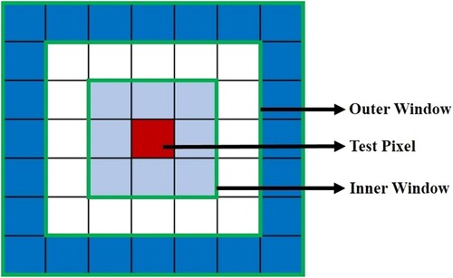
To overcome this limitation, a local RX detector is proposed (Reed and Yu 1990). This detector is a mixture of multivariate Gaussian models. It uses a local double concentric window that slides over the entire hyperspectral image to get the local background statistics. It consists of two windows: the inner and outer windows. The outer window is used to calculate the mean and covariance matrix in the local regions and the inner window is used to avoid the anomaly pixels while calculating the background statistic in the outer window. However, this detector is computationally expensive because the sliding window calculates the covariance matrix at each test pixel location (Banerjee, Burlina, and Diehl 2006; Zhao et al. 2015).

Unlike the local RX detector that uses the inner window to avoid anomaly pixels in the calculation of background statistics, the dual window RX detector (Liu and Chang 2004) uses the difference between the inner window and outer window, which is known as a guard band. The guard band is used to maximize the separation between the background and anomalies. The mean of the guard band and the local covariance matrix is used for the detection of anomalies. LRX detector uses a guard band to avoid the pixel under test from encroaching into the estimation of background information. Whereas DWRX makes use of this guard band data in contrast to the LRX. Instead of utilizing the test pixel's spectra, it utilizes the average spectral pixels that lie within the guard band. One of the limitations of the dual and local window RX detector is that the size of the inner window must be equal to or greater than the size of an anomaly (Küçük and Yüksel 2015). Therefore, these methods require information about the size of anomalies but they may not be accessible (Qu et al. 2018).

Liu and Chang (2013) proposed a technique based on multiple windows to detect anomalies of varied sizes. The multiple windows consist of the inner, middle and outer windows. The technique uses multiple windows of different sizes to estimate the covariance of background within a local region. Different detection maps are generated which are combined to detect the anomalies by using a threshold. However, selecting suitable multiple windows depend upon the size of anomalies.

In a weighted RX detector (Guo et al. 2014), different weights are assigned to pixels according to the distance from the background. If the pixel under consideration is distant from the background, then it is assigned a lower weight in the background estimation, otherwise, the pixel is assigned a higher weight. While estimating the background, anomalous pixels and noisy pixels are eliminated as the background assumes a multivariate Gaussian distribution.

Du and Zhang (2011) proposed an anomaly detection algorithm based on the random selection of background pixels. First, background information is randomly selected from the hyperspectral image. Then, several random selections are repeatedly made to acquire different statistics of background, thereby reducing the contamination of anomalies in the background statistics. This algorithm also tries to separate the background information from anomalous pixels. Liu and Han (2017) proposed a method based on the spectral derivative. First, the spectral derivative filter is applied to capture the fine structure of the spectra which is followed by the RX detector. This algorithm gave better performance than the RX detector as it captured the fine structure of the data instead of directly applying the RX to hyperspectral data. Tao et al. (2019) proposed a Fractional Fourier Entropy RX technique to better discriminate between anomaly and background pixels. First, the Fractional Fourier transform is used as a preprocessing step to take the advantage of an intermediate domain to find the features between the reflectance spectrum and Fourier transform information. Then Fractional Fourier entropy-based strategy is used to automatically determine the optimal fractional order. The optimal fractional order produces detailed information in the image which increases the discrimination between background and anomaly pixels. Lastly, the RX detector is applied to detect the anomaly.

Sun et al. (2021) proposed a binary tree-based structure to extract features of background and targets. Separation is calculated via binary encoding based on the tree structure. As its target detection technique, therefore prior spectrum is also required. Ensemble-based information retrieval with mass estimation (EIRME) is proposed for hyperspectral target detection (Sun et al. 2022), however, this algorithm requires prior target spectrum. This framework utilizes a tree like structure to make feature space from which information retrieval is done for target detection.

3.2. Subspace-based techniques

The selection of windows for the estimation of background heavily influences anomaly detection performance in statistical detectors. A modified version of the RX detector, known as the Subspace RX detector, is proposed to reduce the constraints of window sizes (Schaum 2004). This approach assumes that the anomaly and background spectra can be expressed in different subspaces. The signal model for the $N$-dimensional background spectra can be formulated as (5) $\mathit{x}=\mathit{B}\hat{\mathit{S}}+\mathit{n},$(5) where the column space of $\mathit{B}$ spans the $p$-dimensional background subspace in the presence of white Gaussian noise. As the anomaly spectra are not known a-priori, it is assumed that the anomaly spectra do not lie in this background subspace.

The autocorrelation matrix of the background pixels can be expressed as (6) ${\hat{\mathit{R}}}_{\mathit{x}}=\mathit{B}{\hat{\mathit{R}}}_s{\mathit{B}}^H+{\sigma }^2\mathit{I},$(6) where ${\hat{\mathit{R}}}_s=E\left[\mathit{S}{\mathit{S}}^H\right]$ represents the autocorrelation matrix of $\hat{\mathit{S}}$. In practice, this correlation matrix would be estimated from the hyperspectral data. Signal subspace techniques typically rely on the eigenspace of the correlation matrix ${\hat{\mathit{R}}}_{\mathit{x}}$ to identify the background subspace. The eigenvectors of ${\hat{\mathit{R}}}_{\mathit{x}}$, $\left\{{\mathit{v}}_1,{\mathit{v}}_2,\dots ,{\mathit{v}}_p\right\}$, corresponding to the p-largest eigenvalues provide a basis for the background subspace while the remaining eigenvectors $\left\{{\mathit{v}}_{p+1},{\mathit{v}}_{p+2},\dots ,{\mathit{v}}_N\right\}$ provide a basis for the orthogonal subspace. Using these eigenvectors, matrices ${\hat{\mathit{W}}}_b$ and ${\hat{\mathit{W}}}_t$ can be defined as (7) ${\hat{\mathit{W}}}_b=\left[{\mathit{v}}_1{\mathit{v}}_2{\mathit{v}}_3\dots {\mathit{v}}_p\right],$(7) (8) ${\hat{\mathit{W}}}_t=\left[{\mathit{v}}_{\left(p+1\right)}{\mathit{v}}_{\left(p+2\right)}\dots {\mathit{v}}_N\right].$(8) In Complementary Subspace Detector (CSD) (Schaum 2007), the test statistic is defined as (9) $T\left(\mathit{x}\right)={\mathit{x}}_t^2-{\mathit{x}}_b^2.$(9) where ${\mathit{x}}_t$ and ${\mathit{x}}_b$ are the projections of $\mathit{x}$ on column space of ${\hat{\mathit{W}}}_t$ and ${\hat{\mathit{W}}}_b$, respectively. Similarly in the Subspace RX detector (Schaum 2004), the test pixel is first projected onto the background subspace to obtain ${\mathit{x}}_b$. The RX detector is then applied on ${\mathit{x}}_b$.

Li and Du (2013) presented an unsupervised nearest regularized subspace technique based on dual window strategy. Each pixel under consideration is linearly combined by surrounding pixels inside the outer window to estimate the new prediction of each test pixel. An assessment is used to get the similarity between the input and the new prediction pixel. Based on these values, anomalies are determined based on less similar values. This approach still produces high false alarms and selecting suitable dual windows depends upon the size of anomalies.

The local pixels may contain many anomalous pixels in the neighborhood which is one of the problems in many anomaly detection techniques. To separate the background and anomaly pixels, Li et al. (2015) proposed a technique based on joint sparse representation. First, a dictionary is constructed using similar spectra in the local neighborhood which belongs to the background information. At first, the background basis for the local region is selected. Then an unsupervised adaptive subspace detector is applied to check if the pixel under test is anomalous. The unsupervised adaptive subspace detector enhances the anomalies whereas the background is suppressed in the hyperspectral image. Therefore, the proposed algorithm detects anomalies in the complex background. However, the selection of parameters is different for each dataset.

The background is contaminated by anomaly pixels in the window-based technique (Du et al. 2016) and a single window cannot represent the complex local information of the background (Liu and Chang 2013). Du et al. (2016) proposed a technique based on local summation anomaly detection which takes into account both spectral and spatial information of the hyperspectral image to overcome these constraints. Initially, multiple windows are selected to get multiple normal distributions. The edge expansion is used as a preprocessing step. Then the sliding window is used to get the local covariance matrix which is projected to some other feature space to obtain the Mahalanobis distance of each local window. Then the initial detection results are obtained by adding the Mahalanobis distance of all the local windows. Lastly, binarization is used to get the final results. However, multiple sliding windows are time-consuming and computationally very expensive (Tan et al. 2019).

Tan et al. (2019) presented a technique to overcome the constraints in local summation anomaly detection. The method is called ‘the local summation unsupervised nearest regularize subspace with an outlier removal anomaly detector’. The basic idea of the first technique is to remove the outliers to improve detection accuracy. First, the outliers in the dual window are removed by using some predefined threshold. Then the strategy used in local summation anomaly detection is adopted using a dual window. Finally, the sliding dual window approach is also used to obtain accurate background information. However, this technique is still computationally expensive and the selection of parameters, such as constant $\lambda$ (regularization parameter), and the size of inner and outer windows are not constant for different datasets.

In go-decomposition (GoDec), a low-rank and sparsity-matrix decomposition (LRaSMD) method is used to find these matrices iteratively (Chang et al. 2021). The authors claim to achieve promising results on different datasets. Chang, Cao, and Song (2021) proposed an orthogonal subspace projector with go-decomposition (OSPGoDec) along with automatic target generation process. In this work, data sphering is utilized to make OS applicable to hyperspectral anomaly detection. Experiments indicate that this technique outperforms classical techniques like RX detector and collaborative representation-based anomaly detectors.

3.3. Kernel-based techniques

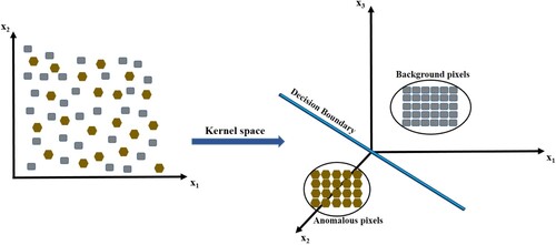
The fundamental idea behind the kernel-based technique is to transform the data spectra by mapping them to a high dimensional space where it is linearly separable. This is graphically depicted in Figure 2 where the anomaly and background spectra are not linearly separable but a linear decision boundary can be obtained after mapping to a higher dimension kernel space. Based on this concept, kernel-based detectors have been proposed in the literature which map each pixel into a higher dimensional space before applying a detector. Consider a hyperspectral image x $\in$ ${\mathbb{R}}^{m\times d}$ in which $m$ and $d$ are the numbers of pixels and bands respectively, the input image is mapped into a high dimensional feature $F$ using the mapping function ($\mathbf{\Phi }$) (Kwon and Nasrabadi 2005). (10) $\mathbf{x}\to \mathbf{\Phi }\left(\mathbf{x}\right).$(10) where $\mathit{x}$ is an input vector that is mapped into high-dimensional feature space by the kernel function $\mathbf{\Phi }$.

Figure 2. An illustration of the kernel-based algorithm in which input data is projected to high dimensional feature space.

A nonlinear RX detector is proposed using a kernel function (Kwon and Nasrabadi 2005). The proposed detector, referred to as Kernel RX detector, is defined as follows: (11) $T\left(\mathit{x}\right)=\left(\mathbf{\Phi }\right(\mathit{x})-{\mathbf{\Phi }}_{\hat{\mu }b}{)}^T{\hat{\mathit{K}}}_b^{-1}(\mathbf{\Phi }\left(\mathit{x}\right)-{\mathbf{\Phi }}_{\hat{\mu }b}),$(11) where $\mathbf{\Phi }\left(\mathit{x}\right)$ and ${\mathbf{\Phi }}_{\hat{\mu }b}$ represent the kernel mapping of the pixel under test and background means respectively and ${\hat{\mathit{K}}}_b$ denotes the calculated center Gram Matrix. Only a good choice for the kernel function $\mathbf{\Phi }$ is needed that can generate a positive definite Gram matrix. The Gaussian RBF is used as a kernel function in this technique (Scholkopf et al. 1997). If the test statistic, $T\left(\mathit{x}\right)$, exceeds a threshold, the pixel under test is declared an anomaly.

Different kernel functions (Souza 2010) are used in the literature, such as linear (Maji, Berg, and Malik 2008), polynomial (Smits and Jordaan 2002), Gaussian (Keerthi and Lin 2003), sigmoid (Hyperbolic Tangent) (Lin and Lin 2003) and Mahalanobis kernel (Hussain et al. 2011). Although the Gaussian radial basis function (RBF) (Scholkopf et al. 1997) is defined as (12) $\mathbf{K}\left({\mathit{x}}_i,{\mathit{x}}_j\right)=\mathrm{e}\mathrm{x}\mathrm{p}\left(-\gamma \parallel {\mathit{x}}_i-{\mathit{x}}_j{\parallel }^2\right),\gamma >0,$(12) is the most commonly used kernel in the literature, selecting a suitable kernel function is a challenging task and the kernel function’s complexity often leads to enormous amounts of computations as it estimates and inverts a large covariance matrix (Banerjee, Burlina, and Diehl 2006; Molero et al. 2012).

Banerjee, Burlina, and Diehl (2006) proposed a support vector data descriptor (SVDD) which is a nonparametric background model. It is a one-class support vector machine, capable of detecting anomalies that lie outside the support region. It avoids assumptions about data distribution which is modeled in previous RX detectors (Tu et al. 2019). It simply models the background using minimum enclosing hypersphere (MEH). MEH is achieved by using the kernel function (Schölkopf et al. 1999). Gaussian RBF is used as a kernel function that requires less computation. It maps the data to some high-dimensional space and calculates the inner product. Therefore, SVDD can calculate several support regions for data that can model multi-model distribution. It can detect anomalies with fewer false alarms.

KRX and SVDD are kernel feature space-based techniques and they are different from each other. SVDD is a discriminatory model that does not consider any distribution for the data. However, KRX is based on a generative model representing data as a Gaussian distribution. Moreover, KRX requires large computations as it estimates and inverts large covariance matrices whereas SVDD avoids this.

Zhao, Du, and Zhang (2014) developed a robust nonlinear detection technique that combines the concept of robust regression analysis and kernel-based learning. Initially, the hyperspectral data is projected to a suitable high-dimensional space. Normally distributed data is acquired from data during this feature space. Next, regression analysis is applied to the feature data for the repetitive corresponding generalized likelihood ratio test (GLRT) terms. Due to high dimensional feature space, the GLRT expression is first kernelized. Gaussian RBF is used as a kernel function in the proposed techniques. The objective of the technique is to avoid the calculation of anomalies in the background statistics. Zhou et al. (2016) proposed a cluster kernel RX (CKRX) technique that divides the hyperspectral image background into clusters and detects anomalies using a fast eigenvalue decomposition approach. In the clustering step, the pixels of the background are clustered and the relevant cluster centers are replaced. After that, the RX is applied to the samples, which results in reducing the computational cost.

Li et al. (2019) proposed a technique for hyperspectral anomaly detection which is based on isolation forest. Isolation forest is used for the first time to get the isolation feature of the anomaly. First, kernel principal component analysis (K-PCA) (Hoffmann 2007) is applied to map data to kernel space and reduce the dimensionality of the data according to the selected number of principal components. By using an isolation forest the anomalies are detected in the initial detection map. Finally, the initial detection results are further enhanced iteratively using a locally built isolation forest. However, selecting the number of repetitions to establish an isolated forest and the highest limit of trees are two parameters that need to be set before running the algorithm.

3.4. Filtering-based techniques

In the classic RX detector discussed above (2), any variation from background spectra due to the presence of noise can cause false alarms. This problem can be mitigated by applying a low pass smoothing filter on the data cube before the application of the RX detector. A simple linear filtering-based RX detector can be expressed as (13) $LF\left(\mathit{x}\right)=(\tilde{\mathit{x}}-\tilde{\mathit{\mu }}{)}^T{\tilde{\mathit{C}}}^{-1}(\tilde{\mathit{x}}-\tilde{\mathit{\mu }}),$(13) where $\tilde{\mathit{x}}$ represents a filtered spectrum of the pixel under test, $\tilde{\mathit{\mu }}$ is a mean of the spectra in the data cube after filtering and $\tilde{\mathit{C}}$ is the covariance matrix of the filtered data. In practice, linear filtering is not typically used because, although it reduces false alarm rates by reducing noise, it can also reduce detection rates by filtering out anomalies. To overcome this, researchers have been using edge-preserving filters to filter data before anomaly detection. Such filters reduce noise while not affecting anomalies. For example, a linear filter-based RX detector (LF-RXD) proposed by Guo et al. (2014) filters each pixel by a low pass filter with a scale proportional to the probability of the pixel being background. Hence, the background pixels are filtered using a larger spatial filter while anomaly pixels are filtered using a smaller spatial filter.

Kang et al. (2017) proposed a local filtering operation to detect anomalies. It is based on the idea that anomaly pixels have a different spectral signature compared to the background, and similar pixels are mostly correlated. This technique first uses PCA (Wold, Esbensen, and Geladi 1987) to reduce the high dimensional data. Attribute filter is applied on reduced-dimension data to spot the distinct pixels that are anomalous. A threshold is used to get the early detection result. To further enhance the anomalies, an edge-preserving filter (time-domain recursive filter) is used, which utilizes the local spatial information effectively. This is known as the attribute $\mathrm{\&}$ edge-preserving filter-based detection technique. However, one of the limitations of this technique is not considering the multi-scale data (Li et al. 2018).

Li et al. (2018) proposed a multi-scale anomaly detection technique that utilized attribute and edge-preserving filters. This technique efficiently combines the multi-scale information extracted from filtering. First, a multi-scale attribute and edge-preserving filter is applied to get multi-scale detection maps. This map is combined using an averaging-based approach. Background and anomaly points are picked from a detection map by using ranking and morphological operations. Then support vector machine with kernel function (Noble 2006) is implemented to train the model on anomaly and background samples. Input hyperspectral image is classified using a training model to achieve an anomaly probability map. This is done by combining the anomaly probability map and the map obtained from applying averaging to the primary detection map. To further enhance the accuracy of detection, an edge-preserving filter (time-domain recursive filter) is used to obtain the final detection map. This technique is robust for identifying anomalies of various scales. However, it is computationally intensive due to multi-scale and support vector machine operations.

Xie et al. (2019a) presented a method based on structure tensor and guided filter. The hyperspectral image has hundreds of bands which include redundant data as well as noisy bands. First, a structural tensor is used to calculate the structural features in every band. Then the band selection approach is applied on structural tensor to remove the noisy bands and retain the selected bands only. Then anomalies and background are separated from these selected bands by using a morphological attribute filter. Differential operation is applied to estimate the difference between original data and filtered images. An initial detection map is obtained by using the adaptive weight approach. Finally, a guided filter is used to smooth the obtained detection map and enhance the anomalies. This method is computationally efficient. However, determining the optimal set of parameters is a tricky task. Verdoja and Grangetto (2020) proposed a method based on graph Fourier transform which is known as Laplacian anomaly detector. The proposed method is used to overcome one of the limitations of the RX detector that requires inversion and estimation of a large covariance matrix. Initially, the laplacian model is used to calculate the precision matrix which can capture the spectral as well as spatial characteristics. Then graph Fourier transform is used to avoid the noise frequencies. Finally, thresholding is applied to detect the anomalies.

Most of the previously discussed detectors do not fully utilize the spectral-spatial information in hyperspectral images because the detectors extract features on a pixel level only. Huang, Fang, and Li (2020) presented an approach based on a guided fusion of subpixel, pixel and superpixel. Initially, subpixel-level features are extracted by applying the spectral unmixing method to take the advantage of spectral information. To utilize the spatial information, the morphological operation is applied to get the pixel-level features. Spectral-spatial information is also employed by using the entropy rate segmentation technique on super pixel-level features. Then guided filtering-based method is established to obtain the fusion weight map based on these three features. Finally, the decision fusion approach is used to get the final results. The main parameters, including regularization parameter, thresholding and superpixels number, need to be selected before running the algorithm.

3.5. Clustering-based techniques

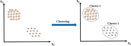
Clustering is an unsupervised machine-learning technique that classifies data points having similar properties into groups. Figure 3 shows an example of clustering where the data is composed of two clusters. Once the clustering algorithm identifies all the clusters, a selection of anomalies can be made by searching for clusters with few members. This class of algorithms has an advantage in that no prior information is assumed regarding the size of anomaly.

Figure 3. An illustration of clustering data points that belong to different groups.

Carlotto (2005) proposed a k-means cluster-based algorithm to detect the man-made targets in the imagery. The cluster-based algorithm uses a different approach as compared to the RX detector. Unlike the RX detector, the Cluster-based algorithm does not use a sliding window, instead, it uses clusters to calculate the statistics of background. The pixels of the background can be modeled as the normal distribution within a cluster around the average values whereas the anomaly pixels significantly differ from the cluster distribution. The algorithm involves an iterative process and is repeated until it converges. This technique can detect the target of any shape or size. However, one of the limitations of this technique is to define the number of clusters and another one is that the background cannot be modeled as a multivariate Gaussian model. Hytla et al. (2009) presented an extension of the cluster-based algorithm (Carlotto 2005) referred to as a fuzzy cluster-based algorithm. Fuzzy cluster tries to find soft clusters in which any data point may belong to more than one clusters. The centroids are calculated by using the mean and covariance of the background statistics. Anomalies are determined based on the membership function. This method is more flexible than cluster-based anomaly detection.

Most of the window-based detectors may contain pixels with lower spectral correlation in the local window which reduces the accuracy of the detectors. Tu et al. (2019) proposed a spatial density background purification-based technique to extract the pure background. First, a dual window density clustering approach is used to estimate the local density of the pixels. The densities are sorted and the highest densities are selected to get the pure background pixels while removing the dissimilar pixels. Finally, a collaborative representation detector (Li and Du 2015) is applied to get the anomalies with better accuracy. This technique is computationally expensive.

Tu et al. (2020b) presented intrinsic image decomposition for the first time in hyperspectral data. In this article, Retinex-Dual Window Density (R-DWD) is proposed which consists of rank intrinsic image decomposition (RIID) (Huang et al. 2018) and Dual Window Density (DWD)-based detector. The RIID is an improved version of low RIID. Its goal is to extract the reflectance component (differentiating easily between different materials) and the shading component has been eliminated. Dual window density (DWD) is proposed for the reflectance component, which relies on density peak clustering that avoids the Gaussian assumption of background distribution in hyperspectral images while improving the statistics of background. The DWD identifies anomalies of various sizes and properly determines their shape. One of the limitations of this method is parameter settings such as window size, the parameter of weight function and cut-off distance. Some of the vital information also gets removed while eliminating the shading component.

Tu et al. (2020a) proposed an algorithm based on peak density clustering to avoid the assumption of Gaussian distribution to model complete background and contamination caused by anomalies. These were two aspects affecting the detection efficiency. To overcome these limitations, the proposed method first splits the HSI image into a suitable number of local windows. Second, for each pixel of a window, it acquires the density score. In the end, anomalies are determined based on the obtained density map by adding the local density score of all local windows. Some false alarms are still produced by the proposed method, moreover, setting the parameters for various datasets is not constant in this algorithm.

3.6. Low-rank-based techniques

Low-rank-based algorithms that divide a matrix into a sum of low-rank matrix and a sparse outlier matrix have recently drawn considerable attention in the signal processing community (Candès et al. 2011). For anomaly detection, the HSI data cube can be a sum of low-rank background and a sparse anomaly matrix (Sun et al. 2014; Xu et al. 2016). Therefore, the data matrix is decomposed into two components, low-rank and sparse matrix (Y.-X. Wang et al. 2016) as demonstrated in Figure 4.

Figure 4. An illustration of the low-rank decomposition of a matrix.

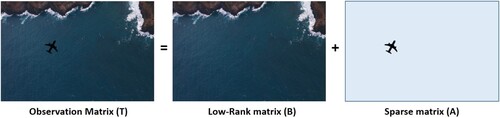
Denoting the HSI data cube as $\hat{\mathit{T}}$, the low-rank techniques decompose the data as (14) $\hat{\mathit{T}}=\hat{\mathit{B}}+\hat{\mathit{A}}.$(14) where $\hat{\mathit{B}}$ is a low-rank matrix that represents background components and $\hat{\mathit{A}}$ is a sparse matrix that contains few nonzero entries that relate to the anomalies. The decomposition in (14) can be obtained using a number of different algorithms proposed in the literature, such as Robust PCA (Candès et al. 2011).

Shuangjiang Li et al. (2015) presented an anomaly detector based on low-rank tensor decomposition. First, robust PCA is applied to separate the low-rank tensor from the sparse tensor. The low-rank tensor contains the background and anomalies, whereas the sparse tensor contains the outliers. Tucker decomposition (Kolda and Bader 2009) is applied to further break down the low-rank tensor to obtain the core tensor which includes distinct spectral signatures. Finally, an unmixing technique is used to detect the anomalies in the hyperspectral image.

Xu et al. (2016) proposed a low-rank and sparse representation-based (LRASR) technique, which separates the background and anomaly pixels. The algorithm is based on the supposition that the background and anomalies have low-rank and sparse properties respectively. A background dictionary can approximately represent each pixel in the background and a low-rank matrix is formed by the representation coefficients of all pixels, which is used to model the background component. Therefore, the background information in the low-rank matrix has low-rank properties. In this way, all pixels are characterized by a global point of view. A sparsity-inducing regularization concept is added to the representation coefficients to better describe each pixel’s local representation. In addition, to form a more robust and discriminatory dictionary, a dictionary construction technique is used. Then the anomalies are determined by the residual matrix response. One of the advantages of the proposed algorithm is that it incorporates the HSI’s global and local structure. The proposed technique is computationally expensive, and another limitation is that both anomaly and noise pixels have similar sparse characteristics. Therefore, it is exceedingly difficult to distinguish the anomaly and noise pixels.

Qu et al. (2018) presented a technique that depends on spectral unmixing and low-rank decomposition. Instead of using original data, it uses the abundance vectors obtained from the spectral unmixing algorithm as it helps remove the noise pixels. These abundance vectors have distinct features and the anomaly’s pixels can be detected easily. As the pixels of the background are highly correlated and anomaly’s pixels are sparse, therefore, a dictionary is constructed using mean shift clustering to increase the discriminative power of the technique. The constructed dictionary is based on the low-rank decomposition method. This method causes the residual matrix to remain sparse whereas the coefficients of the dictionary remain low-rank. Anomalies are determined by adding the column of the residual matrix.

Zhuang et al. (2021) proposed a hybrid denoising and anomaly detection framework which assumes that the dataset contains small number of outliers in unknown positions. The proposed anomaly detection algorithm is modeled as an optimization problem with the objective to maximize the output of the estimation matrix.

Authors proposed an autonomous hyperspectral anomaly detection network (Auto-AD) where the background is reconstructed by the network and the anomalies appear as reconstruction errors (Wang et al. 2022a). The work was further extended by developing a deep low-rank-based method, called DeepLR, that combines a model-driven low-rank prior and a data-driven autoencoder for anomaly detection by considering low-rank background estimation and network training as two sub-problems (Wang et al. 2022b).

A weakly supervised low-rank representation (WSLRR) is proposed in which a weakly supervised approach is used for background learning which does not rely on prior information (Xie et al. 2021). First background pixels are extracted from input data using coarse anomaly detector. Weakly supervised model is trained on the background data obtained from the coarse anomaly detector. A low-rank representation is utilized to extract the features of anomaly and background based on their structural properties.

3.7. Representation-based techniques

The basic idea behind representation-based methods is that every pixel in the HSI data cube can be characterized in terms of its spatial neighborhood. Therefore, background pixels are assumed to be similar to neighborhood pixels whereas anomalies are not. Consider a hyperspectral image, $\hat{\mathit{Y}}$ $\in$ ${\mathbb{R}}^{d\times n}$, which can be expressed as (15) $\hat{\mathit{Y}}=\left[\mathit{x}\left(0\right),\mathit{x}\left(1\right),\mathit{x}\left(2\right),\mathit{x}\left(3\right),\dots .\mathit{x}\left(n\right)\right],$(15) where $\hat{\mathit{Y}}$ is the HSI data cube, $\mathit{x}\left(i\right)\in {\mathbb{R}}^d$ is the spectrum of the $i^{\mathrm{t}\mathrm{h}}$ pixel, $d$ is the total number of bands and $n$ is the number of pixels. The neighborhood data to test pixel $\mathit{x}\left(i\right)$ is collected using the dual window approach (Li and Du 2015). Therefore, the number of samples obtained from the difference of windows are (16) $S=w_{out}^2-w_{in}^2.$(16)

For example, if the size of the inner and outer windows is assumed to be 3 and 5 respectively, the number of samples $S$ is 16 which is compared with the test pixels as shown in Figure 5.

Figure 5. Representation-based strategy, indicating the inner and outer windows and the test pixel.

The test hypothesis for representation-based algorithms is then formed using the residual, which is represented as (17) $d_1={\Vert \mathit{x}\text{–}\sum _{i=1}^S{\alpha }_i{\mathit{y}}_i\Vert }_2^2$(17) where $d_1$ is the residual, $S$ is the number of neighborhood pixels used for representation, $\mathit{x}$ is the pixel under test that is compared with neighborhood pixels ${\mathit{y}}_i$ and $\parallel .{\parallel }_2^2$ represents the square of $L_2$-norm. If the value of $d_1$ is greater than some predefined threshold then $\mathit{x}$ is considered anomalous (Li and Du 2015).

Li and Du (2015) proposed the collaborative representation detector (CRD). The proposed detector assumes that every band of hyperspectral image contributes equally, which is not always true (Wang et al. 2020). To overcome this limitation, Wang et al. (2020) proposed a modified version of this approach, called the self-weighted collaborative representation. The technique assigns weights based on the contribution of each band. Therefore, the band selection strategy is a special case of the self-weighted approach. This strategy integrates with collaborator representation in an objective function and it iterates over the loop until the objective function converges. This technique is susceptible to variations in regularization parameters as well as to the size of the window.

Tan et al. (2019) presented a technique called ‘the local summation anomaly detection based on collaborative representation and inverse distance weight’. This technique is based on a dual window sliding approach to avoid the contamination of anomaly pixels. Inverse distance weight is used to speed up the algorithm and collaborative representation is also introduced to increase the detection of an anomaly. However, these techniques are still computationally expensive and the selection of parameters, such as constant λ (regularization parameter) and the size of inner and outer windows are not constant for different datasets.

Huyan et al. (2019) proposed a technique based on background and anomaly dictionaries to discriminate between background, anomaly and noise pixels. Anomaly detection is a matrix decomposition problem as the original hyperspectral image is divided into the anomaly, background and noise components. The anomaly and background pixel have sparse and low-rank properties; therefore, these constraints are applied in the model. By using the prior information of background and anomalies the two dictionaries are constructed. A joint sparse representation-based dictionary selection approach is used for the background dictionary, which assumes that the commonly used atoms in the overcomplete dictionary appear to be the background. Whereas the potential anomaly dictionary is constructed by using the prior hidden anomalies information. Finally, the dictionary’s atoms are selected as per anomalous level and using the residual calculated in the joint sparse representation model together with the weighted term to reduce the effect of noise and background. Parameters setting is one of the challenging tasks of this technique.

Zhao et al. (2020) proposed an algorithm to take the advantage of spatial as well as spectral information of hyperspectral images. The proposed algorithm consists of two main techniques, i.e. Fractional Fourier transform (FrFT) (Tao et al. 2019) and CRD (Li and Du 2015). First, CRD is used which does not assume any distribution for the background, unlike traditional detectors. Next FrFT is applied to get the pixel’s feature in the intermediate domain which is in between reflectance spectrum and Fourier transform information. FrFT helps reduce the noise from the background and improves discrimination between the background and anomaly pixels. Lastly, the spectral and spatial data are mixed together to get the final result. However, one of the limitations of this technique is that it requires to set the parameters, such as inner and outer window size, optimal fractional order, regularization parameter and weighting coefficient.

A random collective representation-based detector with multiple features (RCRDMF) is proposed (Feng et al. 2022). Different kinds of features like Gabor, extended multi-attribute profile and spectral features are combined and utilized for ensemble and random collaborative detector. Background detection is done faster as random background learning is involved in this framework. Results on different datasets indicate promising performance in terms of speed and accuracy.

3.8. Deep learning-based techniques

Deep learning is a type of machine learning technique that consists of several layers that are used to extract the deep features from the original data. Deep learning is further classified into supervised, unsupervised and semi-supervised learning. In supervised learning, the model is trained using labeled data, whereas in unsupervised learning the model is trained without any labels. Finally, semi-supervised learning is a hybrid approach that lies between unsupervised and supervised learning.

3.8.1. Supervised learning techniques

Li, Wu, and Du (2017) applied a supervised deep convolution neural network (CNN) for the first time on hyperspectral anomaly detection. The network consists of 16 convolutional layers. At first, the difference between pixel pairs is generated using a reference image to obtain large number of samples. Then the network is trained on these samples to extract features such that the network can easily discriminate between similar and dissimilar pixel pairs. It finds similarity between the pixel under test and its neighborhood pixels. Anomalies are detected by taking mean of these samples which is compared with a predetermined threshold. However, this technique is computationally expensive. Yousefan et al. (2022) proposed another deep CNN which consists of four convolution layers and four dense layers. First, PCA is applied to reduce the dimensionality of the hyperspectral image. After that, the network is trained on a single image to learn the similarities between the pixels to obtain a membership map using a threshold. Then object area filtering is applied on a membership map to remove the irrelevant target to obtain a binary image. The final output is the product of a membership map and the binary filtered image. The network has fewer trainable parameters and is computationally efficient. Parameters, such as window size, thresholding and several connected components need to be selected according to the application.

Rao et al. (2022b) proposed a siamese-based transferrable network for hyperspectral anomaly detection. In this work, siamese architecture is used to identify anomaly based on the similarity of a pixel with other neighboring pixels. Spectral angle constraint and adaptive clustering are added to enhance the anomaly detection. Results indicate that its performance is comparable to other state-of-the-art algorithms.

3.8.2. Unsupervised learning techniques

A limitation of the supervised learning algorithm is that the data with ground truth is not always available. Another limitation is that the data needs to be preprocessed which may affect the results. Some of these limitations can be overcome using unsupervised learning techniques.

Bati et al. (2015) proposed an unsupervised learning technique to find anomalies. The proposed technique is based on an auto-encoder which consists of encoder and decoder parts (Ng 2011). The encoder part is used to extract the features while the decoder is used for reconstruction. Then the anomalies are determined based on the reconstruction error. This technique does not have any assumptions about the background. However, selecting the encoder and decoder function, code size and learning parameters is challenging.

A similar technique has been proposed by Rao et al. (2022a) where a siamese architecture has been proposed to construct training samples with little prior information and image itself.

A common problem with some of the previous algorithms is that the background is assumed to have a multivariate Gaussian distribution, if any pixel under test differs, then it results in a false alarm. Another problem is that the anomaly pixels may get mixed with local pixels. An unsupervised network is proposed which is based on a deep belief network and adaptive weights to resolve these problems (Ma et al. 2018). For the first time, a weighted code deep belief network was used for anomaly detection which does not assume any distribution. The network is based on an autoencoder that extracts the features from the hyperspectral image. The encoder and decoder parts generate the sequence of codes and reconstruction error respectively. Finally, adaptive weights are applied to eliminate anomalous pixel contamination. Anomalies are determined based on adaptive weights which are obtained from reconstruction errors.

Zhao and Zhang (2018) suggested an unsupervised learning method based on a low-rank and sparse matrix. First, the Go decomposition approach is used to obtain the anomaly and background pixels, in which the anomalies and background have sparse and low-rank properties respectively. Then unsupervised stacked autoencoder is applied on anomaly as well as background region to extract the spectral and spatial features. These two features are combined and finally, anomalies are detected based on Mahalanobis distance. However, the optimal parameters setting is a challenging task in this algorithm.

Zhang and Cheng (2019) proposed a staked autoencoder that is based on adaptive subspace representation. The staked autoencoder consists of multiple single-layer autoencoders. Initially, inner, outer and dictionary windows are selected which are centered at pixel under consideration, to get the dictionary and local background in the image. By using stacked autoencoder the deep features between test pixel and local dictionary pixel as well as the deep characteristics of differences between local dictionary pixels and local background pixels are also obtained. Finally, the anomalies are determined based on L2-norm by staked autoencoder adaptive subspace representation. The technique is slow, moreover, appropriate selection of windows and tuning different parameters is not an easy task.

Authors propose an anomaly detection algorithm that uses a plug-and-play denoising CNN prior to finding representation coefficients and constructs a new dictionary based on clustering (Fu et al. 2021). This plug-and-play denoising CNN regularized anomaly detection (DeCNN-AD) method is tested on five different datasets with satisfactory results.

Arisoy, Nasrabadi, and Kayabol (2021) developed a technique that employs a generative adversarial network (GAN) followed by the RX detector. In hyperspectral images most of the pixels belong to the background and anomalies consist of very few pixels. Therefore, the generator learns better features from the background compared to anomalous pixels. It generates synthetic data that is close to the background. Then the original data is subtracted from this synthetic data to get the difference image to suppress the background. The mean, as well as the covariance matrix, is computed from the difference image. Finally, anomalous scores are calculated from the difference image to detect the anomalies.

One of the problems of the hyperspectral image is that it contains lot of redundant data. Another problem is that the anomalies get overwhelmed by the surrounding pixels. To overcome these two limitations, Xie et al. (2020a) proposed a methodology called ‘Spectral Adversarial Feature Learning’. It is an unsupervised learning algorithm with encoder, decoder and discriminator components. The technique consists of two main parts: the extraction of features and iterative optimization. First, the technique extracts the distinct features after the encoding component and the reconstruction error is obtained from decoding components. Then averaging fusion method is applied to distinct features and obtain comprehensive features. The response of anomalies is further improved by using a morphological attribute filter. Finally, the adaptive weighted suppression function is used to reduce the false alarm rate and this process continues until the results of detection are stable. However, this methodology is computationally expensive.

As discussed above, the hyperspectral image contains a lot of redundant data and some of the bands have lower signal-to-noise ratio. Xie et al. (2019b) presented an unsupervised learning method based on spectral constraint adversarial autoencoder to overcome these constraints. First, the hyperspectral data is preprocessed by using the distance function to improve the spectral distance between the background and anomaly pixels. Then adversarial autoencoder is used to extract the features in the hidden layer where the decoder layer gives a reconstructed error. Spectral angle mapping is used to calculate the similarity between the reconstructed and reference image to minimize the cost function. Hidden layers are individually combined by using an adaptive weighting approach. Finally, a bi-layer framework is used to preserve the anomalies while suppressing the background.

Some of the anomaly detection techniques have lower detection accuracy and higher false alarm rates. To address this issue, Taghipour and Ghassemian (2019) presented an unsupervised autoencoder to detect the anomalies. The network has five layers with three hidden units. The techniques consist of the encoder part which extracts the features in the latent space whereas the decoder is used to reconstruct the image from these features. The majority of the pixels belong to the background and anomalies have fewer pixels. Therefore, the anomaly pixels are not learned by the model during training as the reconstruction error of anomaly pixels is always higher compared to the background. One of the advantages of this technique is that it does not use the sliding dual window approach.

3.8.3. Semi-supervised learning technique

Xie et al. (2020b) proposed a semi-supervised technique called the semi-supervised background estimation model for better discrimination between background and anomaly pixels. First, PCA is used to reduce the high-dimensional hyperspectral data. Then to cluster the data, density-based spatial clustering of applications with noise (DBSCAN) is applied, as high-probability pixels belong to the background and low-probability pixels (anomalies) are rejected. Then adversarial autoencoder is used which consists of generator and discriminator components. The generator part which is an autoencoder is used to train the model on background pixels only. The discriminator part distinguishes between the real hyperspectral data and the data generated by the generator. Finally, anomalies are determined by measuring the Mahalanobis distance between the sample and background data. However, hyperparameter tuning gets intricate.

The summary of various anomaly detection categories and techniques is shown in Table 1.

Table 1. Different anomaly detection categories and techniques were used in previous studies.

Category	Techniques
Statistics-based	Global and Local RX (Reed and Yu 1990)
	Weighted-RX (Guo et al. 2014)
	DWRX (Liu and Chang 2004)
	MWAD (Liu and Chang 2013)
	RSAD (Du and Zhang 2011)
	D-RX (Liu and Han 2017)
	FrFE (Tao et al. 2019)
	TD-TSE (Sun et al. 2021)
	EIRME (Sun et al. 2022)
Subspace-based	Subspace RX (Schaum 2004)
	UNRS (Li and Du 2013)
	BJSR (J. Li et al. 2015)
	LSAD (Du et al. 2016)
	LSUNRSORAD (Tan et al. 2019)
	GoDec (Chang et al. 2021)
	OSPGoDec (Chang, Cao, and Song 2021)
Kernel-based	Kernel RX (Kwon and Nasrabadi 2005)
	SVDD (Banerjee, Burlina, and Diehl 2006)
	RNAD (Zhao, Du, and Zhang 2014)
	CKRX (Zhou et al. 2016)
	iForest (Li et al. 2019)
Filtering-based	LFRX (Guo et al. 2014)
	AED (Kang et al. 2017)
	Multiscale AED (Li et al. 2018)
	STGF (Xie et al. 2019a)
	LAD (Verdoja and Grangetto 2020)
	SPSGF (Huang, Fang, and Li 2020)
Clustering-based	CBAD (Carlotto 2005)
	FCBAD (Hytla et al. 2009)
	SDBP (Tu et al. 2019)
	R-DWD (Tu et al. 2020b)
	DPAD (Tu et al. 2020a)
Low-Rank-based	RPCA (Candès et al. 2011)
	LTDD (Shuangjiang Li et al. 2015)
	LRASR (Xu et al. 2016)
	ADLR (Qu et al. 2018)
	RhyDe (Zhuang et al. 2021)
	Auto-AD (Wang et al. 2022a)
	DeepLR (Wang et al. 2022b)
	WSLRR (Xie et al. 2021)
Representation-based	CRD (Li and Du 2015)
	PAB-DC (Huyan et al. 2019)
	LSAD-CR-IDW (Tan et al. 2019)
	SWCRD (Wang et al. 2020)
	SSFrFTCRD (Zhao et al. 2020)
	RCRDMF (Feng et al. 2022)
Deep Learning-Based	CNND (Li, Wu, and Du 2017)
	TDLAD (Yousefan et al. 2022)
	TSN-HAD (Rao et al. 2022b)
	AE (Bati et al. 2015)
	STTD (Rao et al. 2022a)
	DBN (Ma et al. 2018)
	LRaSMD-SSSAE (Zhao and Zhang 2018)
	SAEASM (Zhang and Cheng 2019)
	SAFL (Xie et al. 2020a)
	SCAAE (Xie et al. 2019b)
	DeCNN-AD (Fu et al. 2021)
	GAN-RX (Arisoy, Nasrabadi, and Kayabol 2021)
	DAEAD (Taghipour and Ghassemian 2019)
	SBEM (Xie et al. 2020b)

The advantage and disadvantage of various anomaly detection technique are shown in Table 2.

Table 2. Advantages and disadvantages of various anomaly detection techniques.

Technique	Advantages	Disadvantages
Global RX detector	Performs well if the underlying data distribution is assumed correctly	Higher false alarm rate when background information is created using Gaussian distribution Anomaly pixels are also included in background statistics
Local RX detector	Use of a local dual window to get the local background statistics to eliminate anomalous pixels in the calculation of background	Computationally expensive Window size selection problem Model the background using a multivariate Gaussian model
Fractional Fourier Entropy RX (FrFT-RX)	Better handles the non-stationary noise	Cannot model the background with a multivariate Gaussian model
Subspace RX	It suppressed the feature of the background by using the principal component of the covariance matrix	Fails under noise
Local summation anomaly detection (LSAD)	It used spatial as well as spectral information	Uses multiple sliding windows that are time-consuming Computationally very expensive
Kernel RX	Converts a nonlinear method into a linear one in a high-dimensional feature space	Selecting a suitable kernel function is a difficult task The complexity of kernel functions often results in a lot of calculations
Isolation forest	Good accuracy in identifying outliers Good scalability	Performs poorly when there are local anomalies in the data Requires two parameters: the maximum number of trees and the number of isolated forest repeats before the algorithm is performed
Attribute & edge-preserving filtering-based detector (AED)	Utilizes local filtering operations, particularly attribute and edge preservation to detect anomalies Computationally efficient	Does not use multiscale technique to detect anomalies
Multiscale attribute & edge-preserving filtering detector (MAED)	Uses a coarse-to-fine method to detect multiscale anomalies	Computationally expensive due to multiscale and support vector machine operations
Cluster-based anomaly detector (CBAD)	Simple to use in unsupervised manners	Multivariate Gaussian models are not effective in estimating the background Number of clusters needs to be defined
Density peak clustering (DPC)	Does not require any assumptions about data distribution Eliminates the background statistics contamination by measuring deviation from the background using local density	Parameter-setting is not constant for various datasets Produces higher false alarms
Robust Principal Component Analysis (RPCA)	Works effectively for isolated pixels	Produces higher false alarm rate
Low rank and sparse representation (LRASR)	Incorporates the HSI’s global and local structure	The suggested approach requires a lot of computing Quite challenging to distinguish an anomalous pixel from a noise pixel because anomaly and noise pixels are similar sparse properties
Collaborative representation detector (CRD)	It doesn’t assume any background distribution It makes an assumption each pixel of the background can be roughly represented by the pixels around it, but the anomalous pixels cannot	Assumes that each band of hyperspectral images serves equally, which is generally incorrect Sensitive to window size
Self-weighted collaborative representation (SWCRD)	Simultaneously executes collaborative representation and automatically learns the weights for each band	Susceptible to regularization parameters as well as to the size of the window
Potential anomaly and background dictionary construction (PAB-DC)	This technique removes the impact of noise by using dictionaries to efficiently detect an anomaly	Computationally very expensive Parameters setting is also very difficult
CNN-based detection (CNND)	In CNND, input data used to train a multilayer CNN is the values that differ between adjacent pixel pairs in the reference image The trained CNN is then used in the test phase to assess changes between adjacent pixel pairs and identify anomalies	Ground truth labels are required to train a model Higher computational complexity
Autoencoder (AE)	The distribution of data is not assumed in this case. Therefore, it performs well in scenarios where Gaussian or normal distribution is not applicable	Selecting the encoder and decoder function and learning parameters are challenging tasks
Semi-supervised background estimation model (SBEM)	Exhibits very good performance as background estimation usually results in good background suppression	Hyperparameter tuning is one of the difficult problems

4. Datasets

Table 3 provides a list of publicly available datasets for hyperspectral anomaly detection along with the dataset specifications and references to previous studies using the dataset.

Table 3. General information on space-borne sensors in reviewed publications.

Datasets	Place	Sensor	Spatial resolution (m)	Wavelength (μm)	Size	References
San Diego	San Diego Airport Area	AVIRIS1	3.5	0.37–2.51	400 × 400 × 189	Huang, Fang, and Li 2020; Kang et al. 2017; Zhao, Du, and Zhang 2014; Huyan et al. 2019; Wang et al. 2020; Xu et al. 2016; Li et al. 2019; Xie et al. 2019a; Zhao et al. 2020; Du et al. 2016; Ma et al. 2018; Tan et al. 2019; Xie et al. 2020b; Zhang and Cheng 2019; Xie et al. 2020a; Zhao and Zhang 2018
ABU-Airport	Los Angeles	AVIRIS1	7.1	0.43–0.86	100 × 100 × 205	Huang, Fang, and Li 2020; Kang et al. 2017; Xie et al. 2019a; Tao et al. 2019; Tu et al. 2019; Tu et al. 2020a; Arisoy, Nasrabadi, and Kayabol 2021; Tu et al. 2020b; Xie et al. 2020b
ABU-Airport	Gulfport	AVIRIS1	3.4	0.4–2.5	100 × 100 × 191	Li et al. 2018; Tao et al. 2019; Tu et al. 2019; Arisoy, Nasrabadi, and Kayabol 2021; Xie et al. 2019a; Xie et al. 2020b; Tu et al. 2020b
ABU-Urban	Los Angeles	AVIRIS1	7.1	0.43–0.86	100 × 100 × 205	Huang, Fang, and Li 2020; Kang et al. 2017; Tu et al. 2019; Tao et al. 2019; Xie et al. 2019a; Xie et al. 2020b; Arisoy, Nasrabadi, and Kayabol 2021; Xie et al. 2020a; Tu et al. 2020a; Tu et al. 2020b
ABU-Urban	Texas Coast	AVIRIS1	17.2	0.4–2.5	100 × 100 × 204	Kang et al. 2017; Tu et al. 2019; Xie et al. 2020b; Arisoy, Nasrabadi, and Kayabol 2021; Tao et al. 2019; Xie et al. 2019a; Huyan et al. 2019; Tu et al. 2020b
ABU-Urban	Gainesville	AVIRIS1	3.5	0.4–2.5	100 × 100 × 191	Kang et al. 2017; Tao et al. 2019; Tu et al. 2019; Arisoy, Nasrabadi, and Kayabol 2021; Xie et al. 2019a; Xie et al. 2020b; Tu et al. 2020b
ABU-Beach	San Diego	AVIRIS1	7.5	0.4–2.5	100 × 100 × 193	Kang et al. 2017; Tu et al. 2019; Xie et al. 2020b; Arisoy, Nasrabadi, and Kayabol 2021; Tao et al. 2019; Xie et al. 2019a; Tu et al. 2020a; Tu et al. 2020b
ABU-Beach	Cat Island	AVIRIS1	17.2	0.4–2.5	150 × 150 × 188	Kang et al. 2017; Tao et al. 2019; Tu et al. 2019; Arisoy, Nasrabadi, and Kayabol 2021; Xie et al. 2019a; Xie et al. 2020b; Tu et al. 2020b
ABU-Beach	Bay Champagne	AVIRIS1	4.4	0.4–2.5	100 × 100 × 188	Kang et al. 2017; Tao et al. 2019; Tu et al. 2019; Arisoy, Nasrabadi, and Kayabol 2021; Xie et al. 2019a; Xie et al. 2020b; Tu et al. 2020b
ABU-Beach	Pavia	ROSIS3 -03	1.3	0.43–0.86	150 × 150 × 102	Kang et al. 2017; Tu et al. 2020b; Tao et al. 2019; Zhao et al. 2020; Arisoy, Nasrabadi, and Kayabol 2021; Xie et al. 2019a; Tu et al. 2019; Xie et al. 2020b
Urban Area	CA, USA	HYDICE	1	0.4–2.5	80 × 100 × 175	Kang et al. 2017; Li and Du 2015; Tao et al. 2019; Li et al. 2019; Xie et al. 2020b; Xie et al. 2020b
Moffett Field	CA, USA	AVIRIS	20	0.4–2.5	512 × 512 × 224	Li and Du 2015; Li, Wu, and Du 2017
Forecast scene		HYDICE	1.56	0.4–2.5	64 × 64 × 210	Li and Du 2015; Taghipour and Ghassemian 2019
Gulf of Mexico	Gulf of Mexico	AVIRIS1	7.5	0.36–2.50	280 × 180 × 258	Huang, Fang, and Li 2020
Urban area	Vegetation area	HYDICE	1	–	307 × 307 × 162	Xie et al. 2020a; Xu et al. 2016; Xie et al. 2020b
Urban area	Gainesville, FL	AVIRIS1	3.5	–	100x 100 × 191	Tu et al. 2020a
Nuance Cri	–	Nuance Cri hyperspectral	–	0.65–1.1	400 × 400 × 46	Huyan et al. 2019
World Trade Center	NewYork	AVIRIS1	–	–	200 × 200 × 224	Tao et al. 2019
SpecTIR	–	–	1	–	180 × 180 × 120	Tao et al. 2019
El Segundo	CA, USA	AVIRIS1	7.1	0.366–2.496	250 × 300 × 224	Li et al. 2019; Xie et al. 2020b
Grand Isle	Gulf Coast, LA, USA	AVIRIS1	4.4	0.366–2.496	300 × 480 × 224	Li et al. 2019
Salinas Valley (Synthetic)	California	AVIRIS1	3.7	–	512 × 217 × 224	Tan et al. 2019; Verdoja and Grangetto 2020; Li, Wu, and Du 2017; Yousefan et al. 2022
Pavia University	Italy	ROSIS	1.3	0.43–0.86	224 × 423 × 102	Tan et al. 2019; Xie et al. 2020b
HySpex	Xuzhou, China	Aircraft platform	1.5	0.415–2.508	170 × 130 × 200	Tan et al. 2019
VNIR LWIR	Rural area.	VNIR camera LWIR camera		7.8–11.5	885 × 1500 × 182 180 × 266 × 121	Bati et al. 2015
Indiana State	USA	Hyperion	–	3.57–25.76	150 × 150 × 149	Taghipour and Ghassemian 2019

These datasets are acquired from different sensors at various locations. The details of each dataset along with ground truth are explained next.

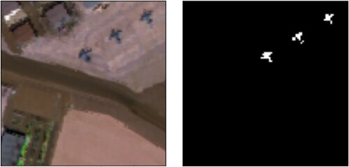
The hyperspectral data covering San Diego Airport, USA, is obtained from an Airborne Visible/Infrared Imaging Spectrometer sensor (AVIRIS-I). The image covers an area of 400 × 400 pixels and has 224 spectral bands whose wavelengths range from 0.37 to 2.51 µm. The spectral resolution is 10 nm whereas the spatial resolution is 3.5 m per pixel. The upper left part of the San Diego airport is used in the experiment which is 100 by 100 pixels. After removing the water absorption, low signal-to-noise ratio bands and poor quality bands (1–6, 33–35, 94–97,107–113, 153–166 and 221–224), 189 spectral bands are used in the experiments as shown in Figure 6.

Figure 6. A sample image of AVIRIS-I dataset (RGB) and its ground truth.

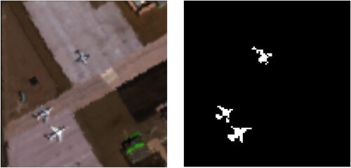
The second dataset is acquired from the AVIRIS-II sensor over San Diego CA, USA, as shown in Figure 7. The HSI image has a spatial size of 100 by 100 pixels with 189 spectral channels. The HSI has a spatial and spectral resolution of 3.5 m and 10 nm respectively. The hyperspectral image consists of grassland, airstrip and three airplanes that are considered as anomalies.

Figure 7. A sample image of AVIRIS-II dataset (RGB) and its ground truth.

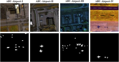
Three ABU-Airport datasets are captured from the AVIRIS sensor over the Los Angeles area and one over the Gulfport area, USA. The ABU-Airport-I, ABU-Airport-II and ABU-Airport-III cover the area of Los Angeles which is 100 by 100 pixels with 205 bands. The spectral bands range from 0.43 to 0.86 µm. The spatial resolution of a sensor is 3.4 m per pixel. Whereas the ABU-Airport-IV covers Gulfport USA. The hyperspectral image has a size of 100 by 100 pixels with 191 bands. The spatial resolution of a sensor is 7.1 m per pixel. The spectral band's range is from 0.4 to 2.5 µm. Varied sizes of airplanes are marked as anomalies as shown in Figure 8.

Figure 8. Sample images of ABU-Airport-I, ABU-Airport-II, ABU-Airport-III and ABU-Airport-IV and their ground truths.

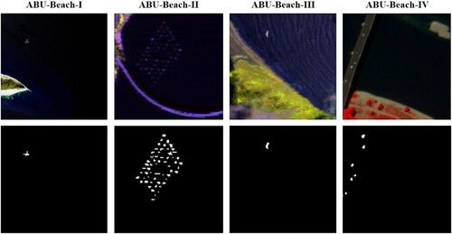
Three datasets ABU-Beach-I to III are obtained from the AVIRIS sensor whereas ABU-Beach-IV has acquired from the reflective optics system imaging spectrometer (ROSIS) sensor. ABU-Beach-I covers the area of Cat Island, Japan, and the dataset has a spatial size of 150 × 150 pixels with 188 bands and its spatial resolution is 17.2 m per pixel. ABU-Beach-II covers some of San Diego, USA. The sensor has a spatial resolution of 7.5 m per pixel. The dataset has 193 channels with a spatial size of 100 × 100 pixels. ABU-Beach-III covers the area of Bay Champagne, Vanuatu. The hyperspectral cube has a size of 100 × 100 with 188 bands and has a spatial resolution of 4.4 m per pixel. These mentioned datasets have the wavelength ranging from 0.4 to 2.5 µm. The hyperspectral image of ABU-Beach-IV is of Pavia, Italy. The hyperspectral cube has a size of 150 × 150 with 102 bands which range from 0.43 to 0.86 µm. The ROSIS-03 sensor has a spatial resolution of 1.3 m. The hyperspectral images and their ground truths are shown in Figure 9.

Figure 9. ABU-Beach-I shows images of Cat Island, Japan. ABU-Beach-II shows areas of San Diego, USA. ABU-Beach-III shows areas of Bay Champagne, Vanuatu and ABU-Beach-IV shows Pavia, Italy and their ground truths.

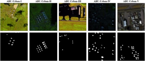
Five datasets ABU-Urban-I to V are taken from the AVIRIS sensor and each dataset has a spatial size of 100 × 100 pixels. The ABU-Urban-I and ABU-Urban-II cover the area of Texas Coast, USA, with 204 and 207 spectral bands, respectively and its spatial resolution is 17.2 m per pixel. ABU-Urban-III covers the area of Gainesville, Florida, with 191 spectral bands and its spatial resolution is 3.5 m per pixel. The ABU-Urban-I to III has spectral bands ranging from 0.4 to 2.5 µm. Whereas the ABU-Urban-IV and ABU-Urban-V datasets cover the area of Los Angeles, USA, and both have 205 spectral bands with wavelength ranging from 0.43 to 0.86 µm. Its spatial resolution is 7.1 m per pixel. The HSI datasets and their ground truths are shown in Figure 10.

Figure 10. ABU-Urban-I to V datasets acquired from the AVIRIS sensor along with their ground truths.

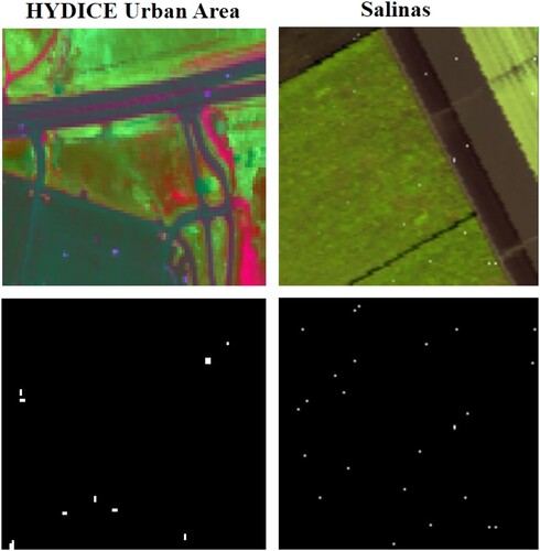
The urban dataset was taken from the Hyperspectral Digital Imagery Collection Experiment (HYDICE) sensor over the area of urban CA, USA. The scene covers an area of 80 × 120 pixels with a spatial resolution of 1 m per pixel. After removing the water absorption, 175 spectral bands were used in the experiment with wavelengths ranging from 0.4 to 2.5 µm. The image consists of roads and vegetation areas where cars and roofs are considered as anomalies as shown in Figure 11. The Salinas dataset was collected from the AVIRIS sensor over the area of Salinas Valley, CA, USA. The entire scene covers an area of 512 × 217 and has 224 spectral bands. The upper left part of the Salinas is used which is 100 × 100 pixels. After removing the water absorption and low atmospheric bands (108–112, 154–167 and 224), 220 spectral bands with a spatial resolution of 3.7 m per pixel are included. Buildings are implanted in the HSI image and are marked as anomalies as in Figure 11.

Figure 11. Urban dataset and Salinas dataset along with their ground truths.

5. Results and discussion for anomaly detection

In this section, we present our simulation results for comparing different anomaly detection techniques. The set of techniques evaluated from Statistics-based category is RX detector (Reed and Yu 1990), local RX (Reed and Yu 1990), Derivative RX (D-RX) (Liu and Han 2017), Discrete Wavelet Transform RX (DWT-RX) (Tang, Lu, and Yuan 2015; Tao et al. 2019), Random Selection-based Anomaly Detector (RSAD) (Du and Zhang 2011) and Fractional Fourier Entropy (FrFE) (Tao et al. 2019). The set of techniques evaluated from Subspace-based category is Complementary Subspace Detector (CSD) (Schaum 2004), Unsupervised Nearest Regularized Subspace (UNRS) (Li and Du 2013) and Local Summation Unsupervised Nearest Regularized Subspace with an Outlier Removal Anomaly Detector (LSUNRSORAD) (Tan et al. 2019). The set of techniques evaluated from the Filtering-based category is Attribute and Edge-preserving filtering-based Detection (AED) (Kang et al. 2017), Laplacian Anomaly Detector (LAD) using Cauchy distance (Verdoja and Grangetto 2020), LAD using Cauchy distance and spatial variant (Verdoja and Grangetto 2020), LAD using partial correlation (Verdoja and Grangetto 2020) and LAD using partial correlation and spatial variant methods (Verdoja and Grangetto 2020). The set of techniques evaluated from the Clustering-based category is Cluster-based Anomaly Detector (CBAD) (Carlotto 2005) and Fuzzy Cluster-based Anomaly Detector (FCBAD) (Hytla et al. 2009). The set of techniques evaluated from the Representation-based category is Collaborative Representation-based Detector (CRD) (Li and Du 2015) and local summation anomaly detection-based on collaborative representation and inverse distance weight (LSAD-CR-IDW) (Tan et al. 2019). The techniques evaluated from Kernel-based and Low-rank-based categories are Kernel Isolation Forest Detector (KIFD) (Li et al. 2019), Low-Rank and Sparse Representation (LRASR) (Xu et al. 2016) and CNN-based detection (CNND) (Li, Wu, and Du 2017) respectively. The optimal parameters of each detector are selected to achieve the best results. The summary of results achieved for all the simulated techniques is given in Table 1.

5.1. Evaluation metrics

Different evaluation metrics are used in the literature to measure the performance of anomaly detectors. The most commonly used metrics are receiver operating characteristics (ROC) curve (Bradley 1997; Fawcett 2006) and area under the ROC curve (AUC) (Bradley 1997; Faraggi and Reiser 2002), whereas standard spatial overlap index (SOI) is also used. The ROC curve is a graph representation for binary classification problems. The probability curve that plots the true positive rate (TPR) versus false positive rate (FPR). Whereas the TPR and FPR are the proportion of correctly and incorrectly classified data respectively. AUC computes the area under the ROC curve. It ranges from 0 to 1, where AUC = 1 implies that the algorithm can correctly distinguish between the two classes for all instances and AUC = 0 implies that the algorithm incorrectly predicts all the classes, which indicates the lowest measure of separability between the two classes. SOI is also referred to as Dice Similarly Coefficient (Zou et al. 2004) and is used to measure the similarity between two binary images (resultant image and ground truth in case of anomaly detection). SOI also ranges from 0 to 1, where SOI = 0 indicates no spatial overlap, and SOI = 1 indicates a complete overlap between resultant and ground truth images.

5.2. ROC curve for (PD, PF)

This ROC curve is a commonly used metric to analyze the performance of anomaly detection algorithms. The detection accuracy is mostly determined by the area under the ROC curve (AUC). Greater area indicates a higher probability of anomaly detection and lower false alarm rate, therefore, a higher AUC for (PD, PF) curve is preferred. However, this curve does not describe all the performance aspects of the algorithm as there is no information about the detection threshold. Therefore, other ROC curves (Chang 2021) are also used for evaluation that are discussed below.

5.3. ROC curve for (PD, tau)

This curve provides information about the algorithm's anomaly detection performance for different threshold values. This is also referred to as target detectability. Greater AUC for (PD, tau) curve indicates higher target detectability, hence it is desirable (Chang 2021).

5.4. ROC curve for (PF, tau)

This curve helps evaluate the background suppressibility of the anomaly detection algorithms. This curve gives information about the false alarm rate for different thresholds. The lower the area under this curve, the better the detector's performance so a lower area under curve $\mathrm{A}\mathrm{U}{\mathrm{C}}_{\mathrm{P}\mathrm{F},\mathrm{t}\mathrm{a}\mathrm{u}}$ curve is desirable (Chang 2021).

5.5. Background suppressibility

Background suppressibility (BS) is an evaluation metric that combines 2D ROC curves of (PD, PF) and (PF, tau). Its higher value is desirable. BS is given by (18) $\mathrm{B}\mathrm{S}=\mathrm{A}\mathrm{U}{\mathrm{C}}_{\mathrm{P}\mathrm{D},\mathrm{P}\mathrm{F}}-\mathrm{A}\mathrm{U}{\mathrm{C}}_{\mathrm{P}\mathrm{F},\mathrm{t}\mathrm{a}\mathrm{u}}$(18) The AUC for (PD, tau) and (PF, tau) are combined to create this metric. This matric is important required since the probabilities of detection and false alarm are usually inversely related. ODP indicates the effectiveness of the detector when PD and PF use the same threshold for their joint performance. This measure can be interpreted as the measure of anomaly detection as well as background detection. It is similar to the Overall Accuracy (OA) measure in classification and Medical Diagnosis Probability (MDP) that is used in medical imagery. Higher value of ODP is desirable (Chang 2021). (19) $\mathrm{O}\mathrm{D}\mathrm{P}=\mathrm{A}\mathrm{U}{\mathrm{C}}_{\mathrm{P}\mathrm{D},\mathrm{P}\mathrm{F}}+\mathrm{A}\mathrm{U}{\mathrm{C}}_{\mathrm{P}\mathrm{D},\mathrm{t}\mathrm{a}\mathrm{u}}-\mathrm{A}\mathrm{U}{\mathrm{C}}_{\mathrm{P}\mathrm{F},\mathrm{t}\mathrm{a}\mathrm{u}}$(19)

5.6. Signal to noise probability ratio (SNPR)

Signal to Noise Probability Ratio (SNPR) (Chang 2021) is a very effective evaluation metric for anomaly detection as its value is inversely proportional to the false alarm probability. Therefore, it is sensitive to false alarms. SNPR is inspired from SNR that is commonly used in the wireless domain as well as in signal and systems. The SNPR in given by (20) $\mathrm{S}\mathrm{N}\mathrm{P}\mathrm{R}={\displaystyle \frac{\mathrm{A}\mathrm{U}{\mathrm{C}}_{\mathrm{P}\mathrm{D},\mathrm{t}\mathrm{a}\mathrm{u}}}{\mathrm{A}\mathrm{U}{\mathrm{C}}_{\mathrm{P}\mathrm{F},\mathrm{t}\mathrm{a}\mathrm{u}}}}$(20)

5.7. Parameter setting

First, the traditional Global RX detector is applied to different datasets. The RX detector considers the background as a multivariate Gaussian model which is not a good assumption in practice as the background may be complex and may not follow a Gaussian distribution. Another limitation is that the mean and covariance matrix calculated from a contaminated background also affects the performance of the detector.

The Local RX (LRX) has two parameters, i.e. inner and outer windows. The detector is sensitive to window sizes. The inner window size must be greater than or equal to the size of an anomaly. Therefore, the inner window size varies from 3 to 19 pixels whereas the outer window size ranges from 15 to 29 pixels. The optimal window sizes are selected for each dataset based on the best AUC achieved. The LRX is computationally expensive because it needs to calculate and invert a large covariance matrix and the contamination of anomalies in the inner window also affects the results. The computation time also increases when the difference between the inner and outer windows increases.

Algorithms, such as spectral derivative and discrete wavelet transform, used for feature extraction, have been used in previous studies. In Derivative RX (D-RX), the only parameter is the step size of the derivative, which is 4 for all the datasets (Tao et al. 2019). Whereas in discrete wavelet transform RX (DWT-RX), single-level Haar decomposition is used for anomaly detection.

For the CSD detector, background and anomalies are projected to some other subspace to increase the separation between them. The number of larger eigenvalues is small and it represents the background. The number of background subspace is equivilant to the classes of background. The number of subspaces of background can be determined using an endmember extraction algorithm such as HySime. The optimal values for subspace are selected for each dataset based on the best value of AUC achieved.

The Random Selection Anomaly detector is based on statistical methods and requires three parameters, i.e. number of randomly selected blocks $M$, number of random selections $L$ and the percentile $\alpha$. The number of random blocks should be greater than four times the number of bands $B,$ so that $4M>B$. The number of random selections is 40 and the percentile values vary from 0.001 to 100 with a step size of 10 (Verdoja and Grangetto 2020).

The representation-based algorithm (CRD) has three parameters: inner and outer window sizes and the regularization parameter ${\lambda }_a$. The effect of each parameter is analyzed in this survey. The CRD performance is insensitive to the regularization parameter but ${\lambda }_a={10}^{-6}$ in the original work. The inner and outer windows are selected based on the size of the anomalies. The window sizes have an enormous impact on results. Therefore, the inner window size varies from 3 to 21 pixels whereas the outer window size ranges from 5 to 23 pixels.

The subspace-based detector, UNRS gives promising results on different datasets. The UNRS has three parameters: window sizes (inner and outer windows) and regularization parameter $\lambda$. The detector is insensitive to $\lambda$ which is kept fixed at 0.01. The inner and outer windows vary from 3 to 21 pixels and 5 to 23 pixels respectively. When the difference between inner and outer windows increases then the number of samples also increases, i.e. $S=w_{out}^2-w_{in}^2$, which in turn increases the computation cost.

The cluster-based algorithms, such as CBAD and FCBAD, have better performance in terms of execution time. The number of clusters $K$ should be predefined in clustering algorithms. The number of clusters is varied from 2 to 15 to analyze the effect of clusters on AUC values. The AUC mostly increases when the number of clusters increases in FCBAD, whereas in CBAD it is the opposite. When the number of clusters increases so does computation time.

The Local Summation Anomaly Detection (LSAD) has a single parameter, i.e. the inner window. This algorithm uses a smaller window than the local RX detector to obtain better results due to its summarization of multiple local distribution feature statistics (Du et al. 2016). The inner window size varies from 3 to 9 pixels. The computation time increase with an increase in the window size because it needs to invert a covariance matrix. LSAD uses a single window that causes a high false alarm rate and it may include contamination. As the window size increases, the cost of inversion of the matrix also increases.

Local Summation Unsupervised Nearest Regularized Subspace with an Outlier Removal Anomaly Detector (LSUNRSORAD) and Local Summation Anomaly Detection based on Collaborative Representation and Inverse Distance Weight (LSAD-CR-IDW) perform better in terms of AUC. Both algorithms have three parameters: inner and outer windows and regularization parameter $\lambda$. The inner and outer windows vary from 3 to 9 pixels and 5 to 11 pixels respectively. Whereas the regularization parameter is 100 for all the datasets. LSUNRSORAD is based on the idea that the central pixel can be represented by neighborhood pixels and LSAD-CR-IDW uses the concept of surrounding pixels which is followed by collaborative representation and inverse weight matrix. If the inner window size is small and the outer window size is large, then the computation time for both increases significantly.

The Low Rank and Sparse Representation (LRASR) has three parameters that need to be tuned according to each dataset. For dictionary construction, the number of clusters $K$ and the number of pixels in the cluster $P$ are selected. The value of $K$ is 15 and the value of $P$ varies from 20 to 50 for various datasets. The optimal value of the regularization parameter $\lambda$ is selected based on the best AUC achieved. For different datasets, the regularization parameter is either 0.1 or 0.01 to achieve the optimal detection performance.

Filtering-based technique, i.e. attribute and edge-preserving filter has drawn much attention due to its good results on most of the datasets and requires less computation time compared to other anomaly detectors. First, PCA is applied to higher dimensional data to reduce the number of dimensions, represented by $M$, which is set as 3, as also mentioned in the original work. Then attribute filter with a threshold value $K$ is set according to the size of anomaly. The values of $K$ used in our simulation are 5, 25 and 64 for different datasets. The domain transform recursive filter has two parameters ${\sigma }_s$ and ${\sigma }_r$ which controls the smoothness of the output. The value of ${\sigma }_s$ is 5 and those of ${\sigma }_r$ are either 0.5 or 1 for different datasets to achieve the best detection results.

The kernel isolation forest has promising results in detecting anomalies. First, the kernel PCA is used to transform the data to a higher-dimensional space. The number of principal components, $K$, is 300 and the Gaussian function is used as a kernel. The isolation forest has two input parameters, i.e. randomly selected pixels $M$ and the number of trees $q$. The value of $M$ is selected based on 3% of rows $\times$ columns of hyperspectral image and $q$ is set to 1000 for all the datasets.

Four different variants were used in our simulations, i.e. Laplacian Anomaly Detector (LAD) using Cauchy distance (Lc), LAD using Cauchy distance and spatial variant (Lcs), LAD using partial correlation (Lq) and LAD using partial correlation and spatial variant (Lqs) methods. The performance of LAD using Lq and Lc is quite similar. As Lc creates a model of the background without the use of matrix inversions, making it both faster and more accurate. The performance of the statistic-based technique, i.e. Fractional Fourier Entropy (FrFE) is also evaluated in this study. It has a parameter of fractional order $p$ which ranges from 0 to 1 with an interval of 0.1 for different datasets. However, the FrFE algorithm is more susceptible to the size of anomalies.

Finally, the CNND model which is a supervised learning technique consists of sixteen convolutional layers. While training the algorithm, the weights are learned automatically. Adam optimizer and binary cross-entropy loss are used. The CNND architecture has multiple other important parameters, e.g. learning rate is set to 0.001, the number of epochs is 50, and batch size is 128. The inner and outer windows are 3 and 5 for all datasets respectively. For training, the AVIRIS dataset’s Salinas scene is used, which was acquired by the Airborne AVIRIS sensor above Salinas Valley, California. It has a high spatial resolution of 3.7 m per pixel. The image contains 512 lines by 217 samples and 224 bands with 16 categories in the training image. Pixel pairs of similar and dissimilar categories are built and used to train the network. Other datasets are used for testing.

The program of each selected detection algorithm is publicly available. Links to individual programs are available at: https://github.com/NomanShahRaza/hyperspectral_anomaly_detection_algorithms.

5.8. Performance comparison

Tables 4–6 summarize the AUC results of different anomaly detectors on different datasets used in this study. The highest AUC values of each dataset are highlighted in bold. Among all detectors, AED exhibits the highest AUC of 0.9971, 0.9923, 0.9936, 0.9756, 0.9953 and 0.9976 on AVIRIS-I, ABU airport I, ABU airport II, ABU airport III, ABU airport IV, ABU Urban II datasets respectively. KIFD has the highest AUC of 0.9917 and 0.9896 on AVIRIS-II and ABU-Beach-II datasets respectively. LRX gives the highest AUC of 0.9989 and 1 on ABU-Beach-I and ABU-Beach-III datasets respectively. LSUNRSORAD exhibits the highest AUC of 0.99394, 0.99621 and 0.99078 on ABU-Beach-IV, ABU-Urban-IV and ABU-Urban-V datasets respectively. LSAD-CR-IDW, FCBAD, UNRS and LSAD shows the highest AUC of 0.99078, 0.9994, 0.99856 and 1 on ABU-Beach- I, ABU-Urban-II, HYDICE Urban Area and Salinas respectively.

Table 4. AUC scores obtained on different datasets by the RX, LRX, D-RX, DWT-RX, CBAD, FCBAD and AED anomaly detectors.

Datasets	RX	LRX	D-RX	DWT-RX	CBAD	FCBAD	AED
AVIRIS-I	0.9091	0.9881	0.9662	0.9562	0.9487	0.5148	0.9971
AVIRIS-II	0.9403	0.9598	0.9786	0.9605	0.9597	0.9883	0.9850
ABU-Airport-1	0.8221	0.8988	0.8456	0.8645	0.8686	0.9091	0.9923
ABU-Airport-2	0.8404	0.9549	0.8839	0.9077	0.9127	0.9525	0.9936
ABU-Airport-3	0.9288	0.9334	0.9157	0.9317	0.8396	0.9410	0.9756
ABU-Airport-4	0.9526	0.9811	0.9672	0.9757	0.9430	0.9821	0.9953
ABU-Beach-1	0.9807	0.9989	0.9818	0.9752	0.9887	0.9838	0.9974
ABU-Beach-2	0.9106	0.9334	0.9099	0.9183	0.9615	0.9247	0.955
ABU-Beach-3	0.9998	1	0.9998	0.9998	0.9998	0.9823	0.9997
ABU-Beach-4	0.9538	0.9790	0.9594	0.966	0.8813	0.9701	0.9799
ABU-Urban-1	0.9907	0.9604	0.9918	0.9910	0.741	0.9920	0.9981
ABU-Urban-2	0.9946	0.9542	0.9948	0.9945	0.9900	0.9994	0.8335
ABU-Urban-3	0.9513	0.9821	0.9501	0.9634	0.9640	0.9386	0.9976
ABU-Urban-4	0.9887	0.9835	0.9815	0.9850	0.6165	0.9914	0.9912
ABU-Urban-5	0.9692	0.9541	0.9617	0.9663	0.7684	0.9603	0.9845
HYDICE Urban Area	0.9857	0.9971	0.9873	0.9898	0.9924	0.9226	0.9951
Salinas	0.80732	0.9916	0.9658	0.8966	0.7665	0.9844	0.9634

Note: The highest AUC values of each dataset are highlighted in bold.

Table 5. AUC scores obtained on different datasets by the KIFD, CRD, FrFE, CSD, LSAD, UNRS, RSAD and LRASR anomaly detectors.

Datasets	KIFD	CRD	FrFE	CSD	LSAD	UNRS	RSAD	LRASR
AVIRIS-I	0.9844	0.9790	0.5252	0.9398	0.94956	0.99346	0.97256	0.9694
AVIRIS-II	0.9917	0.9412	0.9793	0.9096	0.94749	0.96773	0.89896	0.9515
ABU-Airport-1	0.9397	0.9643	0.8825	0.8145	0.93231	0.95578	0.83703	0.8647
ABU-Airport-2	0.9794	0.9653	0.7476	0.8357	0.91776	0.98096	0.83918	0.9029
ABU-Airport-3	0.9623	0.9312	0.9415	0.9245	0.91931	0.95117	0.90346	0.8926
ABU-Airport-4	0.9763	0.9630	0.9756	0.9515	0.95713	0.98602	0.9498	0.9465
ABU-Beach-1	0.9902	0.9974	0.9796	0.9848	0.95993	0.99799	0.98148	0.9719
ABU-Beach-2	0.9896	0.9803	0.9315	0.9111	0.96358	0.98292	0.94123	0.9566
ABU-Beach-3	0.9983	0.9999	0.9996	0.9999	0.99961	0.99999	0.92505	0.9995
ABU-Beach-4	0.8275	0.9396	0.9061	0.9556	0.90535	0.96557	0.81175	0.9644
ABU-Urban-1	0.9235	0.9961	0.9891	0.9905	0.97597	0.99778	0.91363	0.9342
ABU-Urban-2	0.8605	0.9460	0.9950	0.9950	0.88181	0.97348	0.82366	0.9712
ABU-Urban-3	0.9909	0.9739	0.9626	0.9571	0.98686	0.97131	0.7756	0.9461
ABU-Urban-4	0.9788	0.9855	0.9796	0.9890	0.92811	0.96179	0.92023	0.9537
ABU-Urban-5	0.9857	0.9436	0.9717	0.9702	0.91833	0.9522	0.93455	0.9407
HYDICE Urban Area	0.9966	0.9971	0.9901	0.9873	0.99522	0.99856	0.90205	0.9919
Salinas	0.9948	0.9271	0.9147	0.9873	1	0.9996	0.96156	0.9681

Note: The highest AUC values of each dataset are highlighted in bold.

Table 6. AUC scores obtained on different datasets by the LSUNRSORAD, LSAD-CR-IDW, Lc, Lcs, Lq, Lqs and CNND anomaly detectors.

Datasets	LSUNRSORAD	LSAD-CR-IDW	Lc	Lcs	Lq	Lqs	CNND
AVIRIS-I	0.9895	0.98719	0.98202	0.98779	0.98034	0.9836	0.91459
AVIRIS-II	0.98939	0.98631	0.98554	0.9878	0.9878	0.98295	0.83629
ABU-Airport-1	0.97984	0.98188	0.64488	0.7292	0.64161	0.81267	0.62903
ABU-Airport-2	0.97123	0.97713	0.76175	0.85238	0.75925	0.90051	0.59098
ABU-Airport-3	0.96615	0.97438	0.90117	0.93355	0.90772	0.94215	0.74181
ABU-Airport-4	0.98162	0.99032	0.80761	0.85601	0.78777	0.88044	0.96041
ABU-Beach-1	0.99063	0.99467	0.92025	0.9654	0.91858	0.97023	0.98528
ABU-Beach-2	0.9633	0.97953	0.65195	0.73873	0.68687	0.85332	0.87947
ABU-Beach-3	0.99911	0.99997	0.8545	0.91154	0.85454	0.96929	0.96327
ABU-Beach-4	0.99394	0.98286	0.8444	0.91137	0.85003	0.96125	-
ABU-Urban-1	0.99846	0.9985	0.98533	0.98796	0.98422	0.99091	0.88774
ABU-Urban-2	0.99553	0.98896	0.99898	0.99561	0.99914	0.99511	0.74481
ABU-Urban-3	0.99456	0.99209	0.95768	0.94864	0.92302	0.95905	0.93610
ABU-Urban-4	0.99621	0.99198	0.99284	0.99249	0.99361	0.99098	0.75167
ABU-Urban-5	0.99078	0.98905	0.95002	0.94754	0.95062	0.95386	0.90203
HYDICE Urban Area	0.98028	0.99443	0.77253	0.77416	0.80057	0.86262	0.76847
Salinas	0.99925	0.99988	0.89531	0.82605	0.90175	0.92045	0.97928

Note: The highest AUC values of each dataset are highlighted in bold.

Table 7 shows the mean and median of AUC computed for each algorithm on all the considered hyperspectral datasets. Green, yellow and blue colors represent the best, second-best and third-best mean and median AUC values among all the considered detectors. While considering the mean AUC values, LSAD-CR-IDW performs the best, whereas considering median AUC values, AED outperforms all other algorithms. However, while considering both the mean and median AUC, AED, LSUNRSORAD, LSAD-CR-IDW and UNRS appear to have a similar performance which is significantly better than the remaining algorithms.

Table 7. The mean and median AUC values of all algorithms on all datasets.

Note: Green, yellow and blue colors represent the best, second-best and third-best mean and median AUC values among all the considered detectors.

A comparison of anomaly detection in terms of computation time on two different hyperspectral datasets is presented in Table 8. The two datasets are selected based on the size of the anomalies. AVIRIS-I has larger-sized anomalies, whereas, HYDICE has relatively smaller-sized anomalies. All results were obtained using the same computer with an Intel Core i7-9700 processor, 16GB RAM, using MATLAB 2018b and Python 3.8.5.

Table 8. Computation time (seconds) of various techniques on the AVIRIS-I and HYDICE datasets.

Dataset	AVIRIS-I
Technique	AUC	Time (sec)	Technique	AUC	Time (sec)
RX	0.9091	0.07	CSD	0.9398	0.1595
LRX	0.9881	9.325	LSAD	0.94956	1179.3037
D-RX	0.9662	0.0976	UNRS	0.99346	7.3214
DWT-RX	0.9562	4.3859	RSAD	0.97256	18.9412
CBAD	0.9487	0.4787	LRASR	0.9694	69.2397
FCBAD	0.9796	13.8791	LSUNRSORAD	0.9895	1006.827
FrFE	0.5252	12.0279	LSAD-CR-IDW	0.98719	1751.783
AED	0.9971	0.3095	Lc	0.98202	0.0386
KIFD	0.9844	73.4854	Lcs	0.98779	0.6574
CRD	0.9790	6.9982	Lq	0.98034	0.1135
Lqs	0.9836	0.751	CNND	0.91459	33.5128
Dataset	HYDICE Urban Area
Technique	AUC	Time (sec)	Technique	AUC	Time (sec)
RX	0.9857	0.0555	CSD	0.9873	0.1306
LRX	0.9971	9.325	LSAD	0.99522	896.8668
D-RX	0.9873	0.08311	UNRS	0.99856	2.2802
DWT-RX	0.9898	3.17247	RSAD	0.90205	17.26
CBAD	0.9924	0.33853	LRASR	0.9919	57.6368
FCBAD	0.9226	15.7163	LSUNRSORAD	0.98028	66.7
FrFE	0.9901	8.99327	LSAD-CR-IDW	0.99443	264.3996
AED	0.9951	2.07043	Lc	0.77253	0.029248
KIFD	0.9966	47.1765	Lcs	0.77416	0.48237
CRD	0.9971	2.2754	Lq	0.80057	0.038045
Lqs	0.86262	0.54695	CNND	0.76847	18.746

The RX, D-RX, CBAD, CSD, Lc, Lcs, Ls and Lsq detectors have a computation time of less than 1 second on both datasets. Whereas CSD and AED also have computation time of less than 1 second on the AVIRIS-I dataset. AED uses dimensionality reduction techniques as a preprocessing step because of which it provides faster detection on both datasets. LRASR is based on dictionary construction which is why they require more computation time. The computation time of the deep learning technique, CNND, during testing is higher because the model consists of 16 convolutional layers. LRX, CRD, LSAD, UNRS, LSUNRSORAD, and LSAD-CR-IDW use sliding window approaches. The window sizes depend upon the size of anomalies. These algorithms have higher computation time on AVIRIS-I datasets because the size of anomalies is larger, hence it uses bigger window sizes, whereas in the HYDICE dataset the window sizes are smaller which entails less computation time. The computation time of DWT-RX, FCBAD, KIFE, FrFE and RSAD are better than some of the window-based detectors. For the AVIRIS-1 dataset, AED gives the best performance considering AUC and processing time. Whereas, for the HYDICE dataset, UNRS gives the best overall performance considering AUC and processing time.

6. Discussion

• While the overall results in Table 7 show that LSAD-CR-IDW, LSUNSORAD and AED provide the best anomaly detection performance on the considered datasets, AED provides the best combination of detection performance and computation time. Furthermore, results show that the performance of different anomaly detectors varies with the size of the anomalies. The hyperspectral datasets used in this paper have either a single or mixed anomaly of various sizes. The following insights can be extracted from the results described above. For anomalies of larger size, AED and KIFD detectors are better suited.

• In general, all detectors perform well when there is a single anomaly in the hyperspectral image. This happens as there is less background contamination in such datasets.

• When there are anomalies of different sizes in the dataset, AED and LSAD-CR-IDW give the best detection performance.

• LSAD-CR-IDW and LSUNRSORAD performed best when there are a lot of small anomalies which are randomly distributed in the dataset. On the other hand, global algorithms such as RX detector do not perform well in such scenarios because background estimate is contaminated by the anomalies.

• When there is a significant number of anomalies located close to each other, KIFD, CRD and UNRS give satisfactory results. In such datasets, the selection of window sizes for dual window algorithms becomes a challenge since selecting the wrong size results in background contamination.

• Although performance comparison shows that sliding window approaches, such as, LSUNRSORAD and LSAD-CR-IDW yield the best detection performance, in general, this performance can only be achieved if the window sizes of these algorithms are set correctly.

• In applications where no prior information is available regarding the type of anomaly in the data, global algorithms such as D-RX and DWT-RX might be better suited since they do not have any tunable parameters.

• Overall global detectors and filtering-based algorithms provide the fastest detection.

6.1. 3D ROC results and analysis

6.1.1. Experiments on ABU-Airport 3 dataset

A detailed performance analysis is done on ABU-Airport 3 dataset using 3D ROC curves. This evaluation is done for three algorithms, i.e. AED, LSADCR and LSUNRS, because these are the best three algorithms according to the median values of AUC in the previous performance analysis. Figure 12(a) shows the (PD, PF) curve, in which AED outperforms the other two algorithms as its area under the curve is highest followed by LSUNRS and LSADCR. Similar trend can be seen in Figure 12(b) that shows the ROC curve of (PD, tau). As AED has the highest area, therefore, its anomaly detectability is the highest followed by LSUNRS and AED. ROC curve of (PF, tau) shown in Figure 12(c) indicates that LSADCR has the lowest false alarm for different values of tau. In other words, its background suppression is the highest followed by LSUNRS and AED. The numeric result in Table 9 also shows similar trend. Background suppressibility (BS) of LSUNRS is the highest, whereas the overall detection probability (ODP) of AED is the highest, which indicates that AED performs best while considering detection probability and false alarm rate at a given threshold. Whereas LSUNRS has the highest SNPR, which indicates an optimum trade-off between detectability (PD, tau) and background suppressibility (Pf, tau).

Figure 12. (a)–(c) ROC curves (PD, PF), (PD, tau) and (PF, tau) for ABU-Airport 3 dataset. (d) Seperability Map.

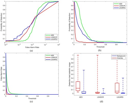
Table 9. Evaluation metrics for ABU-Airport 3 dataset.

Evaluation metrics	AED	LSADCR	LSUNRS
Area under PFPD	0.9756	0.9744	0.9661
Area under tauPD	0.1852	0.0276	0.1140
Area under tauPF	0.0225	0.0028	0.0076
BS	0.9531	0.9716	0.9585
ODP/MDP	1.1627	1.0248	1.1064
SNPR	8.231111	9.857143	15

Finally, box plot in Figure 12(d) shows that AED and LSUNRS perform better due to clearer differences between the test statistic distributions for anomaly and background. Therefore, in practical applications, setting a threshold gets easier for these two algorithms. Whereas in case of LSADCR, the separation of test statistic distributions for anomaly and background is very less, which makes it difficult to set the threshold.

6.1.2. Experiments on ABU-Urban 4 dataset

Figure 13(a) shows that in terms of ROC curve of (PD, PF), LSUNRS performs the best followed by LSADCR and AED. The curves for LSADCR and AED are very close to each other. The (PD, tau) curve indicates that AED has the highest detection probability followed by LSUNRS and LSADCR. The (PF, tau) curve indicates that LSADCR has the lowest false alarm rate followed by LSUNRS and AED. AUC results in Table 10 also indicate similar pattern. Background suppressibility of LSUNRS is the highest, whereas the overall detection probability (ODP) of AED is the highest. LSADCR exhibits the highest SNPR. The boxplot in Figure 13(d) indicates that AED has the highest separation between the anomaly and background test statistic. Overall, AED and LSADCR perform very well for this dataset.

Figure 13. (a)–(c) ROC curves (PD, PF), (PD, tau) and (PF, tau) for ABU-Urban 4 dataset. (d) Seperability Map for ABU-Urban 4 dataset.

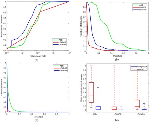
Table 10. Evaluation metrics for ABU-Urban 4 dataset.

Evaluation metrics	AED	LSADCR	LSUNRS
Area under PFPD	0.9912	0.9920	0.9962
Area under tauPD	0.3493	0.0408	0.1174
Area under tauPF	0.0307	0.0013	0.0044
BS	0.9605	0.9907	0.9918
ODP/MDP	1.3186	1.0395	1.113
SNPR	11.37785	31.38462	26.68182

6.1.3. Experiments on HYDICE Urban dataset

The ROC curve of (PD, PF) in Figure 14(a) indicates that the performance of AED and LSADCR is very good. AED crosses LSADCR in the middle. As shown in Table 11, the AUC is highest for AED followed by LSADCR and LSUNRS. The ROC curve of (PD, tau) in Figure 14(b) indicates that LSUNRS has the highest AUC, followed by AED and LSADCR. The ROC curve of (PF, tau) in Figure 14(c) indicates that LSADCR has the least false alarm rate, therefore, its area under curve is the least. Table 11 shows that the background suppressibility of LSADCR is the highest, closely followed by AED. Overall detection probability (ODP) of LSUNRS is the highest, whereas AED has the highest SNPR.

Figure 14. (a)–(c) ROC curves (PD, PF), (PD, tau) and (PF, tau) for HYDICE Urban dataset. (d) Seperability Map for HYDICE Urban dataset.

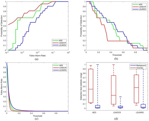
Table 11. Evaluation metrics for HYDICE Urban dataset.

Evaluation metrics	AED	LSADCR	LSUNRS
Area under PFPD	0.9951	0.9944	0.9803
Area under tauPD	0.4389	0.3494	0.4562
Area under tauPF	0.0307	0.0274	0.0430
BS	0.9644	0.967	0.9373
ODP/MDP	1.4082	1.322	1.4132
SNPR	14.29642	12.75182	10.6093

6.1.4. Experiments on AVIRIS-I dataset

The ROC curve of (PD, PF) in Figure 15(a) indicates that the performance of AED and LSADCR is very good. AED crosses LSADCR in the middle. As shown in Table 12, the AUC is highest for AED followed by LSADCR and LSUNRS. The ROC curve of (PD, tau) in Figure 15(b) indicates that LSUNRS has the highest AUC, followed by AED and LSADCR. The ROC curve of (PF, tau) in Figure 15(c) indicates that LSADCR has least false alarm rate, therefore, its area under curve is least. Table 12 shows that the background suppressibility of LSADCR is the highest, closely followed by AED. Overall detection probability (ODP) of LSUNRS is the highest, whereas AED has the highest SNPR.

Figure 15. (a)–(c) ROC curves (PD, PF), (PD, tau) and (PF, tau) for AVIRIS-I dataset. (d) Seperability Map for AVIRIS-I dataset.

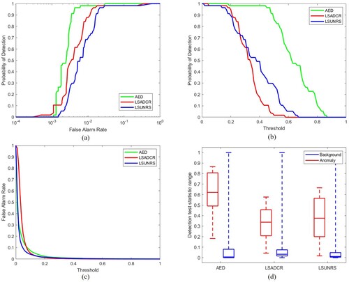
Table 12. Evaluation metrics for AVIRIS-1 dataset.

Evaluation metrics	AED	LSADCR	LSUNRS
Area under PFPD	0.9971	0.9897	0.9863
Area under tauPD	0.6411	0.3259	0.3766
Area under tauPF	0.0302	0.0432	0.0258
BS	0.9669	0.9465	0.9605
ODP/MDP	1.6109	1.2827	1.3508
SNPR	21.22848	7.543981	14.5969

6.1.5. Experiments on AVIRIS-II dataset

From Figure 16(a)–(c) it can be seen that LSUNRS performs the best in terms of ROC (PD, PF), followed by LSADCR and AED. In terms of (PD, tau), AED outperforms other algorithms. Similarly, AED has the least false alarms. Table 13 indicates that background suppressibility of LSUNRS is the highest, closely followed by AED. While considering ODP and SNPR, AED is the clear winner followed by LSUNRS. From the box-plot in Figure 16(d), it can be seen that there is separation between the distributions of test statistics of anomaly and background for all three algorithms.

Figure 16. (a)–(c) ROC curves (PD, PF), (PD, tau) and (PF, tau) for AVIRIS-II dataset. (d) Seperability Map for AVIRIS-II dataset.

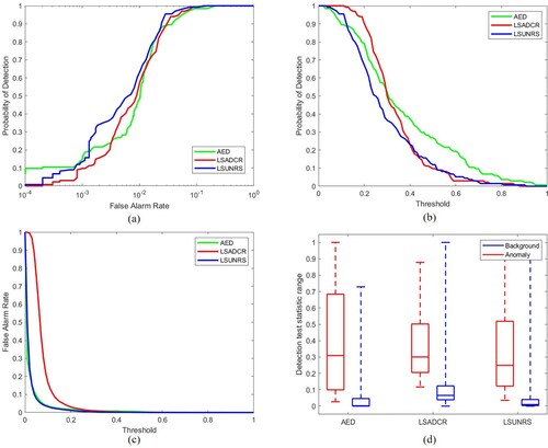
Table 13. Evaluation metrics for AVIRIS-II dataset.

Evaluation metrics	AED	LSADCR	LSUNRS
Area under PFPD	0.9846	0.9863	0.9894
Area under tauPD	0.3693	0.3361	0.2953
Area under tauPF	0.0193	0.0773	0.0207
BS	0.9653	0.909	0.9687
ODP/MDP	1.35	1.2588	1.2746
SNPR	19.13472	4.347995	14.2657

7. Dimensionality reduction of hyperspectral dataset

Dimensionality reduction is a technique to transform higher dimensional data to some lower dimension. The hyperspectral images have hundreds of bands and require enormous computation power. However, the hyperspectral image also has a significant amount of redundant data which can be minimized through dimensionality reduction, which in turn reduces the computation requirement. Dimension reduction, as mentioned in Borghys et al. (2012), Chen et al. (2014), Kåsen et al. (2008), Shen and Bassett (2002), can significantly improve the efficiency of anomaly detection in hyperspectral data. Dimensionality reduction can be accomplished using Principal Component Analysis (PCA) (Pearson 1901; Rodarmel and Shan 2002; Van Der Maaten, Postma, and den Herik 2009; Wold, Esbensen, and Geladi 1987), Independent Component Analysis (ICA) (Comon 1994; Du, Kopriva, and Szu 2006; Hyvarinen 1999; Hyvärinen and Oja 2000), Singular Value Decomposition (SVD) (Golub and Reinsch 1971; Klema and Laub 1980; Wall, Rechtsteiner, and Rocha 2003) and Factor Analysis (FA) (Lavanya and Sanjeevi 2013; Spearman 1961; Thurstone 1947; Wang and Wang 2015).

7.1. Principal component analysis

PCA is the most popular linear dimensionality reduction technique. It performs dimensionality reduction to transform the data into a linear lower subspace dimension while using an orthogonal transformation (Van Der Maaten, Postma, and den Herik 2009). It simply converts closely related variables into uncorrelated variables in a group. The primary advantage of PCA is to find similar patterns in data, thereby reducing the dimensions without losing significant information. For our simulations, we varied the number of principal components from 2 to 179 which is then followed by the RX detector. To investigate the effects of the PCA bands on anomaly detection, detailed analysis is performed. As the number of PCA bands increases, the information quality decreases and the majority of the information may only be found in the first few PCA bands. The first few PCA bands account for the bulk of the variability and the remaining bands quickly become noise. The results of the RX detector on principal components with AUC are shown in Figure 17.

Figure 17. AUC evaluation of RX detectors using PCA.

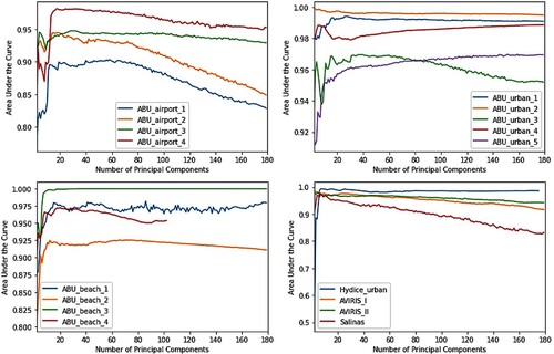
7.2. Independent component analysis

ICA is another linear transformation technique for dimensionality reduction. ICA looks for the independent factors. This technique is an extension of PCA that takes the independence of the statistics of second-order and describes the orthogonal directions. The statistically independent components are represented by this approach. As a result, the statistical dependency between its components is minimized (Comon 1994). In our simulations, the number of components of ICA is varied from 2 to 179. The results of the RX detector on the number of components with AUC are shown in Figure 18. The use of ICA as a dimensionality reduction step which is followed by the RX detector is investigated. By applying the RX detector on different components of ICA, the overall AUC increases in the reduced feature space for various datasets. As the number of component decreases, the AUC of most datasets also increases, as indicated in Figure 18.

Figure 18. AUC evaluation of RX detectors using ICA.

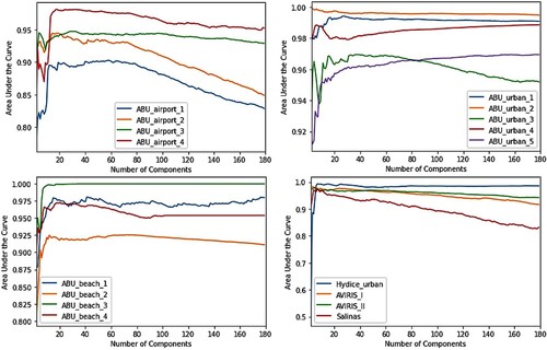
7.3. Singular value decomposition

Another commonly used dimensionality reduction technique is SVD. This technique establishes a linear function transformation to convert the parameters into independent variables. Unlike PCA, this algorithm does not center the data before measuring the singular value decomposition. Therefore, it can effectively deal with sparse matrices. In our simulations, truncated SVD (Hansen 1990) (also known as latent semantic analysis) is applied on different hyperspectral datasets in which the number of components of interest is restricted. The number of components of truncated SVD varies from 2 to 179 in our simulation. Figure 19 shows the RX detector’s effects on the number of components with AUC. The singular vectors in SVD are the same as eigenvectors in PCA. Similarly, the eigenvalues generated from PCA are the squares of singular values in SVD. By using SVD, the least informative bands are removed. Figure 19 shows that most of the information can be found in the first few components on various datasets.

Figure 19. AUC evaluation of RX detectors using SVD.

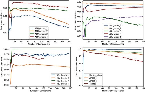
7.4. Factor analysis

Factor Analysis is a linear function transformation dimensionality reduction method and it is based on statistical approaches of PCA (Lavanya and Sanjeevi 2013). This method removes the correlation of original feature concentration through some latent factors that contain a linear combination of original features (Wang and Wang 2015). The contribution of each band is indicated by covariance analysis using this approach. This dimensionality reduction technique observes and interprets the underlying structure of bands through factor scores or components. In our simulations, the number of components of Factor Analysis varies from 2 to 179. Factor Analysis helps improve the AUC of most datasets while using a few components, as indicated by the results for RX detector shown in Figure 20.

Figure 20. AUC evaluation of RX detectors using factor analysis.

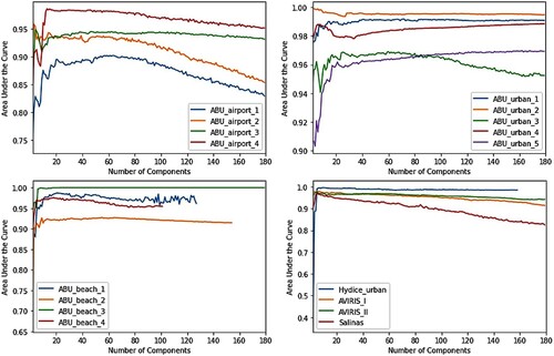
7.5. Isometric mapping

The abovementioned techniques used for dimensionality reduction are linear methods. Several non-linear dimensionality reduction techniques were also presented in the literature such as; Isometric mapping (ISOMAP) (Anowar, Sadaoui, and Selim 2021; Balasubramanian and Schwartz 2002; Tenenbaum, De Silva, and Langford 2000), Kernel PCA (Datta, Ghosh, and Ghosh 2018), t-distributed Stochastic Neighbor Embedding (t-SNE) (Melit Devassy and George 2020), Multidimensional Scaling (MDS) (George and Mallery 2020), Autoencoder (Sakurada and Yairi 2014; Y. Wang, Yao, and Zhao 2016), etc. Therefore, a non-linear ISOMAP technique is also implemented in this study. It converts a higher dimensional space into a lower dimensional space by extracting the intrinsic manifold of hyperspectral data. This technique aims to maintain geodesic distances inside the low dimensional space. By maintaining geodesic proximities that used a non-Euclidean metric, this method retains the nonlinear characteristics of the original data. The geodesic metric precisely estimates the interpoint distances among points on a nonlinear manifold where the data is located (Hannachi and Turner 2013). ISOMAP can learn non-linear embedding which retains the inherent geometry of the data, whereas PCA determines the linear projection which best retains the variance estimated in the input space.

For our simulations, the number of components of ISOMAP is varied from 2 to 70 which is followed by the RX detector. Figure 21 shows the AUC for RX detector w.r.t. number of components.

Figure 21. AUC evaluation of RX detector using ISOMAP.

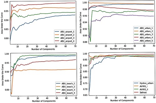
8. Conclusion and future work

In this paper, an extensive review of various anomaly detection techniques is presented. Anomalies are characterized into different types. The existing anomaly detection techniques are categorized into eight types, i.e. Statistics-based, Subspace-based, Kernel-based, Filtering-based, Clustering-based, Low-rank-based, Representation-based and Deep learning-based techniques. Signal models for each of these categories are presented, moreover, a detailed literature review is performed for various anomaly detection techniques. Extensive performance comparison is done using our simulation results while applying the considered anomaly detection techniques to 17 available datasets. The results indicate that the best performance is exhibited by AED, LSAD-CR-IDW, LSUNRSORAD and UNRS as shown by their mean and median AUC values. These conventional approaches aim to increase the detection rate while reducing computation time as well as false alarm rate. The effect of different dimensionality reduction techniques on hyperspectral images is also analyzed in this study. The results of dimensionality reduction techniques, including PCA, ICA, SVD and factor analysis, indicate that 10–30 bands of hyperspectral imagery achieve satisfactory results.

Hyperspectral anomaly detection has attracted a lot of interest in recent years. Despite the advances in anomaly detection algorithms, there are certain limitations, e.g. dataset-specific parameters setting and higher computation time. Parameter setting is one of the crucial steps, and directly influences the detection accuracy of the algorithms. For different types of datasets, a method often has distinct parameter settings for each dataset. Due to this reason, it is necessary to decrease the number of free parameters for future algorithm development to enhance efficiency. Another aspect is the computational cost of algorithms. Approaches such as parallel computation and fast matrix computation may be employed for efficient implementation of these algorithms. In the future, the requirements for hardware implementation may also be considered while designing real-time algorithms.

Acknowledgement

The authors gratefully acknowledge the funding and support received from Pakistan Space and Upper Atmosphere Research Commission.

Disclosure statement

No potential conflict of interest was reported by the author(s).

Data availability statement

All datasets used in this study are publicly available. Links to individual datasets are available at: https://github.com/NomanShahRaza/hyperspectral_anomaly_datasets/.

Additional information

Funding

This work was supported by Pakistan Space and Upper Atmosphere Research Commission [grant number NSP-654-20].

References

- Anowar, F., S. Sadaoui, and B. Selim. 2021. “Conceptual and Empirical Comparison of Dimensionality Reduction Algorithms (PCA, KPCA, LDA, MDS, SVD, LLE, ISOMAP, LE, ICA, t-SNE).” Computer Science Review 40: 100378. doi:10.1016/j.cosrev.2021.100378.
- Arisoy, S., N. M. Nasrabadi, and K. Kayabol. 2021. “GAN-Based Hyperspectral Anomaly Detection.” 2020 28th European Signal Processing Conference (EUSIPCO), 1891–1895.
- Atkinson, P. M., and A. R. L. Tatnall. 1997. “Introduction Neural Networks in Remote Sensing.” International Journal of Remote Sensing 18 (4): 699–709.
- Ayhan, B., M. Dao, C. Kwan, H.-M. Chen, J. F. Bell, and R. Kidd. 2017. “A Novel Utilization of Image Registration Techniques to Process Mastcam Images in Mars Rover with Applications to Image Fusion, Pixel Clustering, and Anomaly Detection.” IEEE Journal of Selected Topics in Applied Earth Observations and Remote Sensing 10 (10): 4553–4564.
- Balasubramanian, M., and E. L. Schwartz. 2002. “The Isomap Algorithm and Topological Stability.” Science 295 (5552): 7. doi:10.1126/science.295.5552.7a.
- Banerjee, A., P. Burlina, and C. Diehl. 2006. “A Support Vector Method for Anomaly Detection in Hyperspectral Imagery.” IEEE Transactions on Geoscience and Remote Sensing 44 (8): 2282–2291.
- Bati, E., A. Çalışkan, A. Koz, and A. A. Alatan. 2015. “Hyperspectral Anomaly Detection Method Based on Auto-Encoder.” Image and Signal Processing for Remote Sensing XXI 9643: 96430N. doi:10.1117/12.2195180.
- Baur, C., B. Wiestler, S. Albarqouni, and N. Navab. 2018. “Deep Autoencoding Models for Unsupervised Anomaly Segmentation in Brain MR Images.” International MICCAI Brainlesion Workshop, 161–169. Part of the Lecture Notes in Computer Science book series (LNIP, volume 11383).
- Bioucas-Dias, J. M., A. Plaza, N. Dobigeon, M. Parente, Q. Du, P. Gader, and J. Chanussot. 2012. “Hyperspectral Unmixing Overview: Geometrical, Statistical, and Sparse Regression-Based Approaches.” IEEE Journal of Selected Topics in Applied Earth Observations and Remote Sensing 5 (2): 354–379.
- Borghys, D., I. Kåsen, V. Achard, and C. Perneel. 2012. “Hyperspectral Anomaly Detection: Comparative Evaluation in Scenes with Diverse Complexity.” Journal of Electrical and Computer Engineering 2012: 1–16.
- Bradley, A. P. 1997. “The Use of the Area under the ROC Curve in the Evaluation of Machine Learning Algorithms.” Pattern Recognition 30 (7): 1145–1159.
- Camps-Valls, G., and L. Bruzzone. 2005. “Kernel-Based Methods for Hyperspectral Image Classification.” IEEE Transactions on Geoscience and Remote Sensing 43 (6): 1351–1362.
- Candès, E. J., X. Li, Y. Ma, and J. Wright. 2011. “Robust Principal Component Analysis?” Journal of the ACM (JACM) 58 (3): 1–37.
- Carlotto, M. J. 2005. “A Cluster-Based Approach for Detecting Man-Made Objects and Changes in Imagery.” IEEE Transactions on Geoscience and Remote Sensing 43 (2): 374–387.
- Chalapathy, R., and S. Chawla. 2019. “Deep Learning for Anomaly Detection: A Survey.” ArXiv Preprint ArXiv:1901.03407.
- Chang, C. I. 2021. “An Effective Evaluation Tool for Hyperspectral Target Detection: 3d Receiver Operating Characteristic Curve Analysis.” IEEE Transactions on Geoscience and Remote Sensing 59 (6): 5131–5153. doi:10.1109/TGRS.2020.3021671.
- Chang, C. I., H. Cao, S. Chen, X. Shang, C. Yu, and M. Song. 2021. “Orthogonal Subspace Projection-Based Go-Decomposition Approach to Finding Low-Rank and Sparsity Matrices for Hyperspectral Anomaly Detection.” IEEE Transactions on Geoscience and Remote Sensing 59 (3): 2403–2429. doi:10.1109/TGRS.2020.3002724.
- Chang, C. I., H. Cao, and M. Song. 2021. “Orthogonal Subspace Projection Target Detector for Hyperspectral Anomaly Detection.” IEEE Journal of Selected Topics in Applied Earth Observations and Remote Sensing 14: 4915–4932. doi:10.1109/JSTARS.2021.3068983.
- Chen, S.-Y., C. Lin, C.-H. Tai, and S.-J. Chuang. 2018. “Adaptive Window-Based Constrained Energy Minimization for Detection of Newly Grown Tree Leaves.” Remote Sensing 10 (1): 96.
- Chen, Y., Z. Lin, X. Zhao, G. Wang, and Y. Gu. 2014. “Deep Learning-Based Classification of Hyperspectral Data.” IEEE Journal of Selected Topics in Applied Earth Observations and Remote Sensing 7 (6): 2094–2107.
- Comon, P. 1994. “Independent Component Analysis, a New Concept?” Signal Processing 36 (3): 287–314.
- Datta, A., S. Ghosh, and A. Ghosh. 2018. “PCA, Kernel PCA and Dimensionality Reduction in Hyperspectral Images.” Advances in Principal Component Analysis: Research and Development, 19–46. doi:10.1007/978-981-10-6704-4_2.
- Du, Q., I. Kopriva, and H. H. Szu. 2006. “Independent-Component Analysis for Hyperspectral Remote Sensing Imagery Classification.” Optical Engineering 45 (1): 017008.
- Du, B., and L. Zhang. 2011. “Random-Selection-Based Anomaly Detector for Hyperspectral Imagery.” IEEE Transactions on Geoscience and Remote Sensing 49 (5): 1578–1589.
- Du, B., R. Zhao, L. Zhang, and L. Zhang. 2016. “A Spectral-Spatial Based Local Summation Anomaly Detection Method for Hyperspectral Images.” Signal Processing 124: 115–131. doi:10.1016/j.sigpro.2015.09.037.
- Faraggi, D., and B. Reiser. 2002. “Estimation of the Area under the ROC Curve.” Statistics in Medicine 21 (20): 3093–3106.
- Fauvel, M., Y. Tarabalka, J. A. Benediktsson, J. Chanussot, and J. C. Tilton. 2013. “Advances in Spectral-Spatial Classification of Hyperspectral Images.” Proceedings of the IEEE 101 (3): 652–675.
- Fawcett, T. 2006. “An Introduction to ROC Analysis.” Pattern Recognition Letters 27 (8): 861–874.
- Feng, S., S. Tang, C. Zhao, and Y. Cui. 2022. “A Hyperspectral Anomaly Detection Method Based on Low-Rank and Sparse Decomposition with Density Peak Guided Collaborative Representation.” IEEE Transactions on Geoscience and Remote Sensing 60: 1–13. doi:10.1109/TGRS.2021.3054736.
- Fu, X., S. Jia, L. Zhuang, M. Xu, J. Zhou, and Q. Li. 2021. “Hyperspectral Anomaly Detection via Deep Plug-and-Play Denoising CNN Regularization.” IEEE Transactions on Geoscience and Remote Sensing 59 (11): 9553–9568. doi:10.1109/TGRS.2021.3049224.
- Gao, C., H. Sun, T. Wang, M. Tang, N. I. Bohnen, M. L. T. M. Müller, T. Herman, et al. 2018. “Model-Based and Model-Free Machine Learning Techniques for Diagnostic Prediction and Classification of Clinical Outcomes in Parkinson’s Disease.” Scientific Reports 8 (1): 1–21.
- George, D., and P. Mallery. 2020. “Multidimensional Scaling.” IBM SPSS Statistics 26 Step by Step, 247–257. doi:10.4324/9780429056765-20.
- Goetz, A. F. H., G. Vane, J. E. Solomon, and B. N. Rock. 1985. “Imaging Spectrometry for Earth Remote Sensing.” Science 228 (4704): 1147–1153.
- Golub, G. H., and C. Reinsch. 1971. “Singular Value Decomposition and Least Squares Solutions.” In Linear Algebra. Handbook for Automatic Computation. Vol. 2, edited by F. L. Bauer, 134–151. Berlin: Springer.
- Guo, Q., B. Zhang, Q. Ran, L. Gao, J. Li, and A. Plaza. 2014. “Weighted-RXD and Linear Filter-Based RXD: Improving Background Statistics Estimation for Anomaly Detection in Hyperspectral Imagery.” IEEE Journal of Selected Topics in Applied Earth Observations and Remote Sensing 7 (6): 2351–2366.
- Hannachi, A., and A. G. Turner. 2013. “Isomap Nonlinear Dimensionality Reduction and Bimodality of Asian Monsoon Convection.” Geophysical Research Letters 40 (8): 1653–1658. doi:10.1002/grl.50351.
- Hansen, P. C. 1990. “Truncated Singular Value Decomposition Solutions to Discrete Ill-Posed Problems with Ill-Determined Numerical Rank.” SIAM Journal on Scientific and Statistical Computing 11 (3): 503–518.
- Harsanyi, J. C., and C.-I. Chang. 1994. “Hyperspectral Image Classification and Dimensionality Reduction: An Orthogonal Subspace Projection Approach.” IEEE Transactions on Geoscience and Remote Sensing 32 (4): 779–785.
- Hoffmann, H. 2007. “Kernel PCA for Novelty Detection.” Pattern Recognition 40 (3): 863–874.
- Huang, Z., L. Fang, and S. Li. 2020. “Subpixel-Pixel-Superpixel Guided Fusion for Hyperspectral Anomaly Detection.” IEEE Transactions on Geoscience and Remote Sensing 58 (9): 5998–6007. doi:10.1109/TGRS.2019.2961703.
- Huang, Q., W. Zhu, Y. Zhao, L. Chen, Y. Wang, T. Yue, and X. Cao. 2018, June. “Multispectral Image Intrinsic Decomposition via Subspace Constraint.” IEEE/CVF Conference on Computer Vision and Pattern Recognition, Salt Lake City, UT, 6430–6439.
- Hussain, M., S. K. Wajid, A. Elzaart, and M. Berbar. 2011. “A Comparison of SVM Kernel Functions for Breast Cancer Detection.” 2011 Eighth International Conference Computer Graphics, Imaging and Visualization, 145–150.
- Huyan, N., X. Zhang, H. Zhou, and L. Jiao. 2019. “Hyperspectral Anomaly Detection via Background and Potential Anomaly Dictionaries Construction.” IEEE Transactions on Geoscience and Remote Sensing 57 (4): 2263–2276. doi:10.1109/TGRS.2018.2872590.
- Hytla, P. C., R. C. Hardie, M. T. Eismann, and J. Meola. 2009. “Anomaly Detection in Hyperspectral Imagery: Comparison of Methods Using Diurnal and Seasonal Data.” Journal of Applied Remote Sensing 3 (1): 033546.
- Hyvarinen, A. 1999. “Fast and Robust Fixed-Point Algorithms for Independent Component Analysis.” IEEE Transactions on Neural Networks 10 (3): 626–634.
- Hyvärinen, A., and E. Oja. 2000. “Independent Component Analysis: Algorithms and Applications.” Neural Networks 13 (4–5): 411–430.
- Kang, X., X. Zhang, S. Li, K. Li, J. Li, and J. A. Benediktsson. 2017. “Hyperspectral Anomaly Detection with Attribute and Edge-Preserving Filters.” IEEE Transactions on Geoscience and Remote Sensing 55 (10): 5600–5611.
- Kåsen, I., A. Rødningsby, T. V. Haavardsholm, and T. Skauli. 2008. “Band Selection for Hyperspectral Target Detection Based on a Multinormal Mixture Anomaly Detection Algorithm.” Algorithms and Technologies for Multispectral, Hyperspectral, and Ultraspectral Imagery XIV, 6966, 696606.
- Keerthi, S. S., and C.-J. Lin. 2003. “Asymptotic Behaviors of Support Vector Machines with Gaussian Kernel.” Neural Computation 15 (7): 1667–1689.
- Khan, M. J., H. S. Khan, A. Yousaf, K. Khurshid, and A. Abbas. 2018. “Modern Trends in Hyperspectral Image Analysis: A Review.” IEEE Access 6: 14118–14129.
- Khazai, S., A. Safari, B. Mojaradi, and S. Homayouni. 2013. “An Approach for Subpixel Anomaly Detection in Hyperspectral Images.” IEEE Journal of Selected Topics in Applied Earth Observations and Remote Sensing 6 (2): 769–778. doi:10.1109/JSTARS.2012.2210277.
- Kiran, B. R., D. M. Thomas, and R. Parakkal. 2018. “An Overview of Deep Learning Based Methods for Unsupervised and Semi-Supervised Anomaly Detection in Videos.” Journal of Imaging 4 (2): 36.
- Klema, V., and A. Laub. 1980. “The Singular Value Decomposition: Its Computation and Some Applications.” IEEE Transactions on Automatic Control 25 (2): 164–176.
- Kolda, T. G., and B. W. Bader. 2009. “Tensor Decompositions and Applications.” SIAM Review 51 (3): 455–500.
- Küçük, S., and S. E. Yüksel. 2015. “Comparison of RX-Based Anomaly Detectors on Synthetic and Real Hyperspectral Data.” 2015 7th Workshop on Hyperspectral Image and Signal Processing: Evolution in Remote Sensing (WHISPERS), 1–4.
- Kwon, H., and N. M. Nasrabadi. 2005. “Kernel RX-Algorithm: A Nonlinear Anomaly Detector for Hyperspectral Imagery.” IEEE Transactions on Geoscience and Remote Sensing 43 (2): 388–397.
- Lavanya, A., and S. Sanjeevi. 2013. “An Improved Band Selection Technique for Hyperspectral Data Using Factor Analysis.” Journal of the Indian Society of Remote Sensing 41 (2): 199–211.
- Li, W., and Q. Du. 2013. “Unsupervised Nearest Regularized Subspace for Anomaly Detection in Hyperspectral Imagery.” 2013 IEEE International Geoscience and Remote Sensing Symposium-IGARSS, 1055–1058.
- Li, W., and Q. Du. 2015. “Collaborative Representation for Hyperspectral Anomaly Detection.” IEEE Transactions on Geoscience and Remote Sensing 53 (3): 1463–1474.
- Li, Shuangjiang, W. Wang, H. Qi, B. Ayhan, C. Kwan, and S. Vance. 2015. “Low-Rank Tensor Decomposition Based Anomaly Detection for Hyperspectral Imagery.” Proceedings – International Conference on Image Processing, ICIP, 2015-December, 4525–4529. doi:10.1109/ICIP.2015.7351663.
- Li, W., G. Wu, and Q. Du. 2017. “Transferred Deep Learning for Anomaly Detection in Hyperspectral Imagery.” IEEE Geoscience and Remote Sensing Letters 14 (5): 597–601.
- Li, Shutao, K. Zhang, P. Duan, and X. Kang. 2019. “Hyperspectral Anomaly Detection with Kernel Isolation Forest.” IEEE Transactions on Geoscience and Remote Sensing 58 (1): 319–329.
- Li, Shutao, K. Zhang, Q. Hao, P. Duan, and X. Kang. 2018. “Hyperspectral Anomaly Detection with Multiscale Attribute and Edge-Preserving Filters.” IEEE Geoscience and Remote Sensing Letters 15 (10): 1605–1609.
- Li, J., H. Zhang, L. Zhang, and L. Ma. 2015. “Hyperspectral Anomaly Detection by the Use of Background Joint Sparse Representation.” IEEE Journal of Selected Topics in Applied Earth Observations and Remote Sensing 8 (6): 2523–2533. doi:10.1109/JSTARS.2015.2437073.
- Lin, H.-T., and C.-J. Lin. 2003. “A Study on Sigmoid Kernels for SVM and the Training of non-PSD Kernels by SMO-Type Methods.” Neural Computation 3 (1–32): 16.
- Liu, W., and C.-I. Chang. 2004. “A Nested Spatial Window-Based Approach to Target Detection for Hyperspectral Imagery.” IGARSS 2004. 2004 IEEE International Geoscience and Remote Sensing Symposium, 1.
- Liu, W.-M., and C.-I. Chang. 2013. “Multiple-Window Anomaly Detection for Hyperspectral Imagery.” IEEE Journal of Selected Topics in Applied Earth Observations and Remote Sensing 6 (2): 644–658.
- Liu, D., and L. Han. 2017. “Spectral Curve Shape Matching Using Derivatives in Hyperspectral Images.” IEEE Geoscience and Remote Sensing Letters 14 (4): 504–508.
- Liu, J., Z. Hou, W. Li, R. Tao, D. Orlando, and H. Li. 2022. “Multipixel Anomaly Detection with Unknown Patterns for Hyperspectral Imagery.” IEEE Transactions on Neural Networks and Learning Systems 33: 5557–5567. doi:10.1109/TNNLS.2021.3071026.
- Ma, N., Y. Peng, S. Wang, and P. H. W. Leong. 2018. “An Unsupervised Deep Hyperspectral Anomaly Detector.” Sensors 18 (3): 693.
- Maji, S., A. C. Berg, and J. Malik. 2008. “Classification Using Intersection Kernel Support Vector Machines Is Efficient.” 2008 IEEE Conference on Computer Vision and Pattern Recognition, 1–8.
- Makki, I., R. Younes, C. Francis, T. Bianchi, and M. Zucchetti. 2017. “A Survey of Landmine Detection Using Hyperspectral Imaging.” ISPRS Journal of Photogrammetry and Remote Sensing 124: 40–53.
- Manolakis, D. 2005. “Taxonomy of Detection Algorithms for Hyperspectral Imaging Applications.” Optical Engineering 44 (6): 066403. doi:10.1117/1.1930927.
- Matteoli, S., M. Diani, and G. Corsini. 2010. “A Tutorial Overview of Anomaly Detection in Hyperspectral Images.” IEEE Aerospace and Electronic Systems Magazine 25 (7 PART 2): 5–28. doi:10.1109/MAES.2010.5546306.
- Melit Devassy, B., and S. George. 2020. “Dimensionality Reduction and Visualisation of Hyperspectral Ink Data Using t-SNE.” Forensic Science International 311: 110194. doi:10.1016/j.forsciint.2020.110194.
- Molero, J. M., E. M. Garzón, I. Garcia, and A. J. Plaza. 2012. “Anomaly Detection Based on a Parallel Kernel RX Algorithm for Multicore Platforms.” Journal of Applied Remote Sensing 6 (1): 061503.
- Nasrabadi, N. M. 2014. “Hyperspectral Target Detection: An Overview of Current and Future Challenges.” IEEE Signal Processing Magazine 31 (1): 34–44. doi:10.1109/MSP.2013.2278992.
- Ng, A. 2011. “Sparse Autoencoder.” CS294A Lecture Notes 72: 1–19.
- Noble, W. S. 2006. “What Is a Support Vector Machine?” Nature Biotechnology 24 (12): 1565–1567.
- Pal, M. 2005. “Random Forest Classifier for Remote Sensing Classification.” International Journal of Remote Sensing 26 (1): 217–222.
- Pearson, K. 1901. “LIII. On Lines and Planes of Closest fit to Systems of Points in Space.” The London, Edinburgh, and Dublin Philosophical Magazine and Journal of Science 2 (11): 559–572.
- Qu, Y., W. Wang, R. Guo, B. Ayhan, C. Kwan, S. Vance, and H. Qi. 2018. “Hyperspectral Anomaly Detection through Spectral Unmixing and Dictionary-Based Low-Rank Decomposition.” IEEE Transactions on Geoscience and Remote Sensing 56 (8): 4391–4405.
- Racetin, I., and A. Krtalić. 2021. “Systematic Review of Anomaly Detection in Hyperspectral Remote Sensing Applications.” Applied Sciences 11 (11), doi:10.3390/app11114878.
- Rao, W., L. Gao, Y. Qu, X. Sun, B. Zhang, and J. Chanussot. 2022a. “Siamese Transformer Network for Hyperspectral Image Target Detection.” IEEE Transactions on Geoscience and Remote Sensing 60: 1–19. doi:10.1109/TGRS.2022.3163173.
- Rao, W., Y. Qu, L. Gao, X. Sun, Y. Wu, and B. Zhang. 2022b. “Transferable Network with Siamese Architecture for Anomaly Detection in Hyperspectral Images.” International Journal of Applied Earth Observation and Geoinformation 106: 102669. doi:10.1016/j.jag.2021.102669.
- Reed, I. S., and X. Yu. 1990. “Adaptive Multiple-Band CFAR Detection of an Optical Pattern with Unknown Spectral Distribution.” IEEE Transactions on Acoustics, Speech, and Signal Processing 38 (10): 1760–1770.
- Reynolds, D. A. 2009. “Gaussian Mixture Models.” Encyclopedia of Biometrics 741: 659–663.
- Rodarmel, C., and J. Shan. 2002. “Principal Component Analysis for Hyperspectral Image Classification.” Surveying and Land Information Science 62 (2): 115–122.
- Sakurada, M., and T. Yairi. 2014. “Anomaly Detection Using Autoencoders with Nonlinear Dimensionality Reduction.” ACM International Conference Proceeding Series, 02-December-2014, 4–11. doi:10.1145/2689746.2689747.
- Salem, M. Ben, K. S. Ettabaa, and M. A. Hamdi. 2014, November 5–7. “Anomaly Detection in Hyperspectral Imagery: An Overview.” IEEE 2014 First International Image Processing, Applications and Systems Conference (IPAS), Sfax, Tunisia, 1–6. doi:10.1109/ipas.2014.7043320
- Schaum, A. 2004. “Joint Subspace Detection of Hyperspectral Targets.” 2004 IEEE Aerospace Conference Proceedings (IEEE Cat. No. 04TH8720), 3.
- Schaum, A. P. 2007. “Hyperspectral Anomaly Detection Beyond RX.” Algorithms and Technologies for Multispectral, Hyperspectral, and Ultraspectral Imagery XIII 6565: 656502.
- Scholkopf, B., K.-K. Sung, C. J. C. Burges, F. Girosi, P. Niyogi, T. Poggio, and V. Vapnik. 1997. “Comparing Support Vector Machines with Gaussian Kernels to Radial Basis Function Classifiers.” IEEE Transactions on Signal Processing 45 (11): 2758–2765.
- Schölkopf, B., R. C. Williamson, A. J. Smola, J. Shawe-Taylor, and J. C. Platt. 1999. “Support Vector Method for Novelty Detection.” NIPS 12: 582–588.
- Seeböck, P., S. Waldstein, S. Klimscha, B. S. Gerendas, R. Donner, T. Schlegl, U. Schmidt-Erfurth, and G. Langs. 2016. “Identifying and Categorizing Anomalies in Retinal Imaging Data.” ArXiv Preprint ArXiv:1612.00686.
- Shen, S. S., and E. M. Bassett III. 2002. “Information-Theory-Based Band Selection and Utility Evaluation for Reflective Spectral Systems.” Algorithms and Technologies for Multispectral, Hyperspectral, and Ultraspectral Imagery VIII 4725: 18–29.
- Smits, G. F., and E. M. Jordaan. 2002. “Improved SVM Regression Using Mixtures of Kernels.” Proceedings of the 2002 International Joint Conference on Neural Networks. IJCNN’02 (Cat. No. 02CH37290), 3, 2785–2790.
- Souza, C. R. 2010. “Kernel Functions for Machine Learning Applications.” Creative Commons Attribution-Noncommercial-Share Alike, 3, 29.
- Spearman, C. 1961. ““General Intelligence” Objectively Determined and Measured.” The American Journal of Psychology 15 (2): 201–293.
- Stein, D. W. J., S. G. Beaven, L. E. Hoff, E. M. Winter, A. P. Schaum, and A. D. Stocker. 2002. “Anomaly Detection from Hyperspectral Imagery.” IEEE Signal Processing Magazine 19 (1): 58–69.
- Su, H., Z. Wu, H. Zhang, and Q. Du. 2022. “Hyperspectral Anomaly Detection: A Survey.” IEEE Geoscience and Remote Sensing Magazine 10: 64–90. doi:10.1109/MGRS.2021.3105440.
- Sun, W., C. Liu, J. Li, Y. M. Lai, and W. Li. 2014. “Low-Rank and Sparse Matrix Decomposition-Based Anomaly Detection for Hyperspectral Imagery.” Journal of Applied Remote Sensing 8 (1): 083641.
- Sun, X., Y. Qu, L. Gao, X. Sun, H. Qi, B. Zhang, and T. Shen. 2021. “Target Detection through Tree-Structured Encoding for Hyperspectral Images.” IEEE Transactions on Geoscience and Remote Sensing 59 (5): 4233–4249. doi:10.1109/TGRS.2020.3024852.
- Sun, X., Y. Qu, L. Gao, X. Sun, H. Qi, B. Zhang, and T. Shen. 2022. “Ensemble-Based Information Retrieval with Mass Estimation for Hyperspectral Target Detection.” IEEE Transactions on Geoscience and Remote Sensing 60: 1–23. doi:10.1109/TGRS.2021.3075583.
- Taghipour, A., and H. Ghassemian. 2019. “Unsupervised Hyperspectral Target Detection Using Spectral Residual of Deep Autoencoder Networks.” 2019 4th International Conference on Pattern Recognition and Image Analysis (IPRIA), 52–57.
- Tan, K., Z. Hou, F. Wu, Q. Du, and Y. Chen. 2019. “Anomaly Detection for Hyperspectral Imagery Based on the Regularized Subspace Method and Collaborative Representation.” Remote Sensing 11 (11): 1318.
- Tang, Y. Y., Y. Lu, and H. Yuan. 2015. “Hyperspectral Image Classification Based on Three-Dimensional Scattering Wavelet Transform.” IEEE Transactions on Geoscience and Remote Sensing 53 (5): 2467–2480.
- Tao, R., X. Zhao, W. Li, H.-C. Li, and Q. Du. 2019. “Hyperspectral Anomaly Detection by Fractional Fourier Entropy.” IEEE Journal of Selected Topics in Applied Earth Observations and Remote Sensing 12 (12): 4920–4929.
- Tenenbaum, J. B., V. De Silva, and J. C. Langford. 2000. “A Global Geometric Framework for Nonlinear Dimensionality Reduction.” Science 290 (5500): 2319–2323. doi:10.1126/science.290.5500.2319.
- Theiler, J., and B. Wohlberg. 2012. “Local Coregistration Adjustment for Anomalous Change Detection.” IEEE Transactions on Geoscience and Remote Sensing 50 (8): 3107–3116.
- Thurstone, L. L. 1947, December 4. Multiple-Factor Analysis; A Development and Expansion of the Vectors of Mind. The Quarterly Review of Biology. Chicago: The University of Chicago Press.
- Tu, B., N. Li, Z. Liao, X. Ou, and G. Zhang. 2019. “Hyperspectral Anomaly Detection via Spatial Density Background Purification.” Remote Sensing 11(12): 2618. doi:10.3390/rs11222618.
- Tu, B., X. Yang, N. Li, C. Zhou, and D. He. 2020a. “Hyperspectral Anomaly Detection via Density Peak Clustering.” Pattern Recognition Letters 129: 144–149.
- Tu, B., X. Yang, C. Zhou, D. He, and A. Plaza. 2020b. “Hyperspectral Anomaly Detection Using Dual Window Density.” IEEE Transactions on Geoscience and Remote Sensing 58 (12): 8503–8517.
- Van Der Maaten, L., E. Postma, and J. den Herik. 2009. “Dimensionality Reduction: A Comparative.” Journal of Machine Learning Research 10 (66–71): 13.
- Verdoja, F., and M. Grangetto. 2020. “Graph Laplacian for Image Anomaly Detection.” Machine Vision and Applications 31 (1): 1–16.
- Waheed, T., R. B. Bonnell, S. O. Prasher, and E. Paulet. 2006. “Measuring Performance in Precision Agriculture: CART—A Decision Tree Approach.” Agricultural Water Management 84 (1–2): 173–185.
- Wall, M. E., A. Rechtsteiner, and L. M. Rocha. 2003. “Singular Value Decomposition and Principal Component Analysis.” In A Practical Approach to Microarray Data Analysis, edited by D. P. Berrar, W. Dubitzky, and M. Granzow, 91–109. Boston, MA: Springer.
- Wang, R., H. Hu, F. He, F. Nie, S. Cai, and Z. Ming. 2020. “Self-Weighted Collaborative Representation for Hyperspectral Anomaly Detection.” Signal Processing 177: 107718. doi:10.1016/j.sigpro.2020.107718.
- Wang, Y.-X., J.-X. Liu, Y.-L. Gao, C.-H. Zheng, and J.-L. Shang. 2016. “Differentially Expressed Genes Selection via Laplacian Regularized Low-Rank Representation Method.” Computational Biology and Chemistry 65: 185–192.
- Wang, Shuangting, and C. Wang. 2015. “Research on Dimension Reduction Method for Hyperspectral Remote Sensing Image Based on Global Mixture Coordination Factor Analysis.” International Archives of the Photogrammetry, Remote Sensing & Spatial Information Sciences 40: 159–167.
- Wang, Shaoyu, X. Wang, L. Zhang, and Y. Zhong. 2022a. “Auto-AD: Autonomous Hyperspectral Anomaly Detection Network Based on Fully Convolutional Autoencoder.” IEEE Transactions on Geoscience and Remote Sensing 60: 1–14. doi:10.1109/TGRS.2021.3057721.
- Wang, Shaoyu, X. Wang, L. Zhang, and Y. Zhong. 2022b. “Deep Low-Rank Prior for Hyperspectral Anomaly Detection.” IEEE Transactions on Geoscience and Remote Sensing 60: 1–17. doi:10.1109/TGRS.2022.3165833.
- Wang, Y., H. Yao, and S. Zhao. 2016. “Auto-Encoder Based Dimensionality Reduction.” Neurocomputing 184: 232–242. doi:10.1016/j.neucom.2015.08.104.
- Wold, S., K. Esbensen, and P. Geladi. 1987. “Principal Component Analysis.” Chemometrics and Intelligent Laboratory Systems 2 (1–3): 37–52.
- Xie, W., T. Jiang, Y. Li, X. Jia, and J. Lei. 2019a. “Structure Tensor and Guided Filtering-Based Algorithm for Hyperspectral Anomaly Detection.” IEEE Transactions on Geoscience and Remote Sensing 57 (7): 4218–4230.
- Xie, W., J. Lei, B. Liu, Y. Li, and X. Jia. 2019b. “Spectral Constraint Adversarial Autoencoders Approach to Feature Representation in Hyperspectral Anomaly Detection.” Neural Networks 119: 222–234. doi:10.1016/j.neunet.2019.08.012.
- Xie, W., B. Liu, Y. Li, J. Lei, C.-I. Chang, and G. He. 2020a. “Spectral Adversarial Feature Learning for Anomaly Detection in Hyperspectral Imagery.” IEEE Transactions on Geoscience and Remote Sensing 58 (4): 2352–2365.
- Xie, W., B. Liu, Y. Li, J. Lei, and Q. Du. 2020b. “Autoencoder and Adversarial-Learning-Based Semisupervised Background Estimation for Hyperspectral Anomaly Detection.” IEEE Transactions on Geoscience and Remote Sensing 58 (8): 5416–5427.
- Xie, W., X. Zhang, Y. Li, J. Lei, J. Li, and Q. Du. 2021. “Weakly Supervised Low-Rank Representation for Hyperspectral Anomaly Detection.” IEEE Transactions on Cybernetics 51 (8): 3889–3900. doi:10.1109/TCYB.2021.3065070.
- Xu, Y., Z. Wu, J. Li, A. Plaza, and Z. Wei. 2016. “Anomaly Detection in Hyperspectral Images Based on Low-Rank and Sparse Representation.” IEEE Transactions on Geoscience and Remote Sensing 54 (4): 1990–2000.
- Yang, C., J. K. Westbrook, C. P.-C. Suh, D. E. Martin, W. C. Hoffmann, Y. Lan, B. K. Fritz, and J. A. Goolsby. 2014. “An Airborne Multispectral Imaging System Based on Two Consumer-Grade Cameras for Agricultural Remote Sensing.” Remote Sensing 6 (6): 5257–5278.
- Yousefan, M., H. E. Najafabadi, H. Amirkhani, H. Leung, and V. Hajihashemi. 2022. “Deep Anomaly Detection in Hyperspectral Images Based on Membership Maps and Object Area Filtering.” Expert Systems with Applications 191: 116200.
- Yuan, Y., Q. Wang, and G. Zhu. 2015. “Fast Hyperspectral Anomaly Detection via High-Order 2-D Crossing Filter.” IEEE Transactions on Geoscience and Remote Sensing 53 (2): 620–630.
- Zhang, L., and B. Cheng. 2019. “A Stacked Autoencoders-Based Adaptive Subspace Model for Hyperspectral Anomaly Detection.” Infrared Physics & Technology 96: 52–60.
- Zhang, W., X. Lu, and X. Li. 2019. “Similarity Constrained Convex Nonnegative Matrix Factorization for Hyperspectral Anomaly Detection.” IEEE Transactions on Geoscience and Remote Sensing 57 (7): 4810–4822.
- Zhao, R., B. Du, and L. Zhang. 2014. “A Robust Nonlinear Hyperspectral Anomaly Detection Approach.” IEEE Journal of Selected Topics in Applied Earth Observations and Remote Sensing 7 (4): 1227–1234.
- Zhao, C., C. Li, S. Feng, N. Su, and W. Li. 2020. “A Spectral-Spatial Anomaly Target Detection Method Based on Fractional Fourier Transform and Saliency Weighted Collaborative Representation for Hyperspectral Images.” IEEE Journal of Selected Topics in Applied Earth Observations and Remote Sensing 13: 5982–5997. doi:10.1109/JSTARS.2020.3028372.
- Zhao, C., Y. Wang, B. Qi, and J. Wang. 2015. “Global and Local Real-Time Anomaly Detectors for Hyperspectral Remote Sensing Imagery.” Remote Sensing 7 (4): 3966–3985.
- Zhao, C., and L. Zhang. 2018. “Spectral-Spatial Stacked Autoencoders Based on Low-Rank and Sparse Matrix Decomposition for Hyperspectral Anomaly Detection.” Infrared Physics & Technology 92: 166–176. doi:10.1016/j.infrared.2018.06.001.
- Zhou, J., C. Kwan, B. Ayhan, and M. T. Eismann. 2016. “A Novel Cluster Kernel RX Algorithm for Anomaly and Change Detection Using Hyperspectral Images.” IEEE Transactions on Geoscience and Remote Sensing 54 (11): 6497–6504. doi:10.1109/TGRS.2016.2585495.
- Zhou, T., and D. Tao. 2011. “Godec: Randomized Low-Rank & Sparse Matrix Decomposition in Noisy Case.” Proceedings of the 28th International Conference on Machine Learning, ICML 2011.
- Zhuang, L., L. Gao, B. Zhang, X. Fu, and J. M. Bioucas-Dias. 2021. “Hyperspectral Image Denoising and Anomaly Detection Based on Low-Rank and Sparse Representations.” IEEE Transactions on Geoscience and Remote Sensing 60: 1–17. doi:10.1109/TGRS.2020.3040221.
- Zou, K. H., S. K. Warfield, A. Bharatha, C. M. C. Tempany, M. R. Kaus, S. J. Haker, W. M. Wells III, F. A. Jolesz, and R. Kikinis. 2004. “Statistical Validation of Image Segmentation Quality Based on a Spatial Overlap Index1: Scientific Reports.” Academic Radiology 11 (2): 178–189.