Mapping the spatial and temporal patterns of fallow land in mountainous regions of China

ABSTRACT

The rapid growth of the global population has resulted in a continuous increase in cropland intensity and a shortening of the fallow period as part of the cropland rotation cycle. Yet, there is a lack of systematic knowledge on the extent of fallow lands, particularly in complex landscapes, such as the mountainous regions of China. To fill this knowledge gap, taking Yuanyang County (YYC), Yunnan Province, China, as a case study, we tested a method to identify the spatial-temporal distribution of fallow land by mapping cropland with Landsat data. The overall accuracy of land cover classification, including cropland, ranged between 90.1% and 95.8% from 1998 to 2019. The average accuracy of fallow plots was 75.7% from 2001 to 2019. The annual fallow rate varied between 8.3% and 54.3%, with an average of 20.7%. Kernel density estimated with the probability density function showed that fallow varied between 5 and 13 blocks per km², gradually decreasing from the central area to the periphery. Increasing elevation, the low value of regional domestic products, and the increased distance to rural settlements were closely related to the higher proportions of fallow land. The approach presented here can be applied to map fallow land in other regions.

KEYWORDS:

• Remote sensing
• fallow land
• kernel density
• time series
• China

1. Introduction

With an increasing global population, food security has become a hot topic (Prosekov and Ivanova 2018). One of the solutions to meet the growing demand for agricultural commodities is to intensify agricultural production, for example, by reducing crop rotation with clean and green fallowing (Wang et al. 2020). However, an increase in cropping intensity may lead to addition problems, such as declined soil quality, soil compaction and erosion, and pollution through the excessive use of fertilizers and herbicides (Song and Pijanowski 2014; Song and Deng 2017). To maintain the productive capacity and ecological quality of cropland, several countries have developed clean and green fallow policies, such as the America Conservation Reserve Program (Sullivan et al. 2004), the Japan Rice Paddy Set-aside Program (Sato 2001), and the EU McSharry Reforms (Groier 2000). Such an approach can improve cropland quality, thereby increasing the agricultural production potential (Brinson and Eckles 2011). In addition, fallow can also produce various ecological and environmental benefits and improve the quality of water resources and air (van Vliet et al. 2012), which is particularly important in some areas of China with a high cropping intensity (Wu and Xie 2017).

Fallow areas are generally fields that remain idle for a certain period (Girard et al. 1994; Styger et al. 2007; Babu et al. 2020); they can be classified based on idle time (duration) and idle nature (land cover). The fallow period, as a part of crop rotation, is often short and depends on the agricultural system (Styger et al. 2007; Babu et al. 2020). During the fallow period, which can be a part of crop rotation and replenishment, green manure crops are generally planted; however, crop fields can be transformed into grassland, shrubbery, or even bare lands (Nguyen et al. 2021). In such cases, fallow land can be confused with other land types, e.g. grassland and bare land (Rasul et al. 2018). However, abandoned croplands, in contrast to fallow lands, are generally abandoned for a considerably longer period and characterized by the voluntary or involuntary cessation of farming with the spontaneous recovery of pioneer vegetation, such as grasses, shrubs, and young trees, particularly in the mountainous areas of Southern China (Han and Song 2019). The abandoned plot is considered to have remained without any signs of cultivation for at least several years after cultivation.

To document fallow lands, two methods are commonly used (Ram and Kolarkar 1993; Gumma et al. 2018; Zambon et al. 2018): statistical surveys and satellite remote sensing monitoring. Among the statistical surveying options are household surveys, which can be obtained rapidly via fallow land sampling data (e.g. area and time). However, point-based location data are discrete and lack a relevant spatial context (Shi et al. 2019). In this regard, satellite remote sensing is a valuable technology to identify fallow lands, for instance, by benefiting from texture, reflectance, and spatial associations of picture elements (pixels) (Conrad et al. 2014; Siachalou, Mallinis, and Tsakiri-Strati 2017). Using Landsat imagery, satellite remote sensing allows the retrospective reconstruction of fallow dynamics dating back to as early as the 1980s (Song 2019).

The durations of the cropping and fallow periods are central to identifying fallow fields (Rahman and Saha 2009; Manzungu and Mtali 2012). Using remote sensing technology, different stages of cropland development can be identified alongside the cessation of farming activities which lead to rotational fallow and land abandonment. For example, Rahman and Saha (2009) used Landsat TM and IRS P6 LISS III satellite data to map land cover types in Bangladesh for the identification and analysis of the distribution of fallow fields over a period of 16 years from 1988/89 to 2004/05. Remote sensing technology has also been used to map land cover patterns and identify fallow lands over several periods in Zimbabwe (Manzungu and Mtali 2012). In India, Landsat 8 OLI and Sentinel-1 data have been used to extract actively cropland and fallow rice fields in Odisha (Chandna and Mondal 2020). Although there has been some progress in using remote sensing data to identify fallow lands in China, relevant studies are scarce (Zhang, Li, and Song 2014; Han and Song 2019). In particular, there are no studies that obtained long-term fallow land data and determined the distribution status of fallow lands, particularly in mountainous areas.

Despite the progress in the application of satellite remote sensing in mapping fallow fields, the developed approaches are difficult to implement in mountainous areas. More specifically, in China, mountainous regions are generally characterized by small-scale farming and different degrees of land-use intensity. These areas can be prone to agricultural land abandonment (complete cessation of farming followed by natural recovery), which requires additional efforts in the accurate separation of abandoned fields from temporally fallow fields as a part of crop rotation.

For this study, we selected Yuanyang County (YYC), Honghe Prefecture, Yunnan Province, China, to investigate the spatial and temporal distribution of fallow land. The research objectives are as follows: (1) to develop a remote sensing approach to map the timing of following and the extent of fallow lands, (2) using kernel density analysis to reveal the temporal–spatial characteristics of fallowing, and (3) present the spatial distribution of fallow lands in the context of biophysical factors (topography) and economic aspects (contrasting with regional domestic product – RDP) and distance to settlements (a proxy for travel costs).

2. Materials and methods

2.1. Study area

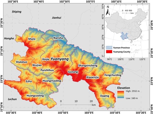
Yuanyang County is located at 102°27′E-103°13′E and 22°49′N-23°19′N, covering a total area of 2,189.88 km². It is the core area of the Red River Hani Terrace (Figure 1), with 3 towns and 11 townships under its jurisdiction. The county is mountainous with undulating terrain, ranging from 160 to 2,932 m above sea level, with an average of 1,304 m. Clouds are common all year round; the average annual temperature is 24°C, with an average annual precipitation of 899 mm. Two or three crops can be harvested annually (Liu et al. 2013).

Figure 1. Geographical location of Yuanyang County.

From 1978 to 2018, the economy and population of YYC have steadily increased (Yuanyang County People’s Government Office 2020). From 1984 to 2018, the population of YYC has increased by 47.9%. In addition, in 2018, the county-level RDP in YYC, converted to the 1978 constant price, had increased 39 times compared to the 1978 level. Especially after 2005, the economy of YYC has been growing rapidly. The structural changes in the economy from 1978 to 2018 have mainly manifested in the rapid decline in the proportion of primary industries (e.g. agriculture), whereas the proportion of secondary and tertiary industries (e.g. service sector) gradually increased. As a consequence, the proportion of agriculture in the RDP in YYC decreased from 1978 to 2018. In 2021, YYC has still largely maintained its terraced agricultural landscapes.

2.2. Data sets

We used nine remotely sensed data sets and products (Table 1): (1) the Landsat series (Masek et al. 2006; Vermote et al. 2016) and their derivatives for land cover classification; (2) very-high resolution (VHR) images, available from Google Earth mapping service, for training and validation data collection; (3) the digital elevation model (DEM), obtained from Google Earth elevation data, for spatial analyses; (4) China land use/cover change (CNLUCC) (Xu et al. 2018) from the Resource and Environmental Science Data Registration and Publishing System, based on Landsat images with overall accuracy (OA) of more than 94%; (5) the 30-meter resolution global land cover data product (GlobeLand30) (Chen et al. 2015) with OAs of 83.50% in 2010 and 85.72% in 2020, classified based on Landsat, HJ-1, and GF-1; (6) global food security-support analysis data (GFSAD) (Zhong et al. 2017), the 2015 global cropland data identified by using multiple remote sensing data and vegetation characteristics, with an OA of 93%; (7) the global forest cover map (GFCM) (Zhang et al. 2019) from the Google Earth Engine platform with an OA above 85%; (8) ten-meter finer resolution observation and monitoring-global land cover (FROM-GLC10) (Gong et al. 2019), produced by classifying ESA Copernicus Sentinel-2 satellite images with an OA of 72.43%. Five different types of land-use/cover change data sets ((4)–(8)) were used combined with VHR satellite imagery from Google Earth mapping service for generation and assignment of thematic classes training and validation data; (9) the spatial distribution of the regional domestic product (RDP) (Xu 2017), part of the China GDP spatial distribution kilometer grid dataset, was weighted by county-level land use data, nighttime light remote sensing data (e.g. DMSP/OLS and NPP/VIIRS), and settlement density data.

Table 1. Remotely sensed datasets used in this study.

Product	Publisher/Data Source	Time coverage	Resolution (m)
Landsat	U.S. Geological Survey https://www.usa.gov/	1998–2019	30
VHR Images*	Google Earth	2009–2019	2.3
DEM*	Google Earth	–	7.5
CNLUCC	Chinese Academy of Sciences http://www.resdc.cn/	2000; 2005; 2010; 2015	30
GlobeLand30	National Geomatics Center of China http://www.globeland30.com/	2010	30
GFSAD	National Aeronautics and Space Administration https://www.croplands.org/	2015	30
GFCM	National Remote Sensing Centre of China http://www.chinageoss.cn/	2018	30
FROM-GLC10	Tsinghua University http://data.ess.tsinghua.edu.cn/	2017	10
RDP	Chinese Academy of Sciences http://www.resdc.cn/	2000; 2005; 2010; 2015	1000

Notes: All datasets in the table are in raster format; VHR: Very-high-resolution data; CNLUCC: China land use/cover change; GlobeLand30: 30-meter resolution global land cover data product; GFSAD: Global Food Security-Support Analysis Data; GFCM: Global Forest Cover Map; FROM-GLC10: Finer Resolution Observation and Monitoring-Global Land Cover; RDP: Regional domestic products. * Google provided raw data for the VHR images and DEM, and the 91wemap software (https://www.91wemap.com) was used to download data. The VHR images represented mosaics of QuickBird, GeoEye-1, and WorldView.

3. Methods

3.1. Mapping fallow lands framework

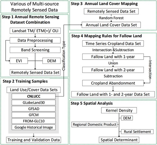
The fallow period in YYC might vary from one to two years. We applied the land cover transfer matrix to calculate the fallow range, using the following steps to identify fallow lands (Figure 2): (1) Pre-processing of the Landsat data to generate the enhanced vegetation index (EVI), combined with multi-band and DEM data to improve the accuracy of classification into actively cultivated and fallowed fields; (2) training and validation data were obtained from all types of remotely sensed products and VHR images; (3) the annual land cover from 1998 to 2019 was interpreted and validated; (4) for the period from 2001 to 2019, the fallow land was mapped by the extent of cropland and the fallow duration; (5) the key spatial features were used to analyze the spatial determinants of fallow lands.

Figure 2. Flowchart showing the classification of fallow land.

3.2. Data set construction and land cover interpretation

Landsat series and first-level data were obtained from the U.S. Geological Survey and pre-processed using the ENVI 5.3 software, including radiometric correction and fast line-of-sight atmospheric analysis of spectral hypercubes (Felde et al. 2003), image co-registration, and subsetting the images to the boundaries of YYC from 1998 to 2019. Because of the presence of clouds, clouds were removed with Fmask algorithm (Zhu, Wang, and Woodcock 2015) and cloud-free pixels were combined into periods rather than single years (e.g. Landsat-5 TM for 1998–1999, 2003–2004, and 2007–2011; Landsat-7 ETM+ for 2000–2002 and 2012; Landsat-5 TM and Landsat-7 ETM+ for 2004–2006; Landsat-7 ETM+ and OLI for 2013; and Landsat-8 OLI for 2014–2019). The EVI, DEM, and multiple Landsat bands were combined into one data set. The DEM was resampled by the nearest neighbor method to ensure consistent spatial resolution. For the Landsat TM, ETM (+) and OLI data, we selected blue, green, red, NIR, SWIR-1, and SWIR-2 for the Landsat data set. The EVI was calculated as follows (Phalke and Özdoğan 2018): (1) $EVI=G\times {\displaystyle \frac{\left(NIR-Red\right)}{\left(NIR+C_1\times Red-C_2\times Blue+L\right)},}$(1) where $NIR$/$Red$/$Blue$ are band 4/band 3/band 1 of TM and ETM+, and for OLI, they are band 5/band 4/band 2; $L$ is the canopy background adjustment parameter for the nonlinear transition of the canopy when determining the difference between $NIR$ and $Red;$ $C_1$ and $C_2$ are the aerosol resistance coefficients; $Blue$ corrected the aerosol effect of $Red;$ $G$ represents the gain coefficient. The coefficients used in the calculation of $EVI$ were as follows: $L$ = 1, $C_1$ = 6, $C_2$ = 7.5, and $G$ = 2.5 (https://www.usgs.gov/landsat-missions/landsat-enhanced-vegetation-index).

We defined six land use/cover classes (Table 2): cropland, forest, grassland, water, built-up, and bare land, matching the first-level land-use classification system of the CNLUCC (Xu et al. 2018). We assigned thematic classes to the training and validation points, i.e. cropland (3,029 points), forest (2,296 points), grassland (1,231 points), water (476 points), built-up (1,304 points), bare land (368 points).

Table 2. Land use/cover classification system adopted in this study.

Type	Definition
Cropland	Land where crops are grown, including paddy fields.
Forest	Forested lands with trees, shrubs, bamboos, and coastal mangrove forests.
Grassland	Grasslands that are mainly covered with herbaceous plants, including shrubby grasslands and sparse forest grasslands predominantly used for grazing.
Water	Natural terrestrial waters, artificial ponds, and water conservancy facilities.
Built-up	Urban and rural residential areas and other industrial, mining, and transportation areas.
Bare land	Exposed soils and rocks.

Note: The land use/cover classification system in the table refers to the first-level land use classification system of China’s Multi-Period Land Use Land Cover Remote Sensing Monitoring Data Set (Xu et al. 2018).

The non-parametric machine-learning random forest (RF) classification method, implemented in the ENVI 5.3 software, was used to classify land cover with Landsat satellite images from the period of 1998 to 2019. The random forest employs the assignment of thematic classes based on a majority vote from several randomly generated multiple decision trees (Van der Linden et al. 2015; Belgiu and Drăguţ 2016). The ‘Number of Trees’ value was set to 100, and the ‘Number of Features’ value represented the square root of input features/bands. We selected the ‘Gini Coefficient’ as the ‘Impurity Function’ parameter. The parameter values of ‘Minimum Node Samples’ and ‘Minimum Impurity’ were set as 1 and 0, respectively. The parameter ‘Show RAM Msg’ (which warned when samples were too large to prevent memory problems) was set as ‘Yes’. We used 60% of the sample data (5,222 points) to generate classification decision trees, whereas 40% of the data (3,482 points) were used for cross-validation accuracy. The producer’s accuracy (PA) and the user’s accuracy (UA) were computed to evaluate the classification error of individual thematic classes (Chengming et al. 2018). We also adjusted the samples from 2009 to 2019 using VHR satellite imagery to map fallow and non-fallow lands with Landsat data from 1998 to 2008.

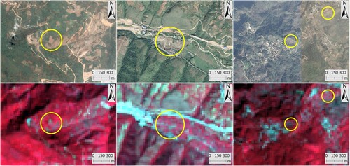
To evaluate the accuracy of fallow land detection, we employed VHR instead of field survey data (Yin et al. 2020) (Figure 3). We constructed contingency matrices between classification and validation data and conducted an accuracy assessment based on Google Earth VHR imagery; 100 sample points for each year were randomly generated for the period from 2009 to 2019. The fallow plot results were randomly selected as sample points to match the fallow cropland in the VHR. The 11-year average accuracy was used instead of the overall accuracy.

Figure 3. Examples of fallow areas in YYC, marked with yellow circles. Note: the examples in the figure were from 2019 VHR satellite images available from the Google Earth online mapping service (top: true-like visible bands) and Landsat images (bottom: near-infrared band in red; red band in green; and green band in blue false-color combinations). The images from top to bottom are the VHR images and the corresponding Landsat images.

3.3. Monitoring fallow land distribution from 2001 to 2019

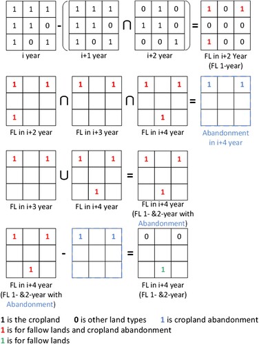
We extracted croplands from produced land cover types from 1998 to 2019 to calculate the proportions of active and fallow lands. In China, abandoned cropland is generally defined as land that has not been cultivated for 3 or more years (Han and Song 2019; Li and Song 2021; Wang and Song 2021). For our purpose, we assumed that fallow lands had not been cultivated for one or two years from 1998 to 2019, as shown in the land cover as grassland or bare land. Further, we superimposed the produced land cover maps as follows (Figure 4) (Manzungu and Mtali 2012; Srivastava et al. 2012): (1) Cropland was set to ‘1’, and the other areas were set to ‘0’; (2) cropland data for two years were superimposed. The data from the previous year minus the superimposed result was fallow land, which had been fallow for one year; (3) based on step (2), the union of three-year fallow data minus the intersection of the three-year fallow data. This limited the continuous fallow data to two years or less. With these calculations, the fallow land areas in YYC from 2001 to 2019 were obtained.

Figure 4. Identification and calculation of fallow lands.

Note: FL represents fallow lands, and ‘FL in i+2 (FL 1-year)’ signifies that it had been fallow for one year in i+2 year; ‘Abandonment in i+4 year’ represents croplands that had been fallow for three years as of i+4; ‘FL in i+4 (FL 1- &2-year with abandonment)’ represents croplands that had been fallow for one to two years as of i+4, but abandonment was not considered; ‘FL in i+4 (FL 1- &2-year)’ refers to the croplands that had been fallow for one to two years as of i+4; areas that had been fallow for more than two years were removed.

3.4. Spatial and temporal analysis of fallow lands

We evaluated the distribution of fallow lands using kernel density analysis (KD), which represents a density function that estimates unknown characteristic data. This analysis, which is a non-parametric test method, can be applied to study the distribution characteristic of data from the data sample itself, without prior knowledge of relevant data distributions (Silverman 1986). The higher the kernel density mimics the higher the spatial distribution density of fallow lands and vice versa. For this type of analysis, the fallow pixels were converted into point data in the ArcGIS 10.2 software, and the KD was then used to analyze the point data of fallow lands. Using this approach, we were able to identify the cold- and hot-spot fallow areas. The calculation formula is as follows (Silverman 1986): (2) $F_n={\displaystyle \frac{1}{nh}\sum _{i=1}^{n}k\left({\displaystyle \frac{x-x_i}{h}}\right),}$(2) where $F_n$ presents the kernel density value of the spatial distribution of fallow lands in YYC; $n$ represents the number of fallowing sites, $k$ presents the function of kernel density measurements; $x-x_i$ presents the distance between fallow plots; and $h$ presents the search radius. Since our input data were in meters, all outputs were in square kilometers (Silverman 1986). We selected 2,500 meters (Wang and Song 2021) as the radius parameter for KD calculation based on the fallow land distribution data to have a radius value not too large and too small for aggregation of fallow lands.

The linear model linked the KD results with information on topography, distance to rural settlements, and RDP data. We used the p-value < 0.05, i.e. a significance level of 95%, to determine whether the correlation was significant. Subsequently, the spatial distribution characteristics of fallow lands were analyzed. We evaluated a linear regression between the kernel density distribution with the topography and RDP data to show their effects on fallow land distribution. This was done to explore the variations in kernel density in different areas of rural settlements and determine the impacts of rural settlements on the distribution of fallow lands. The buffer of the rural settlement area was set to 10 gradients, each with a range of 1 kilometer.

4. Results

4.1. Accuracy assessment

The overall accuracy (OA) of the land cover classification results for the period 1998–2019 ranged from 90.1% (2007) to 95.8% (2012) (Table S1), with an average of 92.0% (Table 3). The highest average PA was obtained for the forest class and the highest average UA for the water class. Overall, the accuracy was sufficient for cross-validation land cover analysis.

Table 3. Average classification accuracies from 1998 to 2019. PA = producer’s accuracy; UA = user’s accuracy.

Land cover type	PA (%)	UA (%)
Cropland	95.8	88.8
Forest	96.4	96.3
Grassland	82.9	91.6
Water	81.9	98.0
Built-up	90.5	91.0
Bare land	82.7	93.5
Overall accuracy	92.0%
Kappa coefficient	89.6%

To verify the accuracy of fallow land mapping, historical images from Google for the period from 2009 to 2019 were used. Accuracy ranged from 70% to 81%, with an average of 75.7% (Table 4).

Table 4. Accuracy of fallow land mapping from 2009 to 2019.

Year	2009	2010	2011	2012	2013	2014	2015	2016	2017	2018	2019
Accuracy (%)	73.0	72.0	79.0	77.0	71.0	76.0	70.0	75.0	79.0	80.0	81.0

4.2. Interpretation results for land cover and fallow lands

4.2.1. Spatial distribution of land cover types

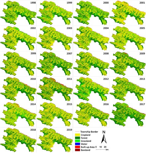
Remotely-sensed data from 1998 to 2019, composed of EVI, DEM, and Landsat data, were used to produce land-cover map for each of 22 years of observations (Figure 5). According to the results, there was a high dynamic from 1998 to 2019, with the frequent transitioning of cropland to forest. However, croplands were a common feature of the landscape in YYC, followed by forest areas and grassland. Despite the good classification accuracies, some areas were misclassified, particularly in the years with sub-optimal cloud conditions, when limited satellite observations did not allow the accurate separation of grasslands and croplands. Because the rivers in YYC were small, with large amounts of sediment, they were often confused with built-up (for more details, see Table S2).

Figure 5. Land cover maps for Yuanyang County (1998–2019).

4.2.2. Revealing fallow lands

Based on the land cover classification results, fallow data were extracted using time series overlays from cropland data. From 2001 to 2019, the annual fallow rate of YYC varied between 8.3% and 54.3%, the yearly fallow area was 286.3 km², and the fallow rate was 20.7% (Figure 6a). The temporal and spatial trends and the distribution of fallow lands were similar, including the time distribution of fallow lands in the percentage of croplands and the division of administrative regions. The fallow rate was observed at 3.4%–16.7% with high fallow rate more than 50% in 2017. Our hypothesis, this was the result of the implementation of fallow pilot program in 2017 (Lu et al. 2019). This program and the spontaneous behavior of farmers had a collective impact and led to an abnormally high fallow rate in YYC in 2017. The fallow rate in 2009 was also significant, linked to local field rehabilitation projects and the large-scale construction of irrigation facilities.

Figure 6. Fallow rate (a) and cluster analysis (b) for Yuanyang townships.

Note: The mean was set for the clustering method, Pearson’s correlation was chosen for the cluster type, and the fallow rate was used for the clustering data.

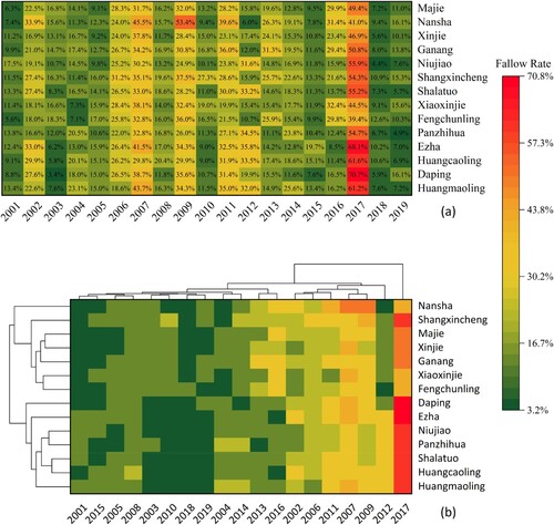
The fallow rate in YCC for 19 consecutive years indicated an obvious fallow fluctuation in the region, and the fallow rate changes were potentially cyclical (Figure 6b), such as the low fallow rate in adjacent years in 2007, 2009, 2012, and 2017. Notably, there was a cliff-like decrease in the fallow rate after 2017. Spatially, neighboring townships had similar characteristics of fallow rates (e.g. Majie and Xinjie, Niujiao and Panzhihua, Xiaoxinjie, and Fengchunlin). The phenomenon may be caused by the continuous cropland distribution in these townships, representing differences in fallow rates that transcend administrative boundaries.

4.3. Temporal-spatial distribution of fallow lands from 2001 to 2019

4.3.1. Time series analysis of the kernel density of fallow lands

The interval threshold of the natural breakpoint method was counted by mode, and the kernel density results were divided into five levels according to the natural breakpoint method. Results from a period of 11 years were used, with the upper limit of the first level around five and the lowest values ranging from 0 to 5 blocks per km². Finally, the manually adjusted kernel density classification threshold ranged from 2001 to 2019, with 0–5 blocks per km², 5–8 blocks per km², 8–13 blocks per km², 13–20 blocks per km², and above 20 blocks per km² for each of the five levels, respectively (Figure 7). The maximum kernel density of fallow lands in YYC was 50 blocks per km² (2015), and the overall peak performance fluctuated around 35 blocks per km². From the perspective of the grade distribution of each year, the years with more than 20 blocks per km² accounted for approximately one-third of the statistical years; 13–20 blocks per km² were widely distributed in 2001, 2008, 2011–2014, and 2018. The years when the kernel density value was 8–13 blocks/km² were 2008 and 2012. The distribution of kernel density values of 5–8 blocks per km² was not obvious in many years and was mainly found for 2007–2011. The value was most widely distributed between 0- and 5 blocks per km².

Figure 7. Spatial distribution of kernel density of fallow lands in Yuanyang (2001–2019).

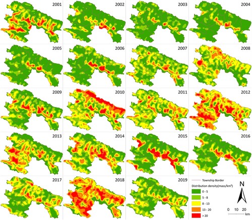
We noticed, once the national fallow program was officially launched in China in 2017, that the fallow land in YYC increased in 2018. We also observed the same case with high fallow rates in 2012. We speculate that the brief but concentrated stagnation in farming (temporary fallowing) was caused by a large outmigration of the agricultural population (Han and Song 2019).

4.3.2. Topographic statistics of the temporal and spatial distribution of fallow lands

The mean KD results and DEM data were superimposed and analyzed to explore the influences of terrain factors on the KD distribution of fallow lands. KD ratings increased with increased elevation (Table 5). High-areas have generally poor soil quality and moisture (Yang et al. 2022), resulting in an increase in the fallow frequency. Also, the soil at high elevations is unsuitable for continuous cultivation. Also, in YYC, at elevation above 2,500 m, agriculture is not feasible. The linear fit between the KD rank and the elevation minimum, maximum, and mean were 0.811, 0.832, and 0.950 (p-value < 0.05), respectively (Figure 8), showing a significant linear relationship between fallow KD grade and elevation.

Figure 8. Relationships between KD rating and elevation of fallow land areas.

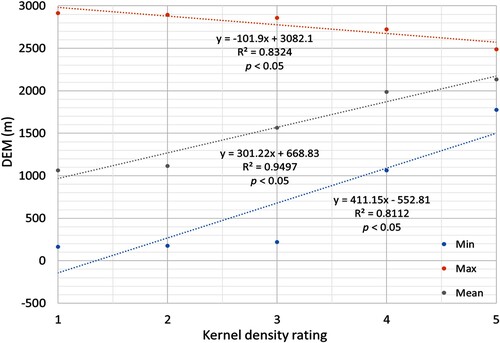
Table 5. Statistics on kernel density (KD) distribution and elevation of fallow land area.

KD rating	KD value (km^2)	Elevation
		Minimum value	Maximum value	Mean
1	0–5	166	2,914	1,064
2	5–8	177	2,896	1,114
3	8–13	218	2,858	1,565
4	13–20	1,065	2,725	1,987
5	>20	1,777	2,489	2,132

4.3.3. RDP statistics versus temporal and spatial distribution of fallow lands

The average level of KD was used in the statistical calculations of the RDP. The spatial distribution of the KD of fallow was closely related to the maximum and minimum values of the RDP. The linear regression R² values were 0.876 and 0.847 (max. and min.), and the mean R² was less than 0.5 at a significance level of 95% (Table 6). With the increase in the kernel density rate of fallow lands, the RDP decreased from 4.88 to 1.19 million yuan/km². In contrast, the minimum RDP value increased from 490,000 to 750,000 yuan/km². According to the statistics of the spatial distribution of the RDP, the spatial distribution of the KD of fallow was strongly correlated with the RDP. With the increase in fallow KD, the maximum RDP value showed a decreasing trend, and the minimum value showed an increasing trend.

Table 6. Statistics on RDP distribution versus fallow land areas.

KD rating	KD value (km^2)	RDP
		Minimum value	Maximum value	Mean
1	0–5	49	488	92
2	5–8	45	345	82
3	8–13	53	171	80
4	13–20	70	120	83
5	>20	75	119	90

4.3.4. Rural settlement statistics of the temporal and spatial distribution of fallow land areas

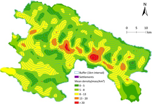
The spatial distribution of the average results of the KD of settlements in fallow land areas was calculated, and the impacts of rural settlements on fallow land areas were explored (Figure 9). A large amount of dense fallow land could be identified around rural settlements. The settlements of YYC covered an area of 2.9 km², with 15.4% of the area having a rating range from 0 to 5 blocks per km², 49.8% with 5–8 blocks per km², and 31.8% with 8–13 blocks per km². Only 3.0% of rural settlements had more than 13 blocks per km²; the area is characterized by roads and trees around the rural settlements, with a small stock of cropland (Chen et al. 2022).

Figure 9. The spatial relationship between rural settlements and fallow land kernel density.

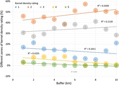
By further analyzing the buffer (Figure 10), as croplands moved away from the rural settlement, the KD rate of fallowing showed a downward trend, i.e. the density of fallow lands decreased with increasing distance from the rural settlements. In areas far from rural settlements, kernel density ranks 2 (5–8 blocks per km²) and 3 (8–13 blocks per km²) showed an upward trend, whilst ranks 1, 4, and 5 revealed a downward trend. In particular, the area with a high KD of fallow land, i.e. the area with ratings 4 and 5 (p-value < 0.05), was significantly correlated with the distance from the settlement. This shows that in mountainous areas, cropland is mainly distributed near settlements (Liang and Li 2020).

Figure 10. Multi-gradient buffer kernel density rating.

5. Discussion

5.1. Extent of the fallow area and its temporal trend

In our study, fallow lands accounted for approximately one-fifth of the cropland areas in YYC, with a low fallow rate. In a previous study, fallow land accounted for 13.7% of the cropland in Youyang County (Chongqing, China) (Song 2019), whereas the average fallow rate in Europe is about 24.43% (Estel et al. 2015), that in the northern mountainous areas of Laos is 65.3% (Yamamoto, Oberthür, and Lefroy 2009), and that in the Assam State of India is as high as 76.0% (Mondal et al. 2016). This indicates that the fallow rate of YYC is below the level required for natural replenishment.

The KD of fallow lands in YYC constantly changed over the years, but the kernel density values of various regions showed a certain continuity. For example, from 2002 to 2006, the five ratings of kernel density were similar, and the kernel density ratings in the northeast, southeast, and southwest of YYC were lower than those in other regions. However, over the past 10 years, the kernel density ratings gradually increased, especially regarding the distribution of areas with more than eight blocks per km², indicating that the number of fallow fields had become concentrated or increased.

5.2. Association of selected factors and fallow land

We used the three factors that may determine the spatial distribution of fallow land: elevation, RDP, and distance to rural settlements. According to the correlation between topography and the temporal and spatial distribution of fallow land, elevation significantly influenced the spatial distribution of fallow land (R² from 0.811to 0.950). The higher the elevation, the higher the number of fallow fields. Other studies (Yamamoto, Oberthür, and Lefroy 2009; Song 2019) support the strong relationship between elevation and fallow, and it can be concluded that topographical elements are indispensable when identifying fallow land and studying its temporal and spatial characteristics.

In this study, the correlation between RDP and fallow was mainly reflected in the aspect of economic viability, showing that fallowing is strongly related to the economic performance of the region (Wang, Siriwardana, and Meng 2019; Xie and Jin 2019). We used superimposed statistics on the spatial distribution of RDP and the nuclear density of fallow lands, which exhibited a negative relationship.

Over 65% of the area fell into the first two kernel density ratings, indicating that fallow cropland in YYC was not concentrated. As the distance from the settlement increased, fallow fields became more dispersed (KD rating = 5, R² = 0.725, p-value < 0.05; KD rating = 4, R²= 0.426, p-value < 0.05), clearly showing that rural settlements interfere with fallowing. Studies of areas other than areas of residence would also derive the same or similar conclusions (Song 2019), and we therefore assume that the occurrence of fallowing is largely related to the spontaneous behavior of farmers (Xie and Jin 2019).

5.3. Policies and future studies

Our results have two main implications for fallow policies. First, we observed a clear increase of fallowing with increasing elevation. Fallow lands may partially show early signs of cropland abandonment. As mountainous areas are prone to farmland abandonment (Han and Song 2019; Song 2019), regional authorities should focus on such regions. Second, the government may strengthen communication with farmers to curtail spontaneous fallowing. The Chinese government implemented a unified fallow work from 2017 (Ministry of Agriculture and Rural Affairs of the People’s Republic of China 2017), which further improved the government’s ability to regulate fallow land.

We studied the relationship between fallowing patterns and elevation, RDP, and distances to settlements. Future studies may use a ‘bottom-up’ approach, revealing the influences of personal factors of farmers in connection to fallowing. Moreover, from the perspective of food security and cropland sustainability, we will further explore the impacts of water availability on fallow, as well as the impacts of fallow on food prices and grain production. The advent of frequent observations at high spatial resolutions, such as via Planet scope, opens up a great opportunity to nuance cultivated and fallow patterns in parceled farming areas, such as in mountainous regions of China.

6. Conclusions

We mapped fallow cropland in Yuanyang County, Yunnan Province, China, from 2001 to 2019 by reconstructing annual land cover data from 1998 to 2019. Kernel density analysis was employed to investigate the temporal–spatial distribution and the factors influencing fallow land. The average OA and Kappa coefficient values of land cover were 92.0% and 89.6%, respectively. The annual fallow rate was 20.7%, ranging from 8.30% to 54.3%. The accuracy of fallow land recognition was 75.7%. In the temporal–spatial distribution, the kernel density of fallow land in YYC was 5–13 blocks per km². Kernel density was higher at higher elevations. The density of fallow lands decreased with increasing distance from the rural settlements. The method developed here can be applied to various areas and regions.

CRediT authorship contribution statement

Wen Song: Formal analysis, Methodology, Writing original draft, Writing review & editing. Alexander V Prishchepov: Methodology, Writing review & editing. Wei Song: Conceptualization, Data curation, Resources, Methodology, Funding acquisition, Writing review & editing.

Data availability

The data that support the findings of this study (i.e. the land cover and fallow land maps) are available from the corresponding author, Wei Song, upon reasonable request.

Disclosure statement

No potential conflict of interest was reported by the author(s).

Additional information

Funding

This research was supported by the National Natural Science Foundation of China [grant number 42071233], the Strategic Priority Research Program of Chinese Academy of Sciences [grant number XDA20040201], and the Second Tibetan Plateau Scientific Expedition and Research Program [grant number 2019QZKK0603].

References

- Babu, Subhash, K. P. Mohapatra, Anup Das, Gulab Singh Yadav, Moutusi Tahasildar, Raghavendra Singh, A. S. Panwar, Vivek Yadav, and Puran Chandra. 2020. “Designing Energy-Efficient, Economically Sustainable and Environmentally Safe Cropping System for the Rainfed Maize–Fallow Land of the Eastern Himalayas.” Science of The Total Environment 722: 137874. doi:10.1016/j.scitotenv.2020.137874.
- Belgiu, Mariana, and Lucian Drăguţ. 2016. “Random Forest in Remote Sensing: A Review of Applications and Future Directions.” ISPRS Journal of Photogrammetry and Remote Sensing 114: 24–31. doi:10.1016/j.isprsjprs.2016.01.011.
- Brinson, Mark M., and S. Diane Eckles. 2011. “U.S. Department of Agriculture Conservation Program and Practice Effects on Wetland Ecosystem Services: A Synthesis.” Ecological Applications 21 (sp1): S116–S127. doi:10.1890/09-0627.1.
- Chandna, Parvesh Kumar, and Saptarshi Mondal. 2020. “Analyzing Multi-Year Rice-Fallow Dynamics in Odisha Using Multi-Temporal Landsat-8 OLI and Sentinel-1 Data.” GIScience & Remote Sensing 57 (4): 431–449. doi:10.1080/15481603.2020.1731074.
- Chen, Jun, Jin Chen, Anping Liao, Xin Cao, Lijun Chen, Xuehong Chen, Chaoying He, et al. 2015. “Global Land Cover Mapping at 30m Resolution: A POK-Based Operational Approach.” ISPRS Journal of Photogrammetry and Remote Sensing 103: 7–27. doi:10.1016/j.isprsjprs.2014.09.002.
- Chen, Hongji, Kangchuan Su, Lixian Peng, Guohua Bi, Lulu Zhou, and Qingyuan Yang. 2022. “Mixed Land Use Levels in Rural Settlements and Their Influencing Factors: A Case Study of Pingba Village in Chongqing, China.” International Journal of Environmental Research and Public Health 19 (10): 5845. doi:10.3390/ijerph19105845.
- Chengming, Zhang, Liu Jiping, Yu Fan, Wan Shujing, Han Yingjuan, Wang Jing, and Wang Gang. 2018. “Segmentation Model Based on Convolutional Neural Networks for Extracting Vegetation from Gaofen-2 Images.” Journal of Applied Remote Sensing 12 (4): 1–18. doi: 10.1117/1.JRS.12.042804.
- Conrad, Christopher, Stefan Dech, Olena Dubovyk, Sebastian Fritsch, Doris Klein, Fabian Löw, Gunther Schorcht, and Julian Zeidler. 2014. “Derivation of Temporal Windows for Accurate Crop Discrimination in Heterogeneous Croplands of Uzbekistan Using Multitemporal RapidEye Images.” Computers and Electronics in Agriculture 103: 63–74. doi:10.1016/j.compag.2014.02.003.
- Estel, Stephan, Tobias Kuemmerle, Camilo Alcántara, Christian Levers, Alexander Prishchepov, and Patrick Hostert. 2015. “Mapping Farmland Abandonment and Recultivation Across Europe Using MODIS NDVI Time Series.” Remote Sensing of Environment 163: 312–325. doi:10.1016/j.rse.2015.03.028.
- Felde, Gerald W., Gail P. Anderson, Thomas W. Cooley, Michael W. Matthew, Steven M. Adler-Golden, Alexander Berk, and Jamie Lee. 2003. “Analysis of Hyperion Data with the FLAASH Atmospheric Correction Algorithm.” IGARSS 2003. 2003 IEEE International Geoscience and Remote Sensing Symposium. Proceedings (IEEE Cat. No.03CH37477), July 21–25.
- Girard, C. M., C. Le Bas, W. Szujecka, and M. C. Girard. 1994. “Remote Sensing and Fallow Land.” Journal of Environmental Management 41 (1): 27–38. doi:10.1006/jema.1994.1031.
- Gong, Peng, Han Liu, Meinan Zhang, Congcong Li, Jie Wang, Huabing Huang, Nicholas Clinton, et al. 2019. “Stable Classification with Limited Sample: Transferring a 30-m Resolution Sample Set Collected in 2015 to Mapping 10-m Resolution Global Land Cover in 2017.” Science Bulletin 64 (6): 370–373. doi:10.1016/j.scib.2019.03.002.
- Groier, M. 2000. “The Development, Effects and Prospects for Agricultural Environmental Policy in Europe.” Förderungsdienst 48 (4): 37–40.
- Gumma, Murali Krishna, Prasad S. Thenkabail, Kumara Charyulu Deevi, Irshad A. Mohammed, Pardhasaradhi Teluguntla, Adam Oliphant, Jun Xiong, Tin Aye, and Anthony M. Whitbread. 2018. “Mapping Cropland Fallow Areas in Myanmar to Scale Up Sustainable Intensification of Pulse Crops in the Farming System.” GIScience & Remote Sensing 55 (6): 926–949. doi:10.1080/15481603.2018.1482855.
- Han, Ze, and Wei Song. 2019. “Spatiotemporal Variations in Cropland Abandonment in the Guizhou–Guangxi Karst Mountain Area, China.” Journal of Cleaner Production 238: 117888. doi:10.1016/j.jclepro.2019.117888.
- Li, Han, and Wei Song. 2021. “Cropland Abandonment and Influencing Factors in Chongqing, China.” Land 10 (11): 1206. doi:10.3390/land10111206.
- Liang, Xinyuan, and Yangbing Li. 2020. “Identification of Spatial Coupling Between Cultivated Land Functional Transformation and Settlements in Three Gorges Reservoir Area, China.” Habitat International 104: 102236. doi:10.1016/j.habitatint.2020.102236.
- Liu, Luo, Xinliang Xu, Dafang Zhuang, Xi Chen, and Shuang Li. 2013. “Changes in the Potential Multiple Cropping System in Response to Climate Change in China from 1960-2010.” PloS one 8 (12): e80990. doi:10.1371/journal.pone.0080990.
- Lu, Dan, Yahui Wang, Qingyuan Yang, Huiyan He, and Kangchuan Su. 2019. “Exploring a Moderate Fallow Scale of Cultivated Land in China from the Perspective of Food Security.” International Journal of Environmental Research and Public Health 16 (22): 4329. doi:10.3390/ijerph16224329.
- Manzungu, Emmanuel, and Linda Mtali. 2012. “An Investigation Into the Spatial and Temporal Distribution of Fallow Land and the Underlying Causes in Southcentral Zimbabwe.” Journal of Geography and Geology 4 (4): 62. doi:10.5539/jgg.v4n4p62.
- Masek, J. G., E. F. Vermote, N. E. Saleous, R. Wolfe, F. G. Hall, K. F. Huemmrich, Gao Feng, J. Kutler, and Lim Teng-Kui. 2006. “A Landsat Surface Reflectance Dataset for North America, 1990-2000.” IEEE Geoscience and Remote Sensing Letters 3 (1): 68–72. doi:10.1109/LGRS.2005.857030.
- Ministry of Agriculture and Rural Affairs of the People's Republic of China. 2017. “Notice of the Ministry of Agriculture and the Ministry of Finance on the Implementation of Projects Such as the Development of Agricultural Production in the Central Government in 2017.” Accessed January 10, 2021. http://www.moa.gov.cn/.
- Mondal, Md Surabuddin, Nayan Sharma, P. K. Garg, and Martin Kappas. 2016. “Statistical Independence Test and Validation of CA Markov Land use Land Cover (LULC) Prediction Results.” The Egyptian Journal of Remote Sensing and Space Science 19 (2): 259–272. doi:10.1016/j.ejrs.2016.08.001.
- Nguyen, Can T., Amnat Chidthaisong, Phan Kieu Diem, and Lian-Zhi Huo. 2021. “A Modified Bare Soil Index to Identify Bare Land Features During Agricultural Fallow-Period in Southeast Asia Using Landsat 8.” Land 10 (3): 231. doi:10.3390/land10030231.
- Phalke, Aparna R., and Mutlu Özdoğan. 2018. “Large Area Cropland Extent Mapping with Landsat Data and a Generalized Classifier.” Remote Sensing of Environment 219: 180–195. doi:10.1016/j.rse.2018.09.025.
- Prosekov, Alexander Y., and Svetlana A. Ivanova. 2018. “Food Security: The Challenge of the Present.” Geoforum; Journal of Physical, Human, and Regional Geosciences 91: 73–77. doi:10.1016/j.geoforum.2018.02.030.
- Rahman, Md, and S. Saha. 2009. “Spatial Dynamics of Cropland and Cropping Pattern Change Analysis Using Landsat TM and IRS P6 LISS III Satellite Images with GIS.” Geo-spatial Information Science 12 (2): 123–134. doi:10.1007/s11806-009-0249-2.
- Ram, Balak, and A. S. Kolarkar. 1993. “Remote Sensing Application in Monitoring Land-use Changes in Arid Rajasthan.” International Journal of Remote Sensing 14 (17): 3191–3200. doi:10.1080/01431169308904433.
- Rasul, Azad, Heiko Balzter, Gaylan R. Faqe Ibrahim, Hasan M. Hameed, James Wheeler, Bashir Adamu, Sa’ad Ibrahim, and Peshawa M. Najmaddin. 2018. “Applying Built-Up and Bare-Soil Indices from Landsat 8 to Cities in Dry Climates.” Land 7 (3): 81. doi:10.3390/land7030081.
- Sato, Hitoshi. 2001. “The Current State of Paddy Agriculture in Japan.” Irrigation and Drainage 50 (2): 91–99. doi:10.1002/ird.10.
- Shi, Kaifang, Qingyuan Yang, Yuanqing Li, and Xiufeng Sun. 2019. “Mapping and Evaluating Cultivated Land Fallow in Southwest China Using Multisource Data.” Science of The Total Environment 654: 987–999. doi:10.1016/j.scitotenv.2018.11.172.
- Siachalou, S., G. Mallinis, and M. Tsakiri-Strati. 2017. “Analysis of Time-Series Spectral Index Data to Enhance Crop Identification Over a Mediterranean Rural Landscape.” IEEE Geoscience and Remote Sensing Letters 14 (9): 1508–1512. doi:10.1109/LGRS.2017.2719124.
- Silverman, Bernard W. 1986. Density Estimation For Statistics And Data Analysis. New York: Chapman and Hall.
- Song, Wei. 2019. “Mapping Cropland Abandonment in Mountainous Areas Using an Annual Land-Use Trajectory Approach.” Sustainability 11 (21): 5951. doi:10.3390/su11215951.
- Song, Wei, and Xiangzheng Deng. 2017. “Land-use/land-cover Change and Ecosystem Service Provision in China.” Science of The Total Environment 576: 705–719. doi:10.1016/j.scitotenv.2016.07.078.
- Song, Wei, and Bryan C. Pijanowski. 2014. “The Effects of China's Cultivated Land Balance Program on Potential Land Productivity at a National Scale.” Applied Geography 46: 158–170. doi:10.1016/j.apgeog.2013.11.009.
- Srivastava, Amit Kumar, Thomas Gaiser, Denis Cornet, and Frank Ewert. 2012. “Estimation of Effective Fallow Availability for the Prediction of yam Productivity at the Regional Scale Using Model-Based Multiple Scenario Analysis.” Field Crops Research 131: 32–39. doi:10.1016/j.fcr.2012.01.012.
- Styger, Erika, Harivelo M. Rakotondramasy, Max J. Pfeffer, Erick C. M. Fernandes, and David M. Bates. 2007. “Influence of Slash-and-Burn Farming Practices on Fallow Succession and Land Degradation in the Rainforest Region of Madagascar.” Agriculture, Ecosystems & Environment 119 (3): 257–269. doi:10.1016/j.agee.2006.07.012.
- Sullivan, Patrick, Daniel Hellerstein, Leroy Hansen, Robert Johansson, Steven Koenig, Ruben N. Lubowski, William D. McBride, David A. McGranahan, Michael J. Roberts, and Stephen J. Vogel. 2004. “The Conservation Reserve Program: Economic Implications for Rural America.” USDA-ERS Agricultural Economic Report 834: 112. doi:10.2139/ssrn.614511.
- Van der Linden, Sebastian, Andreas Rabe, Matthias Held, Benjamin Jakimow, J. Pedro Leitão, Akpona Okujeni, Marcel Schwieder, Stefan Suess, and Patrick Hostert. 2015. “The EnMAP-Box—A Toolbox and Application Programming Interface for EnMAP Data Processing.” Remote Sensing 7 (9): 11249–11266. doi:10.3390/rs70911249.
- van Vliet, Nathalie, Ole Mertz, Andreas Heinimann, Tobias Langanke, Unai Pascual, Birgit Schmook, Cristina Adams, et al. 2012. “Trends, Drivers and Impacts of Changes in Swidden Cultivation in Tropical Forest-Agriculture Frontiers: A Global Assessment.” Global Environmental Change 22 (2): 418–429. doi:10.1016/j.gloenvcha.2011.10.009.
- Vermote, Eric, Chris Justice, Martin Claverie, and Belen Franch. 2016. “Preliminary Analysis of the Performance of the Landsat 8/OLI Land Surface Reflectance Product.” Remote Sensing of Environment 185: 46–56. doi:10.1016/j.rse.2016.04.008.
- Wang, Fengjiao, Wei Liang, Bojie Fu, Zhao Jin, Jianwu Yan, Weibin Zhang, Shuyi Fu, and Nana Yan. 2020. “Changes of Cropland Evapotranspiration and its Driving Factors on the Loess Plateau of China.” Science of The Total Environment 728: 138582. doi:10.1016/j.scitotenv.2020.138582.
- Wang, Can, Mahinda Siriwardana, and Samuel Meng. 2019. “Effects of the Chinese Arable Land Fallow System and Land-use Change on Agricultural Production and on the Economy.” Economic Modelling 79: 186–197. doi:10.1016/j.econmod.2018.10.012.
- Wang, Yanwei, and Wei Song. 2021. “Mapping Abandoned Cropland Changes in the Hilly and Gully Region of the Loess Plateau in China.” Land 10 (12): 1341. doi:10.3390/land10121341.
- Wu, Qing, and Hualin Xie. 2017. “A Review and Implication of Land Fallow System Research.” Journal of Resources and Ecology 8 (3): 223–231. doi:10.5814/j.issn.1674-764x.2017.03.002.
- Xie, Hualin, and Shengtian Jin. 2019. “Evolutionary Game Analysis of Fallow Farmland Behaviors of Different Types of Farmers and Local Governments.” Land Use Policy 88: 104122. doi:10.1016/j.landusepol.2019.104122.
- Xu, Xinliang. 2017. “China GDP Spatial Distribution Kilometer Grid Data Set.” Data Registration and Publishing System of Resources and Environmental Sciences Data Center, Chinese Academy of Sciences.
- Xu, X. L., J. Y. Liu, S. W. Zhang, R. D. Li, C. Z. Yan, and S. X. Wu. 2018. “Remote Sensing Monitoring Data Set for Land Use and Cover Change in China (CNLUCC).” Data Registration and Publishing System of Resource and Environment Science Data Center of Chinese Academy of Sciences. http://www.resdc.cn. doi:10.12078/2018070201.
- Yamamoto, Yukiyo, Thomas Oberthür, and Rod Lefroy. 2009. “Spatial Identification by Satellite Imagery of the Crop–Fallow Rotation Cycle in Northern Laos.” Environment, Development and Sustainability 11 (3): 639–654. doi:10.1007/s10668-007-9134-z.
- Yang, Shanshan, Jiahua Zhang, Jingwen Wang, Sha Zhang, Yun Bai, Siqi Shi, and Dan Cao. 2022. “Spatiotemporal Variations of Water Productivity for Cropland and Driving Factors Over China During 2001–2015.” Agricultural Water Management 262: 107328. doi:10.1016/j.agwat.2021.107328.
- Yin, He, Amintas Brandão, Johanna Buchner, David Helmers, Benjamin G. Iuliano, Niwaeli E. Kimambo, Katarzyna E. Lewińska, et al. 2020. “Monitoring Cropland Abandonment with Landsat Time Series.” Remote Sensing of Environment 246: 111873. doi:10.1016/j.rse.2020.111873.
- Yuanyang County People’s Government Office. 2020. “1989-2019 Yuanyang County Statistical Yearbook.” Accessed January 3, 2020. http://www.yy.hh.gov.cn/.
- Zambon, Ilaria, Pere Serra, Rosanna Salvia, and Luca Salvati. 2018. “Fallow Land, Recession and Socio-Demographic Local Contexts: Recent Dynamics in a Mediterranean Urban Fringe.” Agriculture 8 (10): 159. doi:10.3390/agriculture8100159.
- Zhang, Ying, Xiubin Li, and Wei Song. 2014. “Determinants of Cropland Abandonment at the Parcel, Household and Village Levels in Mountain Areas of China: A Multi-Level Analysis.” Land Use Policy 41: 186–192. doi:10.1016/j.landusepol.2014.05.011.
- Zhang, Xiaomei, Tengfei Long, Guojin He, and Yantao Guo. 2019. “Gobal Forest Cover Mapping Using Landsat and Google Earth Engine Cloud Computing.” 2019 8th International Conference on Agro-Geoinformatics (Agro-Geoinformatics), July 16–19.
- Zhong, Y., C. Giri, P. S. Thenkabail, P. Teluguntla, G. Congalton, R. K. Yadav, J. A. Oliphant, J. Xiong, J. Poehnelt, and C. Smith. 2017. “NASA Making Earth System Data Records for Use in Research Environments (MEaSUREs) Global Food Security-support Analysis Data (GFSAD) Cropland Extent 2015 South America 30 m V001.” Edited by NASA EOSDIS Land Processes DAAC. NASA EOSDIS Land Processes DAAC.
- Zhu, Zhe, Shixiong Wang, and Curtis E. Woodcock. 2015. “Improvement and Expansion of the Fmask Algorithm: Cloud, Cloud Shadow, and Snow Detection for Landsats 4–7, 8, and Sentinel 2 Images.” Remote Sensing of Environment 159: 269–277. doi:10.1016/j.rse.2014.12.014.