Spatiotemporal variations in surface albedo during the ablation season and linkages with the annual mass balance on Muz Taw Glacier, Altai Mountains

ABSTRACT

Melt-albedo feedback on glaciers is recognized as important processes for understanding glacier behavior and its sensitivity to climate change. This study selected the Muz Taw Glacier in the Altai Mountains to investigate the spatiotemporal variations in albedo and their linkages with mass balance, which will improve our knowledge of the recent acceleration of regional glacier shrinkage. Based on the Landsat-derived albedo, the spatial distribution of ablation-period albedo was characterized by a general increase with elevation, and significant east–west differences at the same elevation. The gap-filling MODIS values captured a nonsignificant negative trend of mean ablation-period albedo since 2000, with a total decrease of approximately 4.2%. From May to September, glacier-wide albedo exhibited pronounced V-shaped seasonal variability. A significant decrease in annual minimum albedo was found from 2000 to 2021, with the rate of approximately −0.30% yr⁻¹ at the 99% confidence level. The bivariate relationship demonstrated that the change of ablation-period albedo explained 82% of the annual mass-balance variability. We applied the albedo method to estimate annual mass balance over the period 2000–2015. Combined with observed values, the average mass balance was −0.82 ± 0.32 m w.e. yr⁻¹ between 2000 and 2020, with accelerated mass loss.

KEYWORDS:

• Albedo
• spatiotemporal variation
• glacier mass balance
• remote sensing
• Altai Mountains

1. Introduction

Mountain glaciers are recognized as a sensitive and high-confidence climate indicator (Roe, Baker, and Herla 2017; Yang et al. 2019). Moreover, mountain glaciers are important water resources at the headwaters of many prominent rivers (Lu et al. 2020; Chen et al. 2022), which impact the downstream water availability and sea level rise (Huss and Hock 2018; Zemp et al. 2019) and potentially influence natural hazards (Zheng et al. 2021). Glacier mass balance is a direct and immediate response to climate conditions (Zemp, Hoelzle, and Haeberli 2009). Net shortwave radiation contributes predominantly energy to glacier melting (Hock and Holmgren 2005; Gurgiser et al. 2013; Schaefer et al. 2020). Albedo, defined as the ratio of the outgoing radiant flux reflected from the Earth’s surface to the total incoming flux over the whole solar spectrum (Shuai et al. 2020), modulates the quantity of net shortwave radiation. Therefore, albedo is one of the key driving factors governing the surface mass-balance conditions of mountain glaciers. Glacier mass balance and its sensitivity to climate change depend to a large degree on the albedo and albedo feedback (Klok and Oerlemans 2004).

The decline over time of ice/snow albedo, which appears as surface darkening, has been found by in-situ measurements, remote sensing techniques, or modeling approaches for worldwide ice sheets and glaciers, e.g. in Greenland (Alexander et al. 2014), European Alps (Oerlemans, Giesen, and Van Den Broeke 2009), Tibetan Plateau and its surrounding areas (Zhang et al. 2021). The decrease in surface albedo has been linked to abnormal warming at high latitudes (Box et al. 2012). For glaciers in low and middle latitudes, the positive albedo-feedback mechanism is primarily responsible for accelerating mass loss (Johnson and Rupper 2020). On remote and relatively inaccessible glaciers, the albedo method was proposed to reconstruct the glacier-wide annual surface mass balance, based on the strong correlation between the summer glacier-wide averaged albedo and the annual surface mass balance (Dumont et al. 2012); this approach has been widely applied and validated in different regions (e.g. Brun et al. 2015; Sirguey et al. 2016; Zhang et al. 2018).

In the Altai Mountains and surroundings, glaciers cover a total of about 1191 km² (Randolph Glacier Inventory 2017). These glaciers are an important source of freshwater for the upper tributaries of many prominent North Asian rivers, such as the Ob, Irtysh, and Yenisei rivers. Satellite measurements and model simulations indicate that the Altai Mountains glaciers have undergone significant, accelerated mass losses over past decades (e.g. Kadota and Gombo 2007; Surazakov et al. 2007; Shahgedanova et al. 2010; Zhang et al. 2017; Chang et al. 2022; Su et al. 2022). So far, the reasons for the accelerated glacier shrinkage in the Altai Mountains fall into two consensuses. (1) Glacier wastage is mainly attributed to the increase in air temperature (Zhang et al. 2017; Chang et al. 2022). (2) Spatial heterogeneities in precipitation probably contribute to the subregion differences in glacier wastage (Wei et al. 2015; Zhang et al. 2017).

However, multiproxy studies have demonstrated that warming climate can induce a series of complex variations in glacier surface processes, including the enhancement of snow metamorphic rate, increasing water content at the glacier surface, the expansion of bare ice areas, and prolonged exposure of bare ice (Box et al. 2012). These variations in surface processes trigger positive melt–albedo feedback, decreasing surface albedo, and further accelerating melt (Johnson and Rupper 2020). Meanwhile, the warming climate is likely to cause changes in precipitation form, especially in summer; decreasing the snowfall frequency will reduce the mean ablation-period albedo (Klok and Oerlemans 2004). The reduction of mean albedo, together with heat flux supplied by rainfall, accelerates glacier melting. Thus, albedo and its feedback process will amplify the impact of climate warming on glacier melting (Naegeli and Huss 2017). Johnson and Rupper (2020) stated that up to 80% of the average glacier melt increase, from a + 1°C temperature rise, can be attributed to albedo feedback. In addition, increased ablation accelerates the accumulation of subglacial impurities on the glacier surface, which also contributes to albedo decline (Tedesco et al. 2016). Driven by these feedback mechanisms, little is known about the variations in surface albedo of Altai Mountains glaciers (Wang et al. 2014; Zhang et al. 2021). The contribution of albedo changes to glacier shrinkage also remains to be quantitatively assessed.

Field-based measurements provide information about the surface albedo at specific locations, with limited spatial extent but high temporal resolution. Remote sensing methods enable monitoring of the surface albedo at large spatial scales, but are limited to the times of clear-sky overpasses. Modeling approaches break through the limitations of spatial and temporal resolution, but the rugged mountainous terrain challenges the simulation accuracy. Meanwhile, most models lack a module associated with the presence of light-absorbing impurities (Tedesco et al. 2016).

Here, we combine satellite-derived and field-observed data to investigate the spatiotemporal evolution of surface albedo and its linkages with the annual mass balance. Muz Taw Glacier, situated in the southern Altai Mountains was selected for this study. Since 2013, systematic glaciological observations on the Muz Taw Glacier have been carried out by an observation and research station, including meteorology, mass balance, thickness, surface topography, surface albedo, and light-absorbing impurities. These field observations validate satellite-derived albedo measurements, and provide a data set for studying the influence of albedo on mass balance. Given the fact that the available glaciological data series are sparse and most of them were discontinued in the Altai Mountains in the latter decades of the twentieth century, this study helps to improve our understanding of glacier behavior in the region since 2000.

2. Study area

The Muz Taw Glacier (47°04′N, 85°34′E), located in the interior of the Eurasian continent, is a typical valley glacier (Figure 1a and c). The glacier is exposed to the northeast, covers an area of 3.04 km², and extends from an altitude of 3150 m above sea level (a.s.l.) to 3825 m a.s.l. (Figure 1b). Here, using a Landsat 8 image acquired in July 2015, the glacier outline was manually mapped, with the expected uncertainties of ±5% of the total glacier area for medium-resolution images (Paul et al. 2013). The glacier outline remained constant in subsequent studies.

Figure 1. (a) Geographical location and (b) map of Muz Taw Glacier. The elevation contours were extracted from the Advanced Spaceborne Thermal Emission and Reflection Radiometer Global Digital Elevation Model Version 3 (ASTER GDEM v3) (http://earthexplorer.usgs.gov). The Moderate Resolution Imaging Spectroradiometer (MODIS) albedo image (date: August 14, 2018) from the National Snow and Ice Data Center (https://modis.gsfc.nasa.gov/data/dataprod/mod10.php) is shown with crosses representing the pixels selected to calculate glacier-wide albedo. (c) Landscape photograph of Muz Taw Glacier and (d) a photograph of the on-glacier automatic weather station (AWS) are also shown, which were taken on August 14, 2018.

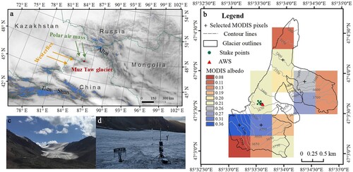
Geophysical surveys in 2013 revealed a maximum ice thickness of 122 m at the location near the main flow line of the glacier at approximately 3360 m a.s.l., and an average thickness of 60.5 m (Huai et al. 2015). The mean ice flow velocity ranged from 0.11 m a⁻¹ to 0.86 m a⁻¹ between 3100 m a.s.l. and 3300 m a.s.l. (Xu et al. 2021). Over the past 40 years (1977–2017), the glacier has experienced a rapid and accelerated shrinkage, with a reduction 45.72% of its total area, and a mean length change of 11.5 m yr⁻¹ (Wang et al. 2019).

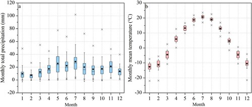
The general circulation over the study area features the prevailing westerlies, interacting with the Siberian high and polar air mass in winter (Panagiotopoulos et al. 2005). This area is characterized by strong seasonality in air temperature and relatively low seasonality in precipitation (Figure 2). Mean annual air temperature is approximately 1.2°C–6.3°C (mean: 4.3°C) and annual precipitation is generally 110–364 mm (mean: 212 mm) based on records for 1961–2016 at the Jimunai Meteorological Station (984 m a.s.l.), 46-km northeast of the Muz Taw Glacier. Meteorological observations indicate that the Sawir Mountains have experienced significant warming and wetting since 1961, with increase rates of 0.4°C (10 yr)⁻¹ for air temperature and 12 mm (10 yr)⁻¹ for precipitation.

Figure 2. (a) Monthly total precipitation and (b) mean air temperature recorded by Jimunai Meteorological Station (located 46-km northeast of the Muz Taw Glacier at 984 m a.s.l.) between 1961 and 2016. Boxes indicate the interquartile ranges of 56 monthly values. Whiskers represent one standard deviation around the monthly mean. The median, mean, and maximum/minimum values for individual months are shown with the short horizontal line, dot, and crosses, respectively.

3. Data and methods

3.1. Satellite albedo data

3.1.1. MODIS albedo product

The Moderate Resolution Imaging Spectroradiometer (MODIS) MOD10A1-V061 and MYD10A1-V061 snow products (tile: h23v04), generated by the National Snow and Ice Data Center, were applied to inquire into surface albedo temporal variations. These snow products provide daily blue-sky albedo, snow cover, and corresponding quality assessments with 500-m spatial resolution at the satellite platform overpass (at approximately 10:30 for MOD10A1-V061 and 13:30 for MYD10A1-V061, local time) (Hall and Riggs 2021a, 2021b). Surface albedo is derived by atmospheric correction, anisotropic correction, and narrow-to-broadband conversion (Klein and Stroeve 2002).

This study focuses on the variation in surface albedo over the ablation period, thus, data were selected from May 1, 2000 to September 30, 2021 for MOD10A1-V061 and from May 1, 2002 to September 30 2021 for MYD10A1-V061. Over the study period, the solar zenith angle (SZA) is in the range of 26° ≤ SZA ≤ 70°. According to the MODIS product’s stated accuracy, the uncertainty stemming from low illumination in this range of SZA was within an acceptable range (Hall and Riggs 2021a, 2021b). Thus, we did not filter the images according to SZA.

Using the MODIS Reprojection Tool, sinusoidal-projection MODIS products were reprojected as Universal Transverse Mercator (UTM) projections with the datum of WGS84, and the HDF data format was converted to GeoTIFF. We extracted the pixels within the glacier outline. All debris-covered areas, together with mixed pixels (rock–snow/ice) were removed to capture only the snow/ice albedo signal. The resulting image contains five pixels and was shown in Figure 1b. Only pixels with values between 0 and 100 were used to investigate the variation in glacier albedo (Hall and Riggs 2021a, 2021b). Meanwhile, this meant that the pixel filtering also potentially excluded cloud-covered pixels, which were assigned values of 151 and 150 based on the MOD35 Cloud product (Hall and Riggs 2021a, 2021b).

To improve the efficiency of data use and to minimize cloud cover influences, temporal aggregation was applied to the MOD10A1 and MYD10A1 data. This processing pipeline for the MODIS snow-albedo product was also adopted by Box et al. (2012) and Gunnarsson et al. (2021) to analyze temporal variations in surface albedo for the Greenland ice sheet and Icelandic glaciers. On a pixel-by-pixel basis, the temporal aggregation range of 5 d backward and forward (t =±5 d) was set to merge to a single stack for further processing (Gunnarsson et al. 2021). Thus, 11 d can contribute data to the temporally aggregated product, and 22 values were potentially available for each pixel. Moreover, according to the study of Box et al. (2012) that utilized valid value filter rules, the valid value was identified and retained only if the albedo value was less than 2 standard deviations (2σ) from an 11-day average or within ±0.04 of the median of 22 potential values. From the 22 potentially available values, the average of all valid values was calculated as the albedo value of the pixel for that day (t = 0). Eventually, the mean of five pure pixels within the glacier outline was regarded as the glacier-wide albedo.

3.1.2. Landsat data

Landsat Surface Reflectance Level-2 science products of the US Geological Survey (USGS) for Landsat 7 Enhanced Thematic Mapper Plus (ETM+) and 8 Operational Land Imager (OLI) were used as basic data to investigate the spatial distribution of surface albedo. These data can be freely downloaded at http://earthexplorer.usgs.gov. During the ablation period, cloud-free images for the study area were selected based on a visual inspection. To obtain more features of the surface albedo spatial evolution over a complete ablation period, the single year with the most cloud-free images was considered. Finally, six images obtained in 2015 were used to investigate the spatial evolution of surface albedo during the ablation period. Table 1 summarizes the basic information of these images.

Table 1. Overview of Landsat images that were used to retrieve the surface albedo for Muz Taw Glacier in this study.

Path/row	Date	Sensor	Sun azimuth angle	Sun elevation angle
145/027	28/05/2015	OLI	145.63°	60.41°
	13/06/2015	OLI	142.94°	61.77°
	15/07/2015	OLI	142.00°	59.73°
	31/07/2015	OLI	144.49°	56.78°
	16/08/2015	OLI	148.35°	52.82°
	01/09/2015	OLI	152.81°	48.06°
	02/07/2019	ETM+	136.90°	60.03°
	18/07/2019	ETM+	137.70°	57.98°
	11/08/2019	OLI	147.20°	54.18°
	27/08/2019	OLI	151.54°	49.65°

Bolded rows indicate images used to investigate the spatial variation in albedo, and italic rows indicate the images used to evaluate the accuracy of Landsat-retrieved albedo.

The Landsat OLI outputs are generated from Land Surface Reflectance Code (LaSRC) version 1.5.0, whereas the Landsat ETM+ outputs are based on the specialized software Landsat Ecosystem Disturbance Adaptive Processing System (LEDAPS). LaSRC or LEDAPS first derived the Top of Atmosphere (TOA) Reflectance using the calibration parameters from the metadata. Then, atmospheric correction was applied to the TOA Reflectance data to minimize the impact of aerosols in the visible and near-infrared spectral range. Finally, the product provided seven individual spectral reflectances in the wavelength range of approximately 440 nm to 2300 nm at 30-m spatial resolution. Detailed information about these products can be found in Vermote et al. (2016) for Landsat OLI and Masek et al. (2006) for Landsat ETM+, or in the product guides provided by the USGS.

However, the surface albedo of mountain glaciers is also influenced by topography and anisotropic reflection. Thus, the reflectance product was subjected to topography correction, bidirectional reflectance distribution function (BRDF) correction, and narrow-to-broadband conversion.

For the topographic correction, the Ekstrand correction (1996) was applied, which provided the best results for mountain glaciers according to a comparison by Bippus (2011). The correction expression is given by: (1) $L_h=L_t\ast {\left({\displaystyle \frac{\mathrm{c}\mathrm{o}\mathrm{s}\left({\theta }_s\right)}{\cos \left(i\right)}}\right)}^{k\ast \cos \left(i\right)}$(1) where L_h is radiance on a horizontal surface, L_t is radiance on an inclined surface, i is the solar illumination angle in relation to normal on a pixel, θ_s is the SZA, and k is the Minnaert constant. The value of k can be empirically derived by linearizing the correction equation logarithmically and calculating the slope of the regression, ranging from 0 to 1 (Ekstrand 1996).

Using the anisotropic reflection factor (f), anisotropic correction was carried out, to convert the topography-corrected directional reflectance to spectral albedo. The value of f can be calculated from the BRDFs developed by Greuell and De Ruyter de Wildt (1999) for ice and by Reijmer, Bintanja, and Greuell (2001) for snow.

For ice: (2) $f_{ice}={\alpha }_0+{\alpha }_1\ast \cos \theta +{\alpha }_2\ast {\theta }^2\ast \cos \phi +{\alpha }_3\ast {\theta }^2\ast (\cos \phi {)}^2$(2) For snow: (3) $f_{snow}=b_0+b_1\ast {\theta }^2+b_2\ast {\theta }^2\ast \cos \phi +b_3\ast {\theta }^2\ast (\cos \phi {)}^2$(3) where f is the anisotropic reflection factor, φ is the relative view azimuth angle, θ is the satellite zenith angle with respect to the inclined surface, and a_i and b_i are coefficients provided by Greuell and De Ruyter de Wildt (1999) for ice and by Reijmer, Bintanja, and Greuell (2001) for snow.

Shortwave broadband albedo was calculated by the narrow-to-broadband conversion for glacier ice and snow. Here, the formula developed by Greuell, Reijmer, and Oerlemans (2002) and adopted for Landsat ETM+ was used: (4) $\alpha =0.539\ast {\alpha }_{b2}+0.166\ast {\alpha }_{b4}\ast \left(1+{\alpha }_{b4}\right)$(4) The formula developed by Wang et al. (2016) and adopted for Landsat OLI is given by: (5) $\alpha =1.2242\ast {\alpha }_{b2}-0.4318\ast {\alpha }_{b3}-0.3446\ast {\alpha }_{b4}+.03367\ast {\alpha }_{b5}+0.1834\ast {\alpha }_{b6}+0.2555\ast {\alpha }_{b7}-0.0052$(5) The surface albedo retrieval process required a digital elevation model (DEM) as input. We used a 30-m spatial resolution ASTER GDEM v3 (downloaded from https://lpdaac.usgs.gov/products/astgtmv003/), which was generated using Level-1A scenes acquired between March 1, 2000 and November 30, 2013. The geolocation error was 0.3 m to the west, and 5.4 m to the north, and the standard deviation of the elevation error was 12.1 m (NASA/METI/AIST/Japan Space Systems, and US/Japan ASTER Science Team 2018).

As mentioned, the BRDF parameterizations differ for ice and snow, but whether an area is ice or snow is not known beforehand. Here, we calculated broadband albedo with both BRDF parameterizations. Then, we assumed that pixels with a calculated surface albedo <0.5 with both BRDF parameterizations represented ice and that pixels with a calculated surface albedo >0.5 with both BRDF parameterizations were snow. We used the mean value in the case of the albedo values between 0.3 and 0.5.

3.2. Field data

3.2.1. Meteorological data

Over the period of July 1 to August 28, 2019, air temperature, precipitation, and the four-component radiation (incoming and outgoing shortwave radiation, incoming and outgoing longwave radiation) were recorded by the automatic weather station (AWS) located in the upper ablation area of the glacier (at ∼3433 m a.s.l.) (Figure 1b and d). These observational data were stored at hourly intervals, calculated from the average of 10-s measurements. The AWS was placed on the central flowline of the glacier, a relatively homogeneous and debris-free glacier surface with a mean surface slope of 9.2°. The sensor for the four-component radiation was horizontally mounted on a 1.5 m aluminum arm, with the initial height of approximately 1.65 m. The sensor for air temperature was fixed at 2 m above the glacier surface. The T200B precipitation gauge was horizontally installed close to the AWS to measure precipitation in mm water equivalent (mm w.e.). The types and specifications of instruments equipped on the AWS are listed in Table 2. The daily air temperature and precipitation records were shown in Figure S1.

Table 2. Information and parameters of sensors equipped on the automatic weather station (AWS).

Observing Parameter	Sensors	Company	Accuracy
Air temperature (°C)	HC2-S3	Rotronic	±0.1°C (23°C)
Shortwave radiation (W m^−2)	CNR4	Kipp&Zonen	<20 W/m^2 @ < 80°
Precipitation (mm)	T-200B	Geonor	±0.1 mm (−40°C∼60°C)

Quality control was manually carried out for meteorological data, and any physically implausible data were removed from the dataset (i.e. values outside the normal range of conditions or that lacked variability). In view of the poor observation performance of the radiometer at SZA > 80° or when the observational shortwave radiation flux was <20 W m⁻², such data were excluded (according to the sensor technical data).

The albedo was computed as the ratio of reflected to incident shortwave radiation; the corresponding mean daily albedo was obtained as a ratio of the total daily reflected shortwave radiation to the total daily incident shortwave radiation. For the field-measured and quality-controlled albedo, the uncertainty mainly stemmed from the glacier surface slope and sensor tilts. Thus, the calculated horizontal albedo was corrected to match albedos parallel to the sloping surface using the following equation introduced by Jonsell, Hock, and Holmgren (2003). (6) $\alpha =R_h/\left(G_h\left(1-d\right){\displaystyle \frac{\cos \text{β}\cos Z+\sin \text{β}\sin Z\cos \left(\phi -\theta \right)}{\cos Z}+G_{h}d}\right)$(6) where R_h is the reflected shortwave radiation in the horizontal plane; G_h is the incident shortwave radiation; d is the diffuse portion of G_h, which is computed using an empirical relationship relating the ratio of incoming shortwave radiation (G_h) and extraterrestrial solar radiation; β is the slope angle of the surface with azimuth angle θ; Z is the SZA; and φ is the solar azimuth angle.

Sensor tilting is mainly caused by glacier surface movements. Xu et al. (2021) reported that the Muz Taw Glacier flow velocity ranged from 0.11 m yr⁻¹ to 0.86 m yr⁻¹; the surface movement was insignificant during the 40-day observation period. Thus, the uncertainty resulting from sensor tilting is negligible. In addition, the field-measured albedo can also be affected by reflected radiation from surrounding valley walls, and multiple reflections from the undulating glacier surface. These uncertainties were hard to quantify, and were therefore not considered in our study.

3.2.2. Annual mass-balance data

Annual glacier surface terrain was observed for Muz Taw Glacier with the Riegl VZ®-6000 terrestrial land scanner (TLS) at the end of the ablation period. Using RiSCAN PRO® v 1.81 software, glacier surface point-cloud data obtained from field observations were processed, and a DEM with 0.5-m spatial resolution was acquired. The complete workflow for the TLS measurements and point-cloud data processing was introduced by Xu et al. (2021). Thus, glacier-wide volume change is quantified from the DEM differentiation, and the mass balance is calculated as the product of the measured volume change and the volume-to-mass conversion factor.

The annual geodetic mass balance of Muz Taw Glacier is available for 2015–2020 (CMA-CCC 2021). The accuracy of the mass-balance data was estimated to be in the range of ±0.09 m w.e. to ±0.38 m w.e., with a mean of approximately ±0.18 m w.e. (Wang et al. 2018; Xu et al. 2021).

3.3. Computation of relative melt quantities

To estimate the contribution of albedo changes to glacier melt, relative surface melt quantities were computed using the net shortwave solar radiation equation and observed values of incoming solar radiation from the AWS (Moustafa et al. 2015). The observed incoming solar radiation values were kept constant in the relative melt quantity calculations to isolate the effects of albedo changes on melt. Net solar radiation (Snet) varies as a function of incoming solar radiation (Sin) and albedo (α), where units of energy are represented as W m⁻²: (7) $S_{net}=S_{in}\left(1-\alpha \right)$(7) Melt quantity (M), is defined as the heat needed to melt snow/ice when near-surface temperatures are ≥0°C: (8) $M=S_{net}(L_f\times \rho {)}^{-1}$(8) where L_f is the latent heat of fusion (3.34 × 10⁵ J kg⁻¹) and ρ is density of water (1000 kg m⁻³).

4. Results and discussion

4.1. Assessment of satellite-derived albedo

To evaluate the accuracy of Landsat-retrieved albedo, we compared the hourly AWS-measured values at the time of Landsat overpasses with the retrieved values from Landsat at the pixel where the AWS was installed (Table 3). The differences in albedo obtained by the two observation methods ranged from −0.07 to +0.03, with the mean absolute difference of 0.03. The root mean square error (RMSE) was 0.04. In addition to errors related to the retrieval method, the input data, and the environmental factors (Klok, Greull, and Oerlemans 2003; Fugazza et al. 2016; Yue et al. 2017; Naegeli et al. 2019), error was most likely to stem from the different spatial resolutions. The AWS monitored a theoretical footprint of approximately 300 m², while the pixel area of the Landsat satellite is 900 m². Because the AWS was installed in the upper ablation zone of the glacier, the glacier surface is usually heterogeneous. Cryoconite has been observed in the instrument footprint during field visits, as well as melt channels and small meltwater ponds offsetting the spectral properties of the surface compared with the spectral response of snow and ice, inducing errors in the comparison between in situ and Landsat-retrieved albedo.

Table 3. Comparison between hourly measured values by the automatic weather station (AWS) at the time of Landsat overpasses with the retrieved values from Landsat at the pixel for the AWS location.

	02/07/2019	18/07/2019	11/08/2019	27/08/2019
AWS-measured albedo: αAWS	0.57	0.45	0.53	0.50
Landsat-retrieved albedo: αOLI	0.54	0.52	0.55	0.49
αAWS – αOLI	0.03	−0.07	−0.02	−0.01

Considering the large differences of spatial resolution between MODIS pixels and the spatial footprint of AWS in situ observations, we evaluated the accuracy of MODIS albedo using Landsat-retrieved albedo on the same day. In particular, we considered the individual MODIS pixel scale and the glacier-wide scale (Figure 3). For the individual MODIS pixel scale, we upscaled and aggregated the Landsat-derived albedo into a resolution of 500 m, the comparison between Landsat and MODIS albedos was carried out for the selected five MDOIS pixels, respectively. For the glacier-wide scale, all Landsat albedo values within the glacier outline were averaged; the average albedo of five pure MODIS pixels within the glacier outline represents the glacier-wide albedo. Both spatial scales showed a very good agreement, with R² of 0.88 and 0.97, respectively. The RMSE was 0.10 or approximately 29% relative error for the individual MODIS pixel scale, and 0.08 or approximately 18% relative error for the glacier-wide scale. In addition, the linear regression slope suggested that the MODIS albedo values were usually lower than the Landsat-retrieved albedo values.

Figure 3. Landsat-retrieved albedo vs. MODIS-retrieved albedo (a) at individual MODIS pixel scale and (b) glacier-wide scale. The dashed line is the 1:1 ratio, and the red line is the best fit line. The error bars in (b) are the standard deviations.

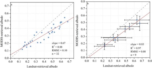
The accuracy of the MODIS albedo presented here is similar to that in previous work. Dumont et al. (2012) quantified that the mean difference between AWS measurements and the MOD10A1 product was 0.18 or approximately 27.5% relative error at Saint Sorlin Glacier in the Western Alps. Gunnarsson et al. (2021) reported the RMSE between the field measurements and MODIS albedo was 0.072, with R² of 0.9 for glaciers in Iceland. Wang et al. (2014) reported that the RMSE values for Palongzangbu glacier No. 4, Dongkemadi glacier, and Laohugou glaciers were 0.112, 0.068, and 0.064, respectively; and the R² values were 0.64, 0.69, and 0.72, respectively, based on a comparison between the MOD10A1 product and Landsat Thematic Mapper (TM)-retrieved albedo values calibrated by field measurements.

This underestimation may be attributed to the temporal aggregation of the MODIS albedo data, which introduced a dampening effect on the MODIS data compared with the Landsat-retrieved albedo. Tiny instantaneous snowfall events occurring before Landsat overpasses were not captured in the MODIS data due to the 11-day temporal aggregation. At the glacier-wide scale, the higher correlation coefficient, closer to 1:1 slope, and relatively lower RMSE indicated that the glacier-wide surface albedo was well captured by the gap-filling MODIS albedo.

4.2. Spatial distributions of Landsat-derived surface albedo during the ablation period

Figure 4 presents the spatial distribution of surface albedo values with significant differences during the ablation period of 2015. The images from May 28, August 16, and September 1 showed high values; more than 73% of the glacier surface had an albedo higher than 0.50 (typical value for snow albedo). The mean glacier-wide albedo values were 0.67, 0.63, and 0.61, respectively. A comparable spatial distribution of the surface albedo was found for these three images, with distinct differences of albedo value between the eastern and western parts of the same altitude bands. When the glacier was divided into five subregions as shown in Figure 5a, the differences between the mean albedo values of the same altitude band in different subregions was large, ranging from 0.24 to 0.49 (Figure 6). In every subregion, the signal of the increase in mean albedo with elevation was detected, namely usually so called the elevation effect on glacier albedo. For the #1 subregion, the main part of the Muz Taw Glacier, the maximum albedo was observed. The elevation effect on glacier albedo was remarkable below 3400 m a.s.l. (significant at 95% confidence level); the albedo elevation gradients were 0.031/100 m, 0.033/100 m, and 0.026/100 m, respectively on May 28, August 16, and September 1. Between 3400 m a.s.l. and 3600 m a.s.l., a slightly reduction in mean albedo from 0.80 to approximately 0.65 was seen. Above 3600 m a.s.l., the uptick was dominant, with significant fluctuations. For the other four subregions, the general upward trend in surface albedo with altitude was undisputed, especially above 3500 m a.s.l (significant at 90% confidence level except for #5 subregion). The linear albedo gradient varied over a wide range, between ∼0.012/100 m and ∼0.079/100 m.

Figure 4. Spatial distribution of Landsat-derived albedo at Muz Taw Glacier on selected dates of the ablation period in 2015.

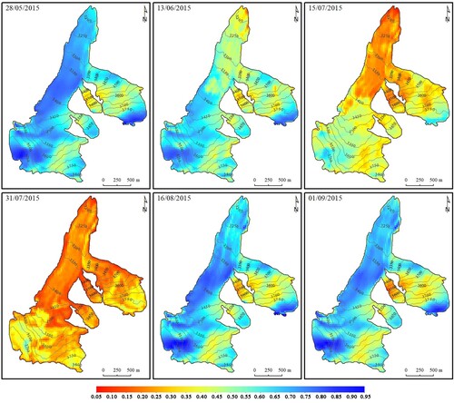
Figure 5. (a) The subregional divisions on Muz Taw Glacier and (b), (c), photographs taken on August 15, 2018, illustrating the variability of summer surface cover in different subregions on the same day. (b) The transition from clean ice in the #1 subregion to brownish-red ice in the #2 and #3 subregions. (c) Dark ice in the #4 subregion.

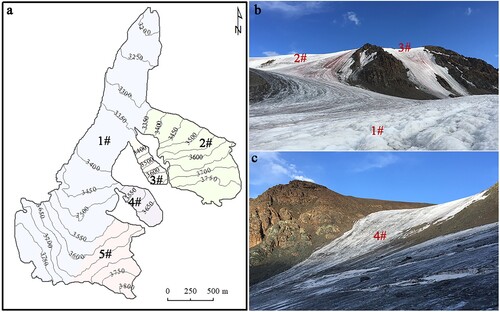
Figure 6. Mean albedo as a function of altitude in the five subregions shown in Figure 5a on selected dates. The light shadow envelopes around the mean represent the standard deviation of the average albedo.

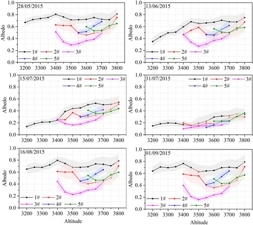
On 13 June, the mean glacier-wide albedo decreased to 0.57; approximately 69% of pixels had an albedo value greater than 0.50 (typical value for snow albedo), and 65% of these pixels were distributed in subregion #1. The east–west differences in surface albedo for the same altitude band were well maintained; the differences in mean albedo for the same altitude band of different subregions narrowed to between 0.12 and 0.38. Meanwhile, all subregions displayed a significant increase in surface albedo with altitude. Below 3450 m a.s.l of the #1 subregion, the increase in surface albedo was steady and rapid (significant at the 99% confidence level), with an albedo elevation gradient of 0.062/100 m. Above 3450 m a.s.l., the mean albedo of each altitude band in the #1 subregion was higher than that in other subregions, and little variation was observed, with mean albedo ranging from 0.65 to 0.75. For other subregions, the elevation effect in mean albedo remained pronounced above 3500 m a.s.l. (significant at the 90% confidence level except for #5 subregion), with average albedo elevation gradients of ∼0.011/100 m to ∼0.055/100 m.

On July 15, the mean glacier-wide albedo declined to 0.36, and 15.7% of pixels featured an albedo higher than 0.50 (typical value for snow albedo). East–west differences in surface albedo spatial distributions were visually attenuated, while this signal can still be captured by comparing the mean albedo of the same altitude zone in different subregions. The range of differences in mean albedo was further narrowed to 0–0.29 over all elevation bands. The trend of increasing albedo with altitude was more visually prominent than that on June 13 for the five subregions, which was in sharp contrast to the spatial pattern of surface albedo on May 28, August 16, or September 1. For the #1 subregion, the average albedo–elevation relationship showed two inflection points, at approximately 3400 m a.s.l. and 3600 m a.s.l. Below 3400 m a.s.l., the albedo elevation gradient was ∼0.024/100 m, and increased to ∼0.035/100 m at 3400–3600 m a.s.l (both significant at the 99% confidence level). Finally, the mean albedo stabilized at 0.50–0.54 above 3600 m a.s.l. The spatial pattern of surface albedo for the other four subregions was characterized by lower values and obvious increases with altitude (significant at the 95% confidence level except for the #5 subregion), and the albedo elevation gradients were concentrated in the range of 0.024/100 m to 0.043/100 m.

Finally, the mean glacier-wide albedo decreased to the minimum of 0.23 on July 31. Albedo values were almost all less than 0.50; 76.5% of the area had an albedo lower than 0.30 (typical value for ice albedo). The terminal part of the tongue and the western margin featured albedo values even lower than 0.20 (typical value for debris-rich ice albedo). Numerically, the two distinct spatial features of surface albedo exhibited earlier still existed, although their intensity was greatly weakened. The difference between the mean albedo of the same altitude band in different subregions was eventually limited to the range of 0.06–0.15. In the #1 subregion, the mean albedo remained stable in the range of 0.15–0.20 for elevations below 3450 m a.s.l. A sharp increase in surface albedo of 0.15 occurred in the middle of the glacier (approximately 3450–3600 m a.s.l.), with an albedo elevation gradient of ∼0.045/100 m. A slight increase in albedo followed above 3600 m a.s.l., with an albedo elevation gradient of ∼0.012/100 m. In the other subregions, a moderate increase in surface albedo was exhibited (significant at the 95% confidence level), and the albedo gradient ranged from 0.016/100 m to 0.037/100 m for the entire elevation range.

During the 2019 ablation period, the spatial distribution of surface albedo was similar to that in 2015 (Figure S2). On July 2 and July 18, although the missing data due to the scan-line corrector failure in the ETM+ data affected the investigation of surface albedo spatial distribution to some extent, the general increase with elevation and the east–west differences at the same elevation were still evident. On August 11 and August 27, the surface albedo elevation effect was dominant, especially in the #1 subregion. Compared with the #2 and #4 subregions, the east–west differences in surface albedo at the same altitude was more distinct in the #1, #3, and #5 subregions.

The spatial pattern of the albedo increase with altitude mainly reflected the glacier surface change from ice to snow cover. Over the melting glacier surface, the accumulation area is generally covered by snow, in contrast to the ablation area where ice is exposed and sometimes covered by debris. Therefore, as expected, the ablation area is characterized by lower albedo values than the accumulation area, exhibiting the surface albedo elevation effect. As a consequence, the position of the snow line can be identified in the albedo distribution map. Near the snow line, an albedo increase occurs over a short distance, the standard deviation of the distribution within an altitude band is rather large, and the albedo elevation gradient presents an inflection point (Yue et al. 2021). On May 28, August 16, and September 1, the majority of the glacier was covered by snow. The snow line was situated well below the snout of the glacier at an elevation of approximately 3150 m. On June 13, although the albedo sharply increased with altitude up to 3450 m and had a gentler increase with altitude above 3450 m, the albedo map revealed a blurry division between the ice and snow albedos; thus, no distinct position of the snow line was determined. At that time, the glacier surface below 3450 m was likely characterized by the snow–ice transition; above 3450 m, the glacier surface was dominated by snow cover. On July 15, the snow line was clear at an elevation of approximately 3400 m. Subsequently, the snow line retreated and reached an elevation of approximately 3450 m on July 31. In addition, over the bare-ice area or snow-cover area, the slight increase in albedo with altitude could be attributed to increased concentrations of light-absorbing impurities (LAIs). Zhang et al. (2020) reported an obvious reduction in LAI abundance with altitude on the Muz Taw Glacier during the ablation period.

The east–west differences in surface albedo for the same altitude band are probably related to the heterogeneity of LAI concentrations and the local terrain factors, such as slope, aspect and terrain inter-shielding. Field observations found that the glacier surface for the #2 and #3 subregions was mostly covered by brownish-red impurities (Figure 5b). This phenomenon is also observed on glaciers and snowfields worldwide, such as in Alaska (Ganey et al. 2017), Greenland (Ryan et al. 2018), and the Arctic (Lutz et al. 2016). The red snow is caused by blooms of snow algae that have carotenoid pigments in their cells, which reduce the surface albedo by absorbing the 400–600-nm shortwave radiation (Takeuchi et al. 2006, 2009). Similarly, the dark glacier surface contaminated with some dust and debris was also observed in the #4 subregion (Figure 5c). Research has shown that surface dust and debris significantly reduce glacier albedo, especially in the visible region (300–700 nm), where reflection by the glacier is strongest (e.g. Mauro et al. 2015; Baccolo et al. 2020; Yue et al. 2020). Thus, we deduced that the lower albedo on the eastern Muz Taw Glacier may result from the light-absorbing impurities, such as snow algae, black carbon, and mineral dust. The aspect of the eastern Muz Taw Glacier is northwest, which has longer exposure to solar radiation than the north-facing #1 subregion. As a consequence, more solar radiation accelerates the metamorphism and ablation of snow, causing lower surface albedo.

4.3. Temporal trends of MODIS-derived ablation-period albedo

The mean ablation-period albedo for the Muz Taw Glacier was 0.41 between 2000 and 2021, and varied from 0.35 in 2018 to 0.46 in 2002 (Figure 7a). A decline in annual ablation-period albedo was found throughout the studied period, and the linear regression indicated that the overall decreasing rate was approximately 0.019 (10 yr)⁻¹ implying the ablation-period albedo for Muz Taw Glacier decreased by 0.042 during the past 22 years (Table 4). In particular for May, a significant decrease of glacier-wide albedo was observed, of −0.033 (10 yr)⁻¹ (Table 4).

Figure 7. The (a) interannual and (b) seasonal variations in surface albedo for Muz Taw Glacier. (a) The boxes indicate the interquartile range of daily mean albedo. The whiskers represent the range of one standard deviation from the annual mean albedo. The median, mean, and maximum/minimum for individual years are shown by the short horizontal line, dot, and triangles, respectively. (b) The orange vertical lines indicate the dates of the albedo minima.

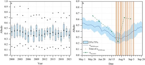
Table 4. Summary of mean (α), standard deviation (SD), temporal trend (Δα) and its significant level (P) of surface albedo at Muz Taw Glacier at monthly and entire ablation period timescales, 2000–2021, based on the average glacier-wide Moderate Resolution Imaging Spectroradiometer (MODIS) albedo.

	α	SD	Δα	P
${\alpha }_{ablation-period}$	0.41	0.04	–0.0019	0.135
${\alpha }_{May}$	0.51	0.06	–0.0033	0.097
${\alpha }_{June}$	0.45	0.06	–0.0012	0.564
${\alpha }_{July}$	0.34	0.07	–0.0008	0.734
${\alpha }_{August}$	0.31	0.05	–0.0019	0.263
${\alpha }_{September}$	0.43	0.08	–0.0014	0.635
${\alpha }_{ablation-period}^{min}$	0.15	0.03	–0.0030	0.005

The ablation period is from May through September. Ablation-period minimum albedo (${\alpha }_{ablation-period}^{min}$) and its variability is also shown.

Although the interannual decrease in the mean ablation-period albedo for Muz Taw Glacier is consistent with that of other adjacent glaciers, such as Urumqi Glacier No. 1, Glacier No. 354, and Laohugou glacier No. 12 (Zhang et al. 2021; Yue et al. 2022), the mean glacier-wide albedo value of Muz Taw Glacier was the lowest among them. The lower albedo is likely to be related to the concentration of light-absorbing impurities on the glacier surface and the snowfall in summer. Light-absorbing impurities, especially black carbon, substantially reduce the glacier albedo. Zhang et al. (2020) reported that average black carbon concentrations in the surface snow of the Muz Taw Glacier were 1788 ± 1741 ng g⁻¹, which were higher than those observed in Urumqi Glacier No. 1 (Ming et al. 2016) and Laohugou glacier No. 12 (Li et al. 2019). In addition, approximately 50% of the precipitation on Muz Taw Glacier occurs between May and September, while this percentage is usually much more 50% for other glaciers in Central Asia, such as approximately 88% for Urumqi Glacier No. 1 (Yang, Kang, and Felix 1992; Yue et al. 2017) and approximately 75% for Glacier No. 354 (Kronenberg et al. 2016). The lower precipitation between May and September, combined with the lower elevation, may result on less snowfall in summer at Muz Taw Glacier.

To characterize the overall variation of glacier-wide albedo though the ablation period, the mean seasonal evolution of glacier-wide albedo for the study period was obtained by averaging the daily MODIS values. On Muz Taw Glacier, MODIS data and Landsat data exhibit pronounced surface albedo seasonality (Figure 7b). The albedo generally declines from a maximum above 0.50 in May to a minimum below 0.30 in the last two weeks of July and first week of August, then gradually increases from August through to September. The variations of glacier-wide albedo during the ablation season are similar to those found in Iceland (Gunnarsson et al. 2021), the Rocky Mountains (Marshall and Miller 2020), the Alps (Dowson, Sirguey, and Cullen 2020), and the Himalayas (Brun et al. 2015). This cyclicality captures a series of surface process signals, and indicates that snow cover decreases at the beginning of ablation period until reaching its lowest extent, and finally increases again with the first snowfall.

For the minimum albedo, a large range was obtained, varying from 0.07 in 2021 to 0.22 in 2003 (Figure 7a). For 16 out of 22 years (73%) the minimum albedo was observed in August (Figure 7b). However, the minimum albedo can occur as early as the last week of July and as late as the first week of September. A significant negative temporal trend for the minimum albedo exists for 2000–2021, with a rate of approximately −0.03(10 yr)⁻¹ (Table 4). The minimum albedo provides insight into the relative share of exposed ice and snow-covered areas, which is also quantified by the accumulation–area ratio (AAR) or the equilibrium-line altitude (ELA) (Davaze et al. 2018). The remarkable decrease in the minimum glacier-wide albedo implied the decline of AAR, the rise of ELA, as well as more intense ablation over the past 22 years. Despite a large interannual variability for the timing of the minimum glacier-wide albedo over the period 2000–2021, no clear temporal trend during this period was found.

4.4. Mass-balance reconstruction using the albedo method, 2000–2015

Studying the variation in glacier-wide albedo during the ablation period can provide insight into the glacier mass balance (e.g. Brun et al. 2015; Sirguey et al. 2016; Davaze et al. 2018; Zhang et al. 2018). Hence, we assessed the relationship between the MODIS-derived mean albedo for the ablation season and the observed annual mass balances on Muz Taw Glacier (Figure 8a). Mean ablation-season glacier-wide albedo values correlate well with the annual mass balances, which is supported by a determination coefficient (R²) of 0.82 (n = 5; significant at the 95% confidence level with a Student’s t test). This suggested that the changes in ablation-season albedo can explain 82% of the annual mass-balance variability. Based on this significant correlational relationship between the two variables, the annual mass balance for years with available MODIS data was estimated using the so-called albedo method, and 16 years (2000–2015) of annual mass balance data for Muz Taw Glacier have been reconstructed. Leave-one-out cross validation illustrated that the uncertainty associated with the reconstructed values was 0.32 m w.e.

Figure 8. (a) Annual mass balance as a function of mean albedo for Muz Taw Glacier. The error bar for mean albedo is calculated as the accuracy of the Moderate Resolution Imaging Spectroradiometer (MODIS) albedo [root mean square error (RMSE) = 0.10] divided by the root mean square of the number of pixels in the average. The error bar for mass balance is the mean uncertainty of the geodetic mass balance, approximately ±0.18 m w.e. at Muz Taw Glacier. The red line illustrates the best fit line, along with the mean error prediction interval (red dashed line). (b) Annual mass balance and cumulative mass balance for the glacier. The reconstructed values are shown in gray, and the measured values are shown in blue.

The observed and reconstructed mass balances were averaged over their corresponding periods of record to allow comparison with the glacier-wide geodetic mass balance reported in Bai et al. (2022) for the period 2000–2016. Although a systematic bias may exist between the mass balance values obtained by different methods, this comparison allows us to examine the order of magnitude of our results. The calculated 2000–2016 cumulative mass balance was very close to the values obtained by the geodetic mass balance, although the former was slightly more negative than the latter (−13.9 ± 0.32 m w.e. vs −13.6 ± 0.46 m w.e.).

The difference probably results from the underestimation of MODIS albedo, glacier melting associated with other energy sources (e.g. turbulent fluxes), and the internal and basal components of the mass balance. First, the contribution of the underestimation of MODIS albedo to mass balance can be evaluated using incident shortwave radiation measured by the AWS at an elevation of 2900 m a.s.l. and approximately 6.5 km from the glacier. The years 2016 and 2018 were selected, with complete observed data during the ablation period. It was assumed that the quantity of net shortwave radiation resulting from the underestimation of MODIS albedo was all used to the glacier-surface melting. The calculated relative melt indicated that the 18% underestimation of albedo contributed approximately 11.5% and 9.0% to the glacier mass balance in 2016 and 2018, respectively. Second, because surface albedo only reflects the contribution of the shortwave radiative energy to glacier melting, it does not capture glacier melting associated with other energy sources. As a result, in theory, lower mass loss is calculated by the albedo method. Because the AWS data sets lack the surface-energy balance terms (i.e. net long-wave radiation, sensible and latent heat fluxes) required to compute the entire energy budget, calculating surface absolute melt was not possible. Third, geodetic surveys provide an estimate of the total mass change of a glacier, including surface, internal, and basal components of the mass balance, whereas the results inferred from the albedo method refer to the surface mass balance and do not account for the internal and basal components. Thus, the discrepancy between the mass balance obtained by the geodetic method and the albedo method was expected.

Figure 8b presents the annual mass-balance values and the corresponding cumulative mass balance for Muz Taw Glacier. A significant and continued mass loss was shown between 2000 and 2020. The maximum mass loss occurred in 2006, with a mass balance of approximately −1.35 ± 0.32 m w.e.; significant mass losses also occurred in 2008, 2010, 2011, 2017, and 2018, with an annual mass balance of more than −1.00 m w.e. Relatively less mass loss appeared in 2002 and 2019, with annual mass balances of less than −0.40 m w.e. By combining the observed and MODIS-derived values for 2000–2020, a cumulative mass balance of −17.3 ± 0.32 m w.e. was obtained, with an average mass balance of −0.82 ± 0.32 m w.e. yr⁻¹. Over the first 15 years of the twenty-first century, the 5-year mean mass balance showed accelerating mass loss, with mass balances of −0.53 ± 0.32 m w.e. per year for 2000–2004, −0.92 ± 0.32 m w.e. per year for 2005–2009, and −1.0 ± 0.32 m w.e. per year for 2010–2014. Since 2015, mass balance loss has slowed to -−0.89 ± 0.32 m w.e. per year.

In the first 20 years of the twenty-first century, the mean annual mass balance for Muz Taw Glacier was comparable to the average of global reference glaciers (−0.82 m w.e. yr⁻¹ vs −0.85 m w.e. yr⁻¹) (WGMS 2021). Chang et al. (2022) reported the mass loss was 14.55 ± 1.32 m w.e. (or −0.74 ± 0.07 m w.e. yr⁻¹) over the period 2000–2020 in the Altai Mountains based on a comparison of DEMs. Muz Taw Glacier experienced slightly more mass loss than adjacent Altai glaciers. Compared with adjacent glaciers, Muz Taw glacier also experienced the most intense ablation. For example, from 2000 to 2019, the cumulative mass loss for Muz Taw Glacier was twice as large as that of Tuyuksu glacier as well as 40% and 13% more than that of the western and eastern Urumqi glacier No.1, respectively. Nevertheless, among the three compared glaciers, Muz Taw Glacier showed a moderate year-to-year variability (standard deviation σ = 0.34 m w.e. for Muz Taw Glacier, 0.30 m w.e. for Urumqi glacier No.1 and 0.52 m w.e. for Tuyuksu glacier).

4.5. Summer snowfall, surface albedo and mass balance

Intermittent summer snowfall events not only directly increase the glacier accumulation but also temporarily refresh the glacier surface, reducing the number of ice exposure days on the glacier surface and, in turn, slowing the glacier melting. A detailed illustration of summer snowfalls during the ablation period is shown in Figure 9. Here, snowfalls were identified by the air-temperature threshold of 2°C, which was recommended by Zhang et al. (2017) based on the glacier mass balance model in the Altai Mountains. Specifically, precipitation is assumed to fall as snow at or below the threshold temperature, while it is assumed to be rain above the threshold temperature. A mixture of snow and rain probably occurs within a transition zone ranging from 1 K above to 1 K below the threshold temperature. To identify precipitation events more clearly, the raw precipitation data recorded by the T-200B is shown in Figure 9a, i.e. not calculated as the hourly specific precipitation quantity.

Figure 9. Example of summer snowfalls recorded at the Muz Taw Glacier automatic weather station site from July 15 to August 23, 2019. (a) The raw precipitation data recorded by the T-200B precipitation gauge, i.e. not calculated as hourly precipitation quantity. (b) Air temperature; the dashed lines represent the air temperature thresholds of 2°C for snow, and the blue shaded areas indicates the temperature range of the mixture of snow and rain. (c) Mean daily albedo. The grey shaded areas indicate the precipitation events.

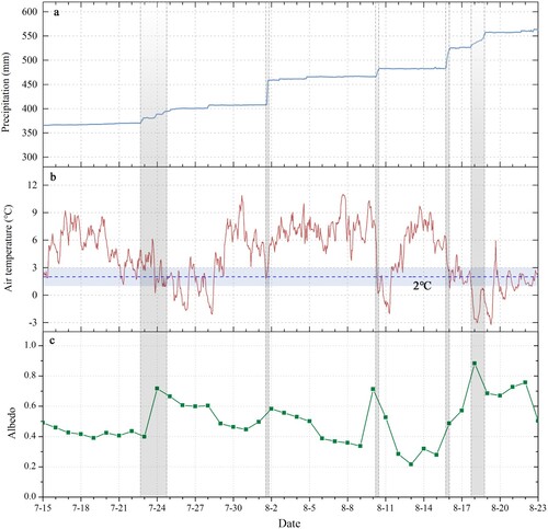
During a 40-day period from July 15 to August 23, 2019, there were five distinct snowfalls at the Muz Taw Glacier AWS site. The first occurred intermittently between the night of July 22 and the early morning of July 25, resulting in the albedo rising from 0.4 on July 23 to 0.7 on July 24. The air temperature was below 3°C for most of the next four days, and the surface albedo remained above 0.6. As the air temperature rose rapidly from the afternoon of July 28, surface albedo declined rapidly to approximately 0.45 on July 31. The second snowfall was concentrated in the afternoon to night of August 1, causing surface albedo to increase to 0.6 in the next day. After that, the air temperature stayed above 6°C, and surface albedo continued to decrease, returning to 0.4 again after approximately 4 days. As the air temperature rose further, the surface albedo eventually dropped to 0.35 on August 9. The third snowfall occurred in the morning of August 10, and surface albedo rose to 0.7 that day. Subsequently, driven by a rapid air-temperature increase, the surface albedo decreased rapidly and reached the lowest value of approximately 0.2 within three days. Between the afternoon and evening of August 15, and throughout the day of August 18, the fourth and fifth snowfalls occurred. The shorter interval between these two snowfalls, combined with a sustained drop in air temperature during this period, resulted in a sustained increase in surface albedo. On August 18, surface albedo increased to the maximum value over these 40 days, approximately 0.88. After that, air temperatures remained low, and surface albedo declined slightly.

If 0.4 is taken as the typical albedo value of the glacier surface over these 40 days, the snowfalls increased the mean albedo to 0.51. The calculated relative melt suggests that the increase in surface albedo of 0.11 reduces the average absorbed energy by approximately 24 W m⁻², equivalent to a 0.25 m w.e. decrease in melting over this 40-day period. The observed mean mass balance values, derived from five stake readings near the AWS (Figure 1b), were approximately −0.48 m w.e. between July 15 and August 23. Thus, the increase in surface albedo of 0.11 resulted in an approximately 52% reduction in glacier loss at the AWS site. Therefore, the indirect impact of snowfall on mass balance, through increased surface albedo and reduced melting, is remarkable.

5. Conclusions

Over the ablation period, the surface albedo derived from Landsat images showed that the spatial albedo pattern for Muz Taw Glacier was characterized by a general increase with elevation and significant east–west differences at the same elevation. The increase in albedo with altitude reflects the change of glacier surface from ice to snow cover. The east–west difference at the same altitude probably is related to the heterogeneous distribution of LAI concentrations and the local terrain (e.g. the aspect).

During the past 22 years (2000–2021), the gap-filling MODIS albedo indicated the mean ablation-period albedo for Muz Taw Glacier was 0.41, with a nonsignificant negative trend. A significant decrease of surface albedo was detected in May, with a temporal trend of −0.03 per decade. From May to September, glacier-wide albedo exhibited a pronounced, V-shaped seasonal variability. The minimum albedo generally occurred in August. The significant decrease in annual minimum albedo from 2000 to 2021 suggested the undisputed rise of ELA and increasing intense ablation.

Annual mass balances are highly sensitive to variations in mean ablation-period albedo. The changes in ablation-period albedo can explain 82% of the annual mass-balance variability. Thus, we applied the albedo method to estimate the annual mass balance for Muz Taw Glacier over the period 2000–2015. By combining observed and MODIS-derived values, the cumulative mass balance for the glacier was determined as −17.3 ± 0.32 m w.e. during the period 2000–2020, with accelerated mass loss.

Summer snowfall not only directly increases the glacier accumulation but also increase the surface albedo, thus substantially reducing the glacier melting. The impact of summer snowfalls on glacier mass balance is particularly pronounced in July and August, temporarily brightening the low-albedo glacier ice, and reducing the number of snow-free days on the glacier surface. Based on field observations for the period July 15–August 23, 2019, summer snowfalls decrease glacier melting by up to 52% at the Muz Taw Glacier AWS site. However, this is a preliminary estimate; further research is needed to systematically quantify the impact of albedo feedback on glacier mass balance using the energy–mass balance model.

Acknowledgements

We are grateful to NASA for the MODIS data and USGS for the Landsat images data. We also thank staff and students of the Altai Observation and Research Station of Cryospheric Science and Sustainable Development of the Chinese Academy of Science for their valuable support of the field work.

Data availability

MODIS data is available from https://modis.gsfc.nasa.gov/data/dataprod/mod10.php. Landsat OLI data is downloaded through https://earthexplorer.usgs.gov.

Disclosure statement

No potential conflict of interest was reported by the authors.

Additional information

Funding

This work was supported by the National Natural Science Foundation of China [grant number 42001066]; the Open-end Foundation for National Cryosphere Desert Data Center [grant number 20D05]; the Foundation for Excellent Youth Scholars of NIEER, CAS [grant number FEYS2019003]; State Key Laboratory of Cryospheric Science [grant number SKLCS-ZZ-2022]; and the Third Comprehensive Scientific Expedition of Xinjiang Uyghur Autonomous Region [grant number 2022xjkk0802, 2022xjkk0701].

References

- Alexander, P., M. Tedesco, X. Fettweis, R. S. W. Van de Wal, C. J. P. P. Smeets, and M. R. Van den Broeke. 2014. “Assessing Spatio-Temporal Variability and Trends in Modelled and Measured Greenland Ice Sheet Albedo (2000–2013).” The Cryosphere 8: 2293–2312. https://doi.org/10.5194/tc-8-2293-2014.
- Baccolo, G., E. Lokas, P. Gaca, D. Massabò, R. Ambrosini, R. S. Azzoni, C. Clason, et al. 2020. “Cryoconite: an Efficient Accumulator of Radioactive Fallout in Glacial Environments.” The Cryosphere 14: 657–672. https://doi.org/10.5194/tc-14-657-2020.
- Bai, C., F. Wang, Y. Bi, L. Wang, C. X. Yue, S. Yang, and P. Wang. 2022. “Increased Mass Loss of Glaciers in the Sawir Mountains of Central Asia Between 1959 and 2021.” Remote Sensing 14: 5406. https://doi.org/10.3390/rs14215406.
- Bippus, Gabriele.. 2011. Characteristics of Summer Snow Areas on Glaciers Observed by Means of Landsat Data: Correction Techniques for Optical Satellite Data.” PhD diss., University of Innsbruck.
- Box, J. E., X. Fettweis, J. C. Stroeve, M. Tedesco, D. K. Hall, and K. Steffen. 2012. “Greenland Ice Sheet Albedo Feedback: Thermodynamics and Atmospheric Drivers.” The Cryosphere 6: 821–839. https://doi.org/10.5194/tc-6-821-2012.
- Brun, F., M. Dumont, E. Berthier, M. F. Azam, J. M. Shea, P. Sigruey, A. Rabatel, and A. Ramanathan. 2015. “Seasonal Changes in Surface Albedo of Himalayan Glaciers from MODIS Data and Links with the Annual Mass Balance.” The Cryosphere 9 (1): 341–355. https://doi.org/10.5194/tc-9-341-2015.
- Chang, J., N. Wang, Z. Li, and D. Yang. 2022. “Accelerated Shrinkage of Glaciers in the Altai Mountains from 2000 to 2020.” Frontiers in Earth Science 10: 919051. https://doi.org/10.3389/feart.2022.919051.
- Chen, Y., G. Fang, H. Hao, and X. Wang. 2022. “Water use Efficiency Data from 2000 to 2019 in Measuring Progress Towards SDGs in Central Asia.” Big Earth Data 6 (1): 90–102. https://doi.org/10.1080/20964471.2020.1851891.
- CMA-CCC (China Meteoritical Administration Climate Change Center). 2021. Blue Book on Climate Change in China. Beijing: Science Press.
- Davaze, L., A. Rabatel, Y. Arnaud, P. Sigruey, D. Six, A. Letreguilly, and M. Dumont. 2018. “Monitoring Glacier Albedo as a Proxy to Derive Summer and Annual Surface Mass Balances from Optical Remote-Sensing Data.” The Cryosphere 12: 271–286. https://doi.org/10.5194/tc-12-271-2018.
- Dowson, A. J., P. Sirguey, and N. J. Cullen. 2020. “Variability in Glacier Albedo and Links to Annual Mass Balance for the Gardens of Eden and Allah, Southern Alps, New Zealand.” The Cryosphere 14: 3425–3448. https://doi.org/10.5194/tc-14-3425-2020.
- Dumont, M., J. Gardelle, P. Sirguey, A. Guillot, D. Six, A. Rabatel, and Y. Arnaud. 2012. “Linking Glacier Annual Mass Balance and Glacier Albedo Retrieved from MODIS Data.” The Cryosphere 6: 1527–1539. https://doi.org/10.5194/tc-6-1527-2012.
- Ekstrand, S. 1996. “Landsat TM-Based Forest Damage Assessment: Correction for Topographic Effects.” Photogrammetic Engineering & Remote Sensing 62 (2): 151–162.
- Fugazza, D., A. Senese, R. S. Azzoni, M. Maugeri, and G. A. Diolaiuti. 2016. “Spatial Distribution of Surface Albedo at the Forni Glacier (Stelvio National Park, Central Italian Alps).” Cold Regions Science and Technology 125: 128–137. https://doi.org/10.1016/j.coldregions.2016.02.006.
- Ganey, G. Q., M. G. Loso, A. B. Burgess, and R. J. Dial. 2017. “The Role of Microbes in Snowmelt and Radiative Forcing on an Alaskan Icefield.” Nature Geoscience 10: 754–759. https://doi.org/10.1038/ngeo3027.
- Greuell, W., and M. De Ruyter de Wildt. 1999. “Anisotropic Reflection of Melting Glacier Ice: Measurements and Parameterizations in Landsat TM Band 2 and 4.” Remote Sensing of Environment 70 (3): 265–277.
- Greuell, W., C. H. Reijmer, and L. Oerlemans. 2002. “Narrowband-to-Broadband Albedo Conversion for Glacier Ice and Snow Based on Aircraft and Near-Surface Measurements.” Remote Sensing of Environment 82: 48–63.
- Gunnarsson, A., S. M. Gardarsson, F. Pálsson, T. Jóhannesson, and Ó. G. B. Sveinsson. 2021. “Annual and Inter-Annual Variability and Trends of Albedo of Icelandic Glaciers.” The Cryosphere 15: 547–570. https://doi.org/10.5194/tc-15-547-2021.
- Gurgiser, W., B. Marzeion, L. Nicholson, M. Ortner, and G. Kaser. 2013. “Modeling Energy and Mass Balance of Shallap Glacier, Peru.” The Cryosphere 7: 1787–1802. https://doi.org/10.5194/tc-7-1787-2013.
- Hall, D. K., and G. A. Riggs. 2021a. MODIS/Aqua Snow Cover Daily L3 Global 500m SIN Grid, Version 61. [2002-2021]. Boulder, Colorado: NASA National Snow and Ice Data Center Distributed Active Archive Center.
- Hall, D. K., and G. A. Riggs. 2021b. MODIS/Terra Snow Cover Daily L3 Global 500m SIN Grid, Version 61. [2000-2021]. Boulder, Colorado: NASA National Snow and Ice Data Center Distributed Active Archive Center.
- Hock, R., and B. Holmgren. 2005. “A Distributed Surface Energy-Balance Model for Complex Topography and its Application to Storglaciären, Sweden.” Journal of Glaciology 51 (172): 25–36.
- Huai, B., Z. Li, F. Wang, W. Wang, P. Wang, and K. Li. 2015. “Glacier Volume Estimation from Ice-Thickness Data, Applied to the Muz Taw Glacier, Sawir Mountains, China.” Environmental Earth Sciences 74 (3): 1861–1870. https://doi.org/10.1007/s12665-015-4435-2.
- Huss, M., and R. Hock. 2018. “Global-scale Hydrological Response to Future Glacier Mass Loss.” Nature Climate Change 8: 135–140. https://doi.org/10.1038/s41558-017-0049-x.
- Johnson, E., and S. Rupper. 2020. “An Examination of Physical Processes That Trigger the Albedo-Feedback on Glacier Surfaces and Implications for Regional Glacier Mass Balance Across High Mountain Asia.” Frontiers in Earth Science 8: 129. https://doi.org/10.3389/feart.2020.00129.
- Jonsell, U., R. Hock, and B. Holmgren. 2003. “Spatial and Temporal Variations in Albedo on Storglaciären, Sweden.” Journal of Glaciology 49 (164): 59–68.
- Kadota, T., and D. Gombo. 2007. “Recent Glacier Variations in Mongolia.” Annals of Glaciology 46: 185–188.
- Klein, A. G., and J. Stroeve. 2002. “Development and Validation of a Snow Albedo Algorithm for the MODIS Instrument.” Annals of Glaciology 34: 45–52.
- Klok, E. J., W. Greull, and J. Oerlemans. 2003. “Temporal and Spatial Variation of the Surface Albedo of Morteratschgletscher, Switzerland, as Derived from 12 Landsat Images.” Journal of Glaciology 49 (167): 491–502.
- Klok, E. J., and J. Oerlemans. 2004. “Modelled Climate Sensitivity of the Mass Balance of Morteratschgletscher and its Dependence on Albedo Parameterization.” International Journal of Climatology 24: 231–245.
- Kronenberg, M., M. Barandun, M. Hoelzle, M. Huss, D. Farinotti, E. Azisov, R. Usubaliev, A. Gafurov, D. Petrakov, and A. KääB. 2016. “Mass-balance Reconstruction for Glacier No. 354, Tien Shan, from 2003 to 2014.” Annals of Glaciology 57 (71): 92–102. https://doi.org/10.3189/2016AoG71A032.
- Li, Y., S. Kang, J. Chen, Z. Hu, K. Wang, R. Paudyal, J. Liu, X. Wang, X. Qin, and M. Sillanpää. 2019. “Black Carbon in a Glacier and Snow Cover on the North-Eastern Tibetan Plateau: Concentrations, Radiative Forcing and Potential Source from Local Topsoil.” Science of The Total Environment 686 (10): 1030–1038. https://doi.org/10.1016/j.scitotenv.2019.05.469.
- Lu, J., Y. Qiu, X. Wang, W. Liang, P. Xie, L. Shi, M. Menenti, and D. Zhang. 2020. “Constructing Dataset of Classified Drainage Areas Based on Surface Water-Supply Patterns in High Mountain Asia.” Big Earth Data 4 (3): 225–241. https://doi.org/10.1080/20964471.2020.1766180.
- Lutz, S., A. M. Anesio, R. Raiswell, A. Edwards, R. Newton, F. Gill, and L. G. Benning. 2016. “The Biogeography of red Snow Microbiomes and Their Role in Melting Arctic Glaciers.” Nature Communications 7: 11968. https://doi.org/10.1038/ncomms11968.
- Marshall, S. J., and K. Miller. 2020. “Seasonal and Interannual Variability of Melt-Season Albedo at Haig Glacier, Canadian Rocky Mountains.” The Cryosphere 14: 3249–3267. https://doi.org/10.5194/tc-14-3249-2020.
- Masek, J. G., E. F. Vermote, N. E. Saleous, R. Wolfe, F. G. Hall, K. F. Huemmrich, F. Gao, J. Kutler, and T. K. Lim. 2006. “A Landsat Surface Reflectance Dataset for North America, 1990–2000.” IEEE Geoscience and Remote Sensing Letters 3 (1): 68–72. https://doi.org/10.1109/LGRS.2005.857030.
- Mauro, B. D., F. Fava, L. Ferrero, R. Garzonio, G. Baccolo, B. Delmonte, and R. Colombo. 2015. “Mineral Dust Impact on Snow Radiative Properties in the European Alps Combining Ground, UAV, and Satellite Observations.” Journal of Geophysical Research: Atmospheres 120: 6080–6097. https://doi.org/10.1002/2015JD023287.
- Ming, J., C. Xiao, F. Wang, Z. Li, and Y. Li. 2016. “Grey Tienshan Urumqi Glacier No.1 and Light-Absorbing Impurities.” Environmental Science and Pollution Research 23 (10): 9549–9558. https://doi.org/10.1007/s11356-016-6182-7.
- Moustafa, S. E., A. K. Rennermalm, L. C. Smith, M. A. Miller, J. R. Mioduszewski, L. S. Koenig, M. G. Hom, and C. A. Shuman. 2015. “Multi-modal Albedo Distributions in the Ablation Area of the Southwestern Greenland Ice Sheet.” The Cryosphere 9: 905–923. https://doi.org/10.5194/tc-9-905-2015.
- Naegeli, K., and M. Huss. 2017. “Sensitivity of Mountain Glacier Mass Balance to Changes in Bare-ice Albedo.” Annals of Glaciology 58(75py2): 119–129. https://doi.org/10.1017/aog.2017.25.
- Naegeli, K., M. Huss, and M. Hoelzle. 2019. “Change Detection of Bare-ice Albedo in the Swiss Alps.” The Cryosphere 13: 397–412.
- NASA/METI/AIST/Japan Spacesystems, and U.S./Japan ASTER Science Team. 2018. “ASTER Global Digital Elevation Model V003.” NASA EOSDIS Land Processes DAAC. https://doi.org/10.5067/ASTER/ASTGTM.003.
- Oerlemans, J., R. H. Giesen, and M. R. Van Den Broeke. 2009. “Retreating Alpine Glaciers: Increased Melt Rates Due to Accumulation of Dust (Vadret da Morteratsch, Switzerland).” Journal of Glaciology 55 (192): 729–736.
- Panagiotopoulos, F., M. Shahgedanova, A. Hannachi, and D. B. Stephenson. 2005. “Observed Trends and Teleconnections of the Siberian High: A Recently Declining Center of Action.” Journal of Climate 18: 1411–1422.
- Paul, F., N. Barrand, S. Baumann, E. Berthier, T. Bolch, K. Casey, H. Frey, S. P. Joshi, V. Konovalov, R. Lebris, et al. 2013. “On the Accuracy of Glacier Outlines Derived from Remote-Sensing Data.” Annals of Glaciology 54 (63): 171–182. https://doi.org/10.3189/2013AoG63A296.
- Reijmer, C. H., R. Bintanja, and W. Greuell. 2001. “Surface Albedo Measurements Over Snow and Blue Ice in Thematic Mapper Bands 2 and 4 in Dronning Maud Land, Antarctica.” Journal of Geophysical Research: Atmospheres 106 (D9): 9661–9672.
- RGI. 2017. Randolph Glacier Inventory – A Dataset of Global Glacier Outlines: Version 6.0: Technical Report, Global Land Ice Measurements from Space. Colorado, AZ: Digital Media.
- Roe, G. H., M. B. Baker, and F. Herla. 2017. “Centennial Glacier Retreat as Categorical Evidence of Regional Climate Change.” Nature Geoscience 10: 95–99. https://doi.org/10.1038/ngeo2863.
- Ryan, J. C., A. Hubbard, M. Stibal, T. D. Irvine-Fynn, J. Cook, L. C. Smith, K. Cameron, and J. Box. 2018. “Dark Zone of the Greenland Ice Sheet Controlled by Distributed Biologically-Active Impurities.” Nature Communications 9: 1065. https://doi.org/10.1038/s41467-018-03353-2.
- Schaefer, M., D. Fonseca-Gallardo, D. Farías-Barahona, and G. Casassa. 2020. “Surface Energy Fluxes on Chilean Glaciers: Measurements and Models.” The Cryosphere 14: 2545–2565. https://doi.org/10.5194/tc-14-2545-2020.
- Shahgedanova, M., G. Nosenko, T. Khromova, and A. Muraveyev. 2010. “Glacier Shrinkage and Climatic Change in the Russian Altai from the mid-20th Century: An Assessment Using Remote Sensing and PRECIS Regional Climate Model.” Journal of Geophysical Research 115: D16107. https://doi.org/10.1029/2009JD012976.
- Shuai, Y., L. Tuerhanjian, C. Shao, F. Gao, Y. Zhou, D. Xie, T. Liu, and N. Chu. 2020. “Re-understanding of Land Surface Albedo and Related Terms in Satellite-Based Retrievals.” Big Earth Data 4 (1): 45–67. https://doi.org/10.1080/20964471.2020.1716561.
- Sirguey, P., H. Still, N. J. Cullen, M. Dumont, Y. Arnaud, and J. P. Conway. 2016. “Reconstructing the Mass Balance of Brewster Glacier, New Zealand, using MODIS-Derived Glacier-Wide Albedo.” The Cryosphere 10: 2465–2484. https://doi.org/10.5194/tc-10-2465-2016.
- Su, B., C. Xiao, D. Chen, Y. Huang, Y. Che, H. Zhao, M. Zou, R. Guo, X. Wang, X. Li, et al. 2022. “Glacier Change in China Over Past Decades: Spatiotemporal Patterns and Influencing Factors.” Earth-Science Reviews 226: 103926. https://doi.org/10.1016/j.earscirev.2022.103926.
- Surazakov, A. B., V. B. Aizen, E. M. Aizen, and S. A. Nikitin. 2007. “Glacier Changes in the Siberian Altai Mountains, Ob River Basin, (1952–2006) Estimated with High Resolution Imagery.” Environmental Research Letters 2 (4): 045017. https://doi.org/10.1088/1748-9326/2/4/045017.
- Takeuchi, N. 2009. “Temporal and Spatial Variations in Spectral Reflectance and Characteristics of Surface Dust on Gulkana Glacier, Alaska Range.” Journal of Glaciology 55 (192): 701–709.
- Takeuchi, N., R. Dial, S. Kohshima, T. Segawa, and J. Uetake. 2006. “Spatial Distribution and Abundance of red Snow Algae on the Harding Icefield, Alaska Derived from a Satellite Image.” Geophysical Research Letters 33: L21502. https://doi.org/10.1029/2006GL027819.
- Tedesco, M., S. Doherty, X. Fettweis, P. Alexander, J. Jeyavinoth, and J. Stroeve. 2016. “The Darkening of the Greenland ice Sheet: Trends, Drivers, and Projections (1981–2100).” The Cryosphere 10: 477–496. https://doi.org/10.5194/tc-10-477-2016.
- Vermote, E., C. Justice, M. Claverie, and B. Franch. 2016. “Preliminary Analysis of the Performance of the Landsat 8/OLI Land Surface Reflectance Product.” Remote Sensing of Environment 185: 46–56. https://doi.org/10.1016/j.rse.2016.04.008.
- Wang, Z., A. M. Erb, C. B. Schaaf, Q. Sun, Y. Liu, Y. Yang, Y. Shuai, K. A. Casey, and M. O. Román. 2016. “Early Spring Post-Fire Snow Albedo Dynamics in High Latitude Boreal Forests Using Landsat-8 OLI Data.” Remote Sensing of Environment 185: 71–83. https://doi.org/10.1016/j.rse.2016.02.059.
- Wang, F., C. Xu, Z. Li, M. N. Anjum, and L. Wang. 2018. “Applicability of an Ultra-Long-Range Terrestrial Laser Scanner to Monitor the Mass Balance of Muz Taw Glacier, Sawir Mountains, China.” Sciences in Cold and Arid Regions 10 (1): 47–54.
- Wang, J., B. Ye, Y. Cui, X. He, and G. Yang. 2014. “Spatial and Temporal Variations of Albedo on Nine Glaciers in Western China from 2000 to 2011.” Hydrological Processes 28: 3454–3465. https://doi.org/10.1002/hyp.9883.
- Wang, Y., J. Zhao, Z. Li, and M. Zhang. 2019. “Glacier Changes in the Sawuer Mountain during 1977–2017 and their Response to Climate Change.” [in Chinese.] Journal of Natural Resources 34 (4): 802–814.
- Wei, J., S. Liu, J. Xu, W. Guo, W. Bao, D. Shangguan, and Z. Jiang. 2015. “Mass Loss from Glaciers in the Chinese Altai Mountains Between 1959 and 2008 Revealed Based on Historical Maps, SRTM, and ASTER Images.” Journal of Mountain Science 12 (2): 330–343. https://doi.org/10.1007/s11629-014-3175-1.
- WGMS (World Glacier Monitoring Service). 2021. Global Glacier Change Bulletin No. 4 (2018–2019). Zurich, Switzerland. Publication Based on Database Version. https://doi.org/10.5904/wgms-fog-2021-05.
- Xu, C., Z. Li, F. Wang, and J. Mu. 2021. “Spatio-temporal Changes of Mass Balance in the Ablation Area of the Muz Taw Glacier, Sawir Mountains, from Multi-Temporal Terrestrial Geodetic Surveys.” Remote Sensing 13: 1465. https://doi.org/10.3390/rs13081465.
- Yang, D., E. Kang, and B. Felix. 1992. “Characteristics of Precipitation in the Source Area of the Urumqi River Basin.” [in Chinese.] Journal of Glaciology and Geocryology 14: 258–266.
- Yang, M., X. Wang, G. Pang, G. Wan, and Z. Liu. 2019. “The Tibetan Plateau Cryosphere: Observations and Model Simulations for Current Status and Recent Changes.” Earth-Science Reviews 190: 353–369.
- Yue, X., Z. Li, H. Li, F. Wang, and S. Jin. 2022. “Multi-Temporal Variations in Surface Albedo on Urumqi Glacier No.1 in Tien Shan, Under Arid and Semi-Arid Environment.” Remote Sensing 14: 808. https://doi.org/10.3390/rs14040808.
- Yue, X., Z. Li, J. Zhao, J. Fan, N. Takeuchi, and L. Wang. 2020. “Variation in Albedo and its Relationship with Surface Dust at Urumqi Glacier No. 1 in Tien Shan, China.” Frontiers in Earth Science 8: 110. https://doi.org/10.3389/feart.2020.00110.
- Yue, X., Z. Li, J. Zhao, H. Li, P. Wang, and L. Wang. 2021. “Changes in the End-of-Summer Snow Line Altitude of Summer-Accumulation-Type Glaciers in the Eastern Tien Shan Mountains from 1994 to 2016.” Remote Sensing 13: 1080. https://doi.org/10.3390/rs13061080.
- Yue, X., J. Zhao, Z. Li, M. Zhang, J. Fan, L. Wang, and P. Wang. 2017. “Spatial and Temporal Variations of the Surface Albedo and Other Factors Influencing Urumqi Glacier No. 1 in Tien Shan, China.” Journal of Glaciology 63 (24): 899–911. https://doi.org/10.1017/jog.2017.57.
- Zemp, M., M. Hoelzle, and W. Haeberli. 2009. “Six Decades of Glacier Mass-Balance Observations: A Review of the Worldwide Monitoring Network.” Annals of Glaciology 50 (50): 101–111.
- Zemp, M., M. Huss, E. Thibert, N. Echert, R. McNabb, J. Huber, M. Barandun, H. Machguth, S. U. Nussbaumer, I. Gärtner-Roer, et al. 2019. “Global Glacier Mass Changes and Their Contributions to Sea-Level Rise from 1961 to 2016.” Nature 568: 382–386. https://doi.org/10.1038/s41586-019-1071-0.
- Zhang, Y., H. Enomoto, T. Ohata, H. Kitabata, T. Kadota, and Y. Hirabayashi. 2017. “Glacier Mass Balance and its Potential Impacts in the Altai Mountains Over the Period 1990–2011.” Journal of Hydrology 553: 662–677.
- Zhang, Y., T. Gao, S. Kang, D. Shangguan, and X. Luo. 2021. “Albedo Reduction as an Important Driver for Glacier Melting in Tibetan Plateau and its Surrounding Areas.” Earth-Science Reviews 220: 103735. https://doi.org/10.1016/j.earscirev.2021.103735.
- Zhang, Y., T. Gao, S. Kang, M. Sprenger, S. Tao, W. Du, J. Yang, F. Wang, and W. Meng. 2020. “Effects of Black Carbon and Mineral Dust on Glacial Melting on the Muz Taw Glacier, Central Asia.” Science of the Total Environment 740: 140056. https://doi.org/10.1016/j.scitotenv.2020.140056.
- Zhang, Z., L. Jiang, L. Liu, Y. Sun, and H. Wang. 2018. “Annual Glacier-Wide Mass Balance (2000-2016) of the Interior Tibetan Plateau Reconstructed from MODIS Albedo Products.” Remote Sensing 10: 1031. https://doi.org/10.3390/rs10071031.
- Zheng, G., S. K. Allen, A. Bao, J. A. Ballesteros-Cánovas, M. Huss, G. Zhang, J. Li, Y. Yuan, L. Jiang, et al. 2021. “Increasing Risk of Glacial Lake Outburst Floods from Future Third Pole Deglaciation.” Nature Climate Change 11: 411–417. https://doi.org/10.1038/s41558-021-01028-3.