Precision silviculture: use of UAVs and comparison of deep learning models for the identification and segmentation of tree crowns in pine crops

ABSTRACT

The monitoring of trees is crucial for the management of large areas of forest cultivations, but this process may be costly. However, remotely sensed data offers a solution to automate this process. In this work, we used two neural network methods named You Only Look Once (YOLO) and Mask R-CNN to overcome the challenging tasks of counting, detecting, and segmenting high dimensional Red–Green–Blue (RGB) images taken from unmanned aerial vehicles (UAVs). We present a processing framework, which is suitable to generate accurate predictions for the aforementioned tasks using a reasonable amount of labeled data. We compared our method using forest stands of different ages and densities. For counting, YOLO overestimates 8.5% of the detected trees on average, whereas Mask R-CNN overestimates a 4.7% of the trees. For the detection task, YOLO obtains a precision of 0.72 and a recall of 0.68 on average, while Mask R-CNN obtains a precision of 0.82 and a recall of 0.80. In segmentation, YOLO overestimates a 13.5% of the predicted area on average, whereas Mask R-CNN overestimates a 9.2%. The proposed methods present a cost-effective solution for forest monitoring using RGB images and have been successfully used to monitor $\sim 146,500$ acres of pine cultivations.

KEYWORDS:

• Artificial intelligence
• tree identification
• forestry
• remote sensing

1. Introduction

Methods of forest cultivation require constant monitoring to determine the condition of the trees, estimate densities, mortality ratios, manage pruning, and replant species efficiently. However, traditional technologies for counting trees or disease detection that rely on manual sampling are difficult and time-consuming when covering large areas. Therefore, new technologies such as Unmanned aerial vehicles (UAVs) and automated algorithms have been required to deal with the challenges of forest monitoring.

A broad array of methods have been developed to monitor forest cultivations from airborne imagery. For instance Wulder, Niemann, and Goodenough (2000); Pouliot et al. (2002); Park et al. (2011); Santoro et al. (2013) used Local maxima filtering algorithm for tree detection and crown segmentation. Also, Graves et al. (2016) used support vector machines for image classification using an imbalanced dataset of tree crowns. However, in the latest couple of years, deep neural network approaches have underwent significant advances in remote sensing applications (Zhang, Zhang, and Du 2016; Ma et al. 2019). For instance, Paoletti et al. (2018) used convolutional neural networks (CNN; Fukushima 1980; Lecun et al. 1998) for hyperspectral image classification. Poblete-Echeverría et al. (2017) perform detection and segmentation of vine canopy from RGB images using artificial neural networks (ANN). Their results demonstrate that ANN perform better than random forests which are in turn better than the k-means algorithm. Fricker et al. (2019) apply CNN to recognize different species of pine trees using multispectral (RGB) and hyperspectral imagery. Ampatzidis and Partel (2019) used the state-of-the-art YOLOv3 (Redmon and Farhadi 2018) object detection model to count and detect citrus-trees to evaluate individual tree health using multispectral imagery (RGB and red, near-red, and blue). Zhao et al. (2018) segmented regions of pomegranate trees using two CNN methods: Mask R-CNN (He et al. 2017) and U-Net (Ronneberger, Fischer, and Brox 2015), using optical imaging. They conclude that Mask R-CNN performs better than U-Net in terms of segmentation. Lastly, Wang et al. (2019) used light detection and ranging (LiDAR) data for tree segmentation using the Faster R-CNN (Ren et al. 2015) algorithm. Similar methods have been applied to natural forests (Surovỳ, Almeida Ribeiro, and Panagiotidis 2018; Onishi and Ise 2021), coniferous forest (Fricker et al. 2019; Katoh and Gougeon 2012), agroforestry (Graves et al. 2016), urban trees (Hassaan et al. 2016; Hartling et al. 2019), and tree crops like chestnuts trees (Marques et al. 2019), citrus (Santoro et al. 2013; Ampatzidis and Partel 2019; Csillik et al. 2018) and eucalyptus (Wallace, Musk, and Lucieer 2014).

In this work, we are interested in the challenging tasks of counting, detecting, and segmenting pine (genus Pinus) trees from high-dimensional RGB images taken from UAVs. We used two aforementioned state-of-the-art deep learning models for monitoring Pinus cultivations. Specifically, we used the object detection method YOLO (Redmon et al. 2016) and the instance segmentation method Mask-RCNN (He et al. 2017) for the same tasks of counting, detecting, and segmenting trees. As discussed before, both algorithms have been demonstrate to be effective in similar tasks (Zhao et al. 2018; Ampatzidis and Partel 2019). We compare the methods using plantations of different ages and densities. Through our experimentation, we show that (i) both models generate small (lower than $10\text{\%}$) average relative errors, (ii) despite YOLO achieves lower precision than Mask R-CNN either for detection and segmentation, errors are mainly associated with the threshold used to associate labels and their ground truth. This threshold can be varied depending on how precise we want to locate the trees.

Ultimately, our work presents an effective solution for RGB images, that is cheaper than adding red-edge, near-red (Panteleris, Oikonomidis, and Argyros 2018), depth (RGB-D) (Lange et al. 2012) or the high-cost hyperspectral and LIDAR technologies used in previous works. Lastly, we present our processing framework, which has been successfully used to monitor $\sim 146,500$ acres of Pine crops to date, using reasonable labeling efforts.

The following sections are organized as follows: Section 2 shows our case of study, the processing framework, and details about the methods we adopted. Section 3 presents our results and we discuss some important results. In Section 4, we analyze our main findings. Finally, Section 5 presents the conclusion of our work.

2. Materials and methods

2.1. Data acquisition

We use four forest stands of pine cultivations belonging to the same Pinaceae (genus Pinus) family, located in Chile and Argentina. Specifically, a 91-acre 1-year-old Pinus taeda plantation located at lat –26.032${}^{\circ }$ lon $-{54.45}^{\circ }$, a 32-acre 5-year-old Pinus radiata plantation located at lat $-35.118$ lon $-72.038$, a 227-acre 8-year-old Pinus radiata plantation located at lat $-40.131$ lon $-73.122$, and a 336-acre 10-year-old Pinus radiata plantation located at lat $-{35.201}^{\circ }$ lon $-{72.182}^{\circ }$. A map of the selected areas is displayed in Figure 1. Images from each forest stand with the respective age of its trees are displayed in Figure 2. As can be seen, the distribution of the areas between the stands may vary, and we can observe that forest stands with older trees are denser.

Figure 1. Map of the selected areas for the study. Red points are the locations of the selected areas.

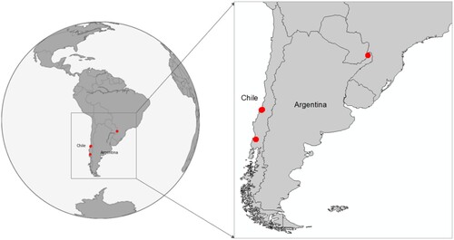
Figure 2. Images from the Pinus radiata's forest stands used in this work. Each stand has trees of the same age. It can be seen that the density of the plantation increases with the age of the trees. Therefore, some trees may overlap in older plantations.

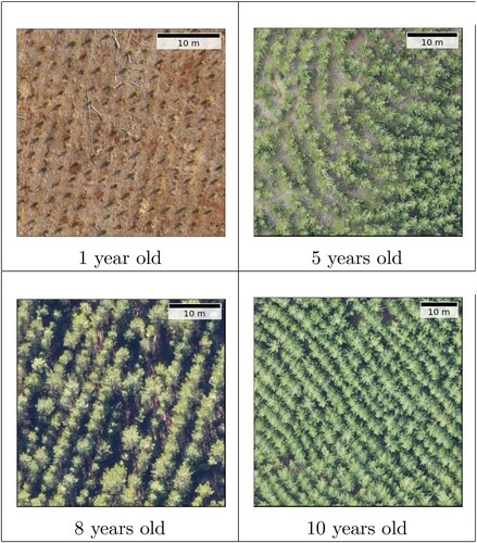
Image acquisition was made using a DJI-Phantom 3 drone UAV. A RGB camera with a blue (820–860 nm), green (550–570 nm) and red (663–673 nm) imaging sensors and a resolution of 12 megapixels was mounted under the UAV, and an orthomosaic image was created using the DroneDeploy software.¹ In Figure 3, we show one complete forest after being processed. Note that in this problem, the regions of interest are known in advance and they are demarcated with black lines. Therefore, we only use these regions of interest. Table 1 provides a summary of the forest stands used in this work.

Figure 3. Example forest stand of a 5-year-old Pinus radiata used in this work. The black lines indicate the borders of the regions of interest.

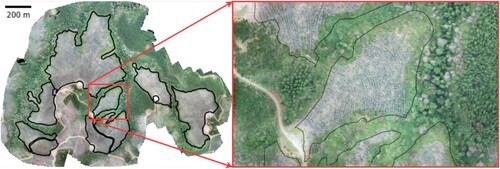
Table 1. Summary of the information for the forest stands used in this work.

Age (years)	Specie	Area (acres)	GSD (m)	Flying height (m)	Lat	Lon	Average crown diameter (m)
1	Pinus Taeda	91	0.047	210	26.032${}^{\circ }$	$-{54.45}^{\circ }$	1.36
5	Pinus Radiata	32	0.061	270	35.118	$-72.038$	2.62
8	Pinus Radiata	227	0.057	252	40.131	$-73.122$	3.14
10	Pinus Radiata	336	0.081	360	35.201${}^{\circ }$	$-{72.182}^{\circ }$	3.82

2.2. Pre-processing

For large forest stands, the amount of data is enough to train deep learning models. However, the use of these models is not straightforward because we need to define the input. Also, for the deep learning models used in this work, a manual labeling process is needed for training and evaluation. Therefore, a strategy to generate labels from the forest stands is needed.

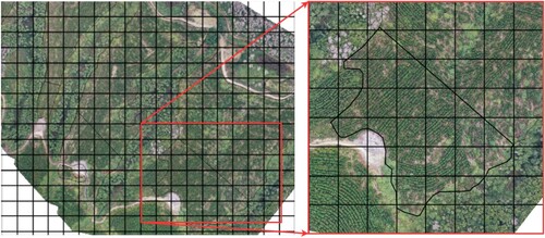
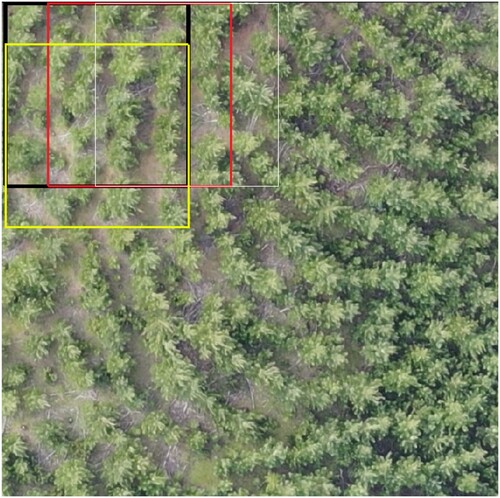
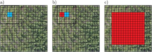
We use a strategy that can be described in two steps. In the first step, we create standard square grids of a fixed number of pixels. We chose a size of $768\times 768$ pixels, covering areas between 36 m${}^2$ and 62 m${}^2$ (as given by the GSDs shown in Table 1), which comprises an amount of trees that a human can easily label. However, the size of the grid elements may be changed if needed. As will be seen in Section 2.4, five of these grids are selected to create the training, testing, and evaluation sets. An example of this process is depicted in Figure 4.

Figure 4. The first step of our pre-process divides the forest stand in grid cells of size $768\times 768$ (represented by black squares). Later, some grid cells are used for labeling.

In the second step, we subdivide each element of the grid into smaller sub-images that will be used as inputs for the models. We can think of a simple division of $3\times 3$ sub-images of $256\times 256$ pixels each. This subdivision, however, creates limited labeled data per grid. The use of few labels can impact the performance of our model. Instead, we use an overlapped subdivision of each element of the grid. We use images of $256\times 256$ pixels and, starting from the top left, we move 64 pixels to the right to obtain a second image; we repeat this process eight times until reaching the boundary. Then, starting again from the top left, we move 64 pixels downwards, and we repeat the aforementioned process. We obtain in total 81 ($9\times 9$) sub-images for each element of the grid. Figure 5 shows part of this process. For evaluation, we made a special treat for the trees found at the edges (see Section 2.5 for details).

Figure 5. The second step of our pre-process subdivides the grid into smaller overlapped sub-images of size $256\times 256$ (represented by colored squares). We train our models using the sub-images and their respective labels.

Although we focus on Pinus plantations, our approach can be adapted and used to detect other species. This generality comes from the supervision of our model. This means that for different age forest stands, manual labeling is needed. However, we note that the number of labeled grids needed to train accurate models is less than 2% of the entire image field.

2.3. Methods

In this work, we exploit the power of state-of-the-art methods named YOLO (Redmon et al. 2016) and Mask-RCNN (He et al. 2017) to compare their performances in counting, detection, and segmentation tasks.

2.3.1. YOLO

Object detection refers to the task of allocating objects in an image and generate bounding boxes around objects of interest. Based on CNN You only look once (YOLO Redmon et al. (2016)) is one of the most popular neural network models for object detection. YOLO optimizes a single convolutional network architecture to simultaneously predict classes and bounding boxes for a given input. Without fully connected layers involved during training, the YOLO architecture offers an end-to-end training model with high accuracy and inference speed ($\ge 30$FPS).

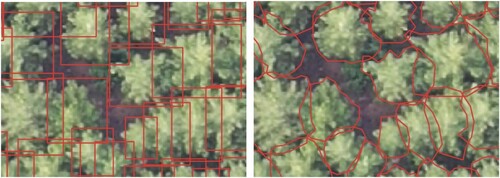
As in the standard supervised learning setting, a labeling process is needed for training. An example of the bounding boxes used as labels to train the YOLO model displayed in Figure 6 Left. Notice that labels are obtained by visual interpretation of the images. As can be seen, trees can be overlapped and this happen frequently in older plantations. One advantage of YOLO is that it is capable of dealing with these cases. Also, the CNN architecture allows feeding the network with different image sizes, bringing the possibility of increasing the size of an image to detect smaller objects without changing the model architecture.

Figure 6. Left: Labels needed to train the YOLO model. Right: Labels needed to train the Mask-RCNN model. As can be seen, Mask R-CNN labels are made by drawing polygons around the canopy trees, and YOLO labels are made drawing a simpler rectangle. This difference makes Mask R-CNN labels harder to obtain. Labels are obtained by drawing the shapes by visual inspection of the image using QGIS software functionalities (QGIS Development Team 2022).

Several improvements have been made to the original YOLO system. The last version developed by the original authors (YOLOv3 Redmon and Farhadi (2018)). Speeds of up to 45 FPS can be achieved with this method. For all our experiments, we used YOLOv3 implemented using PyTorch (Paszke et al. 2019), and the Darknet53 CNN architecture pretrained on COCO dataset as the model architecture. Experiments were performed using an NVIDIA Tesla P100 GPU in a Google Cloud Platform instance.

2.3.2. Mask R-CNN

Instance segmentation considers object detection plus semantic segmentation (i.e. pixel by pixel classification). Therefore, in this task we are interested in segment each of the three crowns individually. We use the instance segmentation model named Mask R-CNN (He et al. 2017). This neural network is one of the fastest ($\sim 5$ FPS) and highly accurate models for this task, improving over other complete instance segmentation models such as the MNC (Dai, He, and Sun 2016) or FCIS (Li et al. 2017). Mask R-CNN does not work at the same speed as YOLO, but it is fast enough to process tree segmentation in the extensive land of forest stands.

To achieve both detection and segmentation, Mask R-CNN uses a CNN as a feature extractor and computes Regions of Interest (ROIs). These ROIs are passed through a classifier to determine if the objects of interest are inside, and simultaneously, through a Fully Convolutional Network Long, Shelhamer, and Darrell (2014) to compute masks for each instance individually.

The labels needed to train Mask R-CNN are polygons drawn around the crown surface (see Figure 6 Right; Notice that labels are obtained by visual inspection of the images). It is clear that for Mask-RCNN, the efforts needed to create each label can make this manual process very slow. However, we will see later in the results that a relatively small number of images are needed to obtain good performances in counting, detecting, and segmenting. Furthermore, whenever one has the labels from Mask R-CNN, one can use them to obtain the YOLO boxes by computing the min and max pixel coordinate values of each Mask-RCNN label.

We implemented Mask R-CNN using Keras (Johnson 2018) and Tensorflow (Abadi et al. 2015) libraries. All our experiments were performed using the same network architecture and hyperparameters proposed in the original work (He et al. 2017) on a NVIDIA Tesla P100 GPU in a Google Cloud Platform instance.

2.4. Methodology

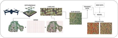
The labeled grids are divided into three subsets: training, validation, and testing. The training set is used to optimize the network parameters. The validation set is used to measure the performance of the model at each training epoch and to decide when to stop training. The test set is used to report metrics and evaluate the performance of the model on new unseen data. Following the partitions described in Section 2.2, our sets are composed by 243 images for training, 81 images for validation, and 81 images for testing (examples of the labels used to train the neural network models are shown in Figure 6). The general pipeline of the method is displayed in Figure 7.

Figure 7. General pipeline of the method presented in this work. The images are captured using the UAV and the orthomosaic is created. Grids are drawn in order to label portions of the image that are then used to train and evaluate the detection and semantic segmentation models.

2.4.1. Training

Deep neural networks usually need a large amount of annotated data to achieve their best performance. Also, the use of very few label data may produce overfitting. For that reason, we used data augmentation and fine-tuning approaches to improve generalization of our models.

Standard data augmentation techniques artificially augment the training data by applying random transformations to the input images and recomputing the new corresponding labels. In this work, we took advantage of the rotation-invariant property of our images. We used random flipping (using a probability of 0.5 both in the horizontal and vertical axis), random translation (sampled from a uniform distribution between $[-4,4]$ pixels both in horizontal and vertical directions), and rotations (sampling the rotation angle from a uniform probability distribution with values in $\{0,90,270\})$. Using this strategy, we are able to obtain up to 120 augmented versions from the same input image, obtaining a total of 29,160 training images. Applying these transformations it is unlikely that our model sees exactly the same image twice while training, helping to avoid overfitting.

Pretrained models from large-scale datasets have also demonstrated to be effective to avoid the overfitting (Yosinski et al. 2014). As the overall performance of object detection and instance segmentation algorithms are usually tested in the Common Objects in Context Dataset (COCO) (Lin et al. 2014), we used a pretrained Darknet neural network architecture for YOLO (Redmon and Farhadi 2018) and a pretrained Resnet-50 (He et al. 2016) for Mask R-CNN from this large-scale dataset to improve upon. We used the transfer learning technique named fine-tuning (Yosinski et al. 2014; Oquab et al. 2014) to optimize the entire network parameters over the entire pretrained network architectures. The best model was obtained by stopping the training when the evaluation over the validation set did not improve in mAP for more than 20 epochs. Both models were trained using the ADAM optimizer (Kingma and Ba 2015) with a learning rate of 0.001 both YOLO and Mask R-CNN.

Following these two simple approaches, we show that our models can produce highly accurate results from few labeled data.

2.4.2. Validation

Both YOLO and Mask R-CNN algorithms are aimed to identify the position of objects of interest in an image and metrics must be defined to validate their effectiveness.

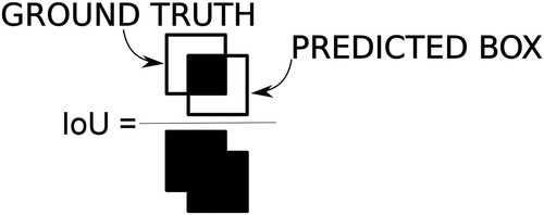
The basic measure for comparing two objects in an image is the Intersection Over Union (IoU). Between a predicted object and a ground truth label obtained by the visual inspection of the image (see Figure 6), we define the IoU as the division of the intersected area and the union of both areas (see Figure 8). For predictions that perfectly match the ground truth, the IoU value is 1; On the other hand, if both objects do not overlap, the IoU value is 0.

Figure 8. Intersection over union.

For a given threshold denoted as ε, IoU allows us to numerically evaluate the predictions of the model at localizing objects spatially. Identified objects that exceed the threshold are treated as true positives while remaining predictions are treated as false positives. Also, ground truth labels that does not match any prediction are treated as false negatives. Using these definitions, we can define precision and recall to evaluate the performance of the models. The precision metric is defined as (1) $\mathrm{p}\mathrm{r}\mathrm{e}\mathrm{c}\mathrm{i}\mathrm{s}\mathrm{i}\mathrm{o}\mathrm{n}=\frac{\mathrm{t}\mathrm{p}}{\mathrm{t}\mathrm{p}+\mathrm{f}\mathrm{p}},$(1) where tp are the true positives and fp are the false positives. This represents the ratio between the number of correctly predicted objects and the total number of predicted objects. In a similar way we define the recall as (2) $\mathrm{r}\mathrm{e}\mathrm{c}\mathrm{a}\mathrm{l}\mathrm{l}=\frac{\mathrm{t}\mathrm{p}}{\mathrm{t}\mathrm{p}+\mathrm{f}\mathrm{n}},$(2) where fn are the false negatives. This metric represents the ratio between the number of correctly predicted objects and the total number of true objects (ground truth).

Using the precision and recall metrics we define the Average Precision (AP) as main value to be used in the validation of the model. This metric is a standard measure of the quality in object detection and semantic segmentation. It is defined as the area under the precision-recall curve $p\left(r\right)$, sorted by confidence prediction values (Everingham et al. 2010). Formally, the AP for a given threshold is defined as (3) ${\mathrm{A}\mathrm{P}}_{ϵ}={\int }_0^{1}p\left(r\right)\mathrm{d}r.$(3)

We integrate the precision-recall curve over the detection threshold r. Due to variations produced when sorting by confidence, usually a zigzag pattern is shown in the curve $p\left(r\right)$. We avoid this by using, instead, the max precision ‘to the right’ of that recall level, meaning that we replace p with $p_{ip}\left(r\right)=\underset{\tilde{r}\ge r}{max}p\left(\tilde{r}\right)$.

Similar to popular contents for objects detection and instance segmentation like PASCAL VOC (Everingham et al. 2010), we fix $ϵ=0.5$ as the standard threshold value to compute all our results. It is worth noting that this value can be changed and metrics should vary. However, this decision depends on the precision needed to overcome the identification task. When the spatial locations of the object of interest are not required, this task becomes counting and is the same as defining $ϵ=0$.

To select the hyperparameters, we computed the averaged the ${\mathrm{A}\mathrm{P}}_{0.5}^{\left(i\right)}$ value over all the N = 81 images in the validation set as ${\mathrm{m}\mathrm{A}\mathrm{P}}_{0.5}=\sum _{i=1}^N{\mathrm{A}\mathrm{P}}_{0.5}^{\left(i\right)}$. Training process is stopped when the ${\mathrm{m}\mathrm{A}\mathrm{P}}_{0.5}$ measured over the validation set does not improve for more than 15 epochs.

2.5. Evaluation

The goal of our work is to detect different trees in a complete field. Due to the size of these fields, we cannot obtain its characterization directly from a single image. The trivial division of a field image to obtain the total number of trees by adding the contributions of each sub-image will introduce detection errors in the boundaries of these images, either because it will be harder for the neural network to detect incomplete labels or because one can double the detection of a single tree.

Following the procedure described in Section 2.2, we propose an assembly for the detected overlapped sub-images that can account for boundary problems. The idea is to reconstruct a global prediction by merging the predictions of the centers of each sub-image. By doing so, we only take into consideration predictions whose center is within the boundaries of the center of each sub-image. In Figure 9, we depicted the aforementioned procedure to merge the predictions. Using this merged image and the respective labels, we are able to compute metrics for evaluation.

Figure 9. Each square has $32\times 32$ pixels. (a) Thick square: First subimage given to neural network, and output with centroid in blue the section considered. (b) Thick square: Second subimage given to neural network, in blue the section considered. In red the section considered in the last step (c) In red all the area that was considered in the end of the process.

3. Results

We compared the presented algorithms in three tasks: counting, detection, and segmentation. These tasks are similar but differ in how the predictions are evaluated. Specifically, for detection and segmentation an IoU's threshold $ϵ=0.5$ is used to evaluate the match between predictions and ground truths spatially (see Section 2.4.2 for details). As spatial locations are not needed for counting, all the model predictions are used for evaluation.

3.1. Counting

Counting is useful when spatial locations are not needed as an objective task (e.g. to estimate the number of trees that survived after being planted). Therefore, the relevant values are the number of trees, rather than their positions in the space. We compare the algorithms YOLO and Mask R-CNN for the counting task. Each algorithm is evaluated over the test subset defined for each forest stand (it is worth noting that the test subsets are not used for training, but only for evaluation purposes). As can be seen in Table 2, both models achieve lower than $15\text{\%}$ of relative error for both algorithms. The averaged relative error for all the forest stands using YOLO is $8.5\text{\%}$ while using Mask R-CNN is $4.7\text{\%}$.

Table 2. YOLO and Mask R-CNN results for the task of counting forest stands of different ages. diff indicates relative difference between the predictions and the ground truth. Negative values denote underestimation, while positive values denote overestimation. Average indicates the mean absolute values of the percentage difference.

	YOLO		Mask R-CNN
Age (years)	Count	diff ($\text{\%}$)	Count	diff ($\text{\%}$)	Ground truth
1	62	$-6.0$	64	$-3.0$	66
5	169	$-5.0$	191	$+7.3$	178
8	79	$+12.8$	76	$-8.6$	70
10	149	$-10.2$	166	0.0	166
Average		8.5		4.7

Although the older trees, therefore the denser stands, are expected to be more difficult to detect, the opposite result was obtained in the case of Mask R-CNN: the older the trees, the better the obtained results are. On the other hand, we observe that YOLO achieves bad results for older forest stands (8 and 10 years). This is due to the overlapping of the tree tops, which makes their detection difficult using YOLO. In Section 4 we provide some insights about this behavior.

3.2. Detection

Detection is appropriate when spatial locations are important for the task (e.g. to estimate where are the trees that survived after being planted). Unlike the counting task, in detection we expect to match the predictions of the algorithm with the spatial location of the trees. For that reason, an IoU threshold criteria of $ϵ=0.5$ is used to evaluate this task (see Section 2.4.2 for details). When the Iou between the prediction and the ground truth exceeds the threshold, the prediction is considered as a true positive sample. On the other hand, when the threshold is not exceeded, predicted values are treated as false positives (i.e. predictions that that do not meet the IoU criteria or that does not match the ground truth spatially), and the unmatched ground truth labels are treated as false negatives (i.e. true labels that were not detected). The results for tree detection using the YOLO and Mask R-CNN algorithms are shown in Tables 3 and 4. We observe that Mask R-CNN performs better than YOLO in most of the cases in terms of the ${\mathrm{A}\mathrm{P}}_{0.5}$. Also, Mask R-CNN's average ${\mathrm{A}\mathrm{P}}_{0.5}$ is considerably higher than YOLO's.

Table 3. YOLO results for the task of detecting forest stands of different ages. We denote true positive (TP), false positive (FP), and false negative (FN).

	YOLO
Age (years)	Precision	Recall	F1-Score	TP	FP	FN	${\mathrm{A}\mathrm{P}}_{0.5}$
1	0.63	0.59	0.61	39	23	27	0.56
5	0.74	0.65	0.69	125	44	66	0.64
8	0.87	0.91	0.89	69	10	7	0.85
10	0.62	0.55	0.58	92	57	74	0.38
Average	0.72	0.68	0.69				0.61

Table 4. Mask R-CNN results for the task of detecting forest stands of different ages.

	Mask R-CNN
Age (years)	Precision	Recall	F1-Score	TP	FP	FN	${\mathrm{A}\mathrm{P}}_{0.5}$
1	0.75	0.73	0.74	48	16	18	0.70
5	0.84	0.78	0.81	150	28	41	0.81
8	0.86	0.79	0.82	60	10	16	0.82
10	0.92	0.92	0.92	153	13	13	0.91
Average	0.82	0.80	0.82				0.81

Better results for Mask R-CNN were consistently obtained as the age of the trees increased, while results for YOLO decreased in that case. This poor performance of YOLO is due to a large amount of overlapping presented in the 5 and 10-year-old forest stands, which generates confusion that does not allow the model to match the predictions and labels spatially.

The deterioration of the models in detection may seem surprising given their good results in the counting task. As will be explained in detail in Section 4, this behavior is due to the threshold used to report metrics. Most false positives and false negatives correspond to detections that do not exceed the threshold criterion, so it is important to note that the reported metrics are designed for accurate detection.

3.3. Segmentation

When we add the segmentation to the detection task we obtain instance segmentation. This task is useful when differences between the size of the tree in different periods are needed (e.g. to estimate how much a tree or group of trees has grown in the last period).

Even though YOLO is not meant to perform well in instance segmentation, we use the predicted bounding boxes to estimate the area of the tree crowns and we compare against Mask R-CNN predictions. Specifically, for YOLO we used the number of pixels inside of the predicted bounding boxes to estimate the areas of the trees. In case of overlapping between two bounding boxes, we consider the union once. For Mask R-CNN, we use the number of the segmented pixels of the predictions to estimate the tree areas. Table 5 shows the predicted areas for each of the forest stand, measured in square meters (m${}^2$). As can be seen, the averaged relative difference between the areas predicted by Mask R-CNN is lower than the predicted by YOLO. Despite this, the averaged relative difference does is lower than $15\text{\%}$. Therefore, it is considered that the YOLO results are quite competitive for detecting one and five-year-old trees.

Table 5. YOLO and Mask R-CNN results for the task of segmentating forest stands of different ages. Average indicates the mean absolute values of the percentage difference.

	YOLO		Mask R-CNN
Age (years)	Area (m${}^2$)	diff ($\text{\%}$)	Area (m${}^2$)	diff ($\text{\%}$)	Ground truth
1	56	$-3.4$	52	$-6.9$	58
5	785	$-24.9$	841	$-19.6$	1, 046
8	606	$+5.0$	580	$+0.5$	577
10	1, 520	$-20.7$	1, 730	$-9.8$	1, 918
Average		13.5		9.2

4. Discussion

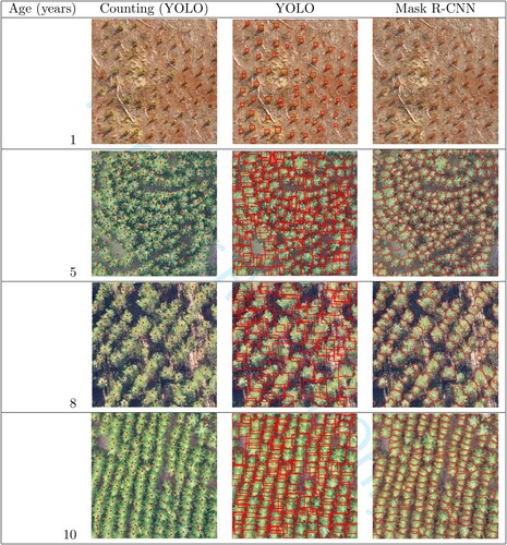
To analyze the predictions, Figure 10 shows the predictions for counting and detection produced by YOLO, and the segmented masks produced by Mask R-CNN. As can be seen, the size and overlap between trees increase as they become older. For the YOLO algorithm, best results were obtained for small trees rather than highly overlapped forest stands. In contrast, Mask R-CNN tends to achieve better results in presence of high overlapping rather than smaller stands. These findings agrees with findings made in previous works (Drid, Allaoui, and Kherfi 2020; Wu et al. 2021; Machefer et al. 2020).

Figure 10. Predictions of the counting (YOLO), detection, and segmentation (Mask R-CNN) tasks for each of the forest stands.

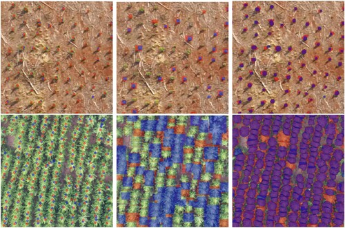
To understand the limitations of the proposed methods, we visualize predictions and ground truth labels for the one and ten year old forest stands in Figure 11. We chose these stands as they contains the areas with the lowest and highest density of trees, respectively. The first column shows the YOLO results for counting. As can be seen, this model generates predictions that coincide with the ground truth of the forest stands. However, when we change to the detection task, the IoU threshold causes some of these objects to become false positives (Redmon et al. 2016). This behavior is displayed in the second column. In this figure, detections that do not meet the IoU criteria are drawn with filled blue squares, and labels that does not match any prediction are drawn with filled red squares. Despite the majority of these predictions coincide with their respective ground truth, some of them are considered as false positive detections due to the high overlapping with neighboring trees. One can think that the metrics can be improved by varying the IoU threshold, but the decision depends on the precision required to overcome the identification task. In the case of segmentation, the third column shows that Mask R-CNN segments bigger trees with greater precision than younger trees. This behavior can be explained by labels size, that in some cases are smaller than the fixed convolutional kernel sizes of the pretrained Mask R-CNN architecture (He et al. 2017), making difficult for the neural network to detect these cases.

Figure 11. Predictions for the one and ten years old forest stands (in blue), contrasted with the ground truth (in red). The first row shows the results for the one year old forest stand, while the second row for the ten years old forest stand.

5. Conclusion and future work

Despite the difficulties given by the constant monitoring of trees, deep neural network models can be used to automate this process. In this work, we compared two deep neural network methods to evaluate their effectiveness for automatic monitoring of forests. Specifically, we used YOLO and Mask R-CNN for the counting, detection, and segmentation tasks of pine cultivations of different ages and densities using RGB images taken from UAVs. We propose a methodology to train and evaluate the models using high-dimensional images and we show the effectiveness of the proposed methods. Our results suggest that both methods are able to deal with the counting, detection, and segmentation tasks. For the counting task, YOLO overestimates $8.5\text{\%}$ of the detected trees in average, whereas Mask R-CNN overestimates an $4.7\text{\%}$ of the detected trees in average. For the detection task, YOLO obtains a precision of 0.72 and a recall of 0.68 in average, while Mask R-CNN obtains a precision of 0.82 and a recall of 0.80 in average. In the segmentation task, YOLO overestimates an $13.5\text{\%}$ of the predicted area in average, whereas mask overestimates a $9.2\text{\%}$ of the predicted area in average.

Furthermore, the proposed methods presents a cost-effective solution for forest monitoring using RGB airborne imagery.

For future work we expect to implement and compare our methods with the new generation of real-time detection and object segmentation algorithms Scaled YOLO v4 (Wang, Bochkovskiy, and Liao 2021), YOLO v7 (Wang, Bochkovskiy, and Liao 2022), and YOLACT (Bolya et al. 2020). Using these algorithms we expect to obtain significant performance improvements. Additionally, we expect to make an extensive analysis of the inference time of the presented algorithms under different hardware conditions.

Acknowledgements

We acknowledge Forestal Arauco S.A. for funding, to the Planning Management team for the acquisition of field data and flight images with UAVs, and to Rodrigo Sobarzo and Fernando Bustamante for their support to the project. We acknowledge support from FONDEF IDeA I+D 2021 ID21I10354. GCV acknowledges support from FONDECYT Initiation Nº 11191130.No potential competing interest was reported by the authors.

Disclosure statement

No potential conflict of interest was reported by the author(s).

Data availability statement

The data that support the findings of this study are available from the corresponding author, M. Perez-Carrasco, upon reasonable request.

Notes

1 https://www.dronedeploy.com/.

References

- Abadi, Martín, Ashish Agarwal, Paul Barham, Eugene Brevdo, Zhifeng Chen, Craig Citro, and Greg S. Corrado, et al. 2015. “TensorFlow: Large-Scale Machine Learning on Heterogeneous Systems.” Software available from tensorflow.org, https://www.tensorflow.org/.
- Ampatzidis, Yiannis, and Victor Partel. 2019. “UAV-Based High Throughput Phenotyping in Citrus Utilizing Multispectral Imaging and Artificial Intelligence.” Remote Sensing 11 (4): 410.
- Bolya, Daniel, Chong Zhou, Fanyi Xiao, and Yong Jae Lee. 2020. “YOLACT++: Better Real-Time Instance Segmentation.” IEEE Transactions on Pattern Analysis and Machine Intelligence
- Csillik, Ovidiu, John Cherbini, Robert Johnson, Andy Lyons, and Maggi Kelly. 2018. “Identification of Citrus Trees From Unmanned Aerial Vehicle Imagery Using Convolutional Neural Networks.” Drones2 (4): 39.
- Dai, Jifeng, Kaiming He, and Jian Sun. 2016. “Instance-Aware Semantic Segmentation Via Multi-Task Network Cascades.” In Proceedings of the IEEE Conference on Computer Vision and Pattern Recognition, 3150–3158.
- Drid, Khaoula, Mebarka Allaoui, and Mohammed Lamine Kherfi. 2020. “Object Detector Combination for Increasing Accuracy and Detecting More Overlapping Objects.” In Image and Signal Processing, edited by Abderrahim El Moataz, Driss Mammass, Alamin Mansouri, and Fathallah Nouboud, Cham, 290–296. Springer International Publishing.
- Everingham, M., L. Van Gool, C. K. I. Williams, J. Winn, and A. Zisserman. 2010. “The Pascal Visual Object Classes (VOC) Challenge.” International Journal of Computer Vision 88 (2): 303–338.
- Fricker, Geoffrey A, Jonathan D Ventura, Jeffrey A Wolf, Malcolm P North, Frank W Davis, and Janet Franklin. 2019. “A Convolutional Neural Network Classifier Identifies Tree Species in Mixed-Conifer Forest From Hyperspectral Imagery.” Remote Sensing 11 (19): 2326.
- Fukushima, Kunihiko. 1980. “Neocognitron: A Self-organizing Neural Network Model for a Mechanism of Pattern Recognition Unaffected by Shift in Position.” Biological Cybernetics 36: 193–202.
- Graves, Sarah J, Gregory P Asner, Roberta E Martin, Christopher B Anderson, Matthew S Colgan, Leila Kalantari, and Stephanie A Bohlman. 2016. “Tree Species Abundance Predictions in a Tropical Agricultural Landscape with a Supervised Classification Model and Imbalanced Data.” Remote Sensing8 (2): 161.
- Hartling, Sean, Vasit Sagan, Paheding Sidike, Maitiniyazi Maimaitijiang, and Joshua Carron. 2019. “Urban Tree Species Classification Using a WorldView-2/3 and LiDAR Data Fusion Approach and Deep Learning.” Sensors 19 (6): 1284.
- Hassaan, Omair, Ahmad Kamal Nasir, Hubert Roth, and M. Fakhir Khan. 2016. “Precision Forestry: Trees Counting in Urban Areas Using Visible Imagery Based on An Unmanned Aerial Vehicle.” IFAC-PapersOnLine 49 (16): 16–21.
- He, Kaiming, Georgia Gkioxari, Piotr Dollár, and Ross Girshick. 2017. “Mask R-CNN.” In Proceedings of the IEEE International Conference on Computer Vision, 2961–2969.
- He, Kaiming, Xiangyu Zhang, Shaoqing Ren, and Jian Sun. 2016. “Deep Residual Learning for Image Recognition.” In Proceedings of the IEEE Conference on Computer Vision and Pattern Recognition, 770–778.
- Johnson, Jeremiah W. 2018. Adapting Mask-RCNN for Automatic Nucleus Segmentation. arXiv preprint arXiv:1805.00500.
- Katoh, Masato, and François A. Gougeon. 2012. “Improving the Precision of Tree Counting by Combining Tree Detection with Crown Delineation and Classification on Homogeneity Guided Smoothed High Resolution (50 Cm) Multispectral Airborne Digital Data.” Remote Sensing 4 (5): 1411–1424.
- Kingma, Diederik P., and Jimmy Ba. 2015. “Adam: A Method for Stochastic Optimization.” In 3rd International Conference on Learning Representations, ICLR 2015, San Diego, CA, USA, May 7–9, 2015, Conference Track Proceedings, edited by Yoshua Bengio and Yann LeCun. http://arxiv.org/abs/1412.6980.
- Lange, Sven, Niko Sünderhauf, Peer Neubert, Sebastian Drews, and Peter Protzel. 2012. “Autonomous Corridor Flight of a UAV Using a Low-Cost and Light-Weight RGB-D Camera.” In Advances in Autonomous Mini Robots, 183–192. Springer.
- Lecun, Yann, Leon Bottou, Y. Bengio, and Patrick Haffner. 1998. “Gradient-Based Learning Applied to Document Recognition.” Proceedings of the IEEE 86: 2278–2324.
- Li, Yi, Haozhi Qi, Jifeng Dai, Xiangyang Ji, and Yichen Wei. 2017. “Fully Convolutional Instance-Aware Semantic Segmentation.” In Proceedings of the IEEE Conference on Computer Vision and Pattern Recognition, 2359–2367.
- Lin, Tsung-Yi, Michael Maire, Serge Belongie, James Hays, Pietro Perona, Deva Ramanan, Piotr Dollár, and C. Lawrence Zitnick. 2014. “Microsoft COCO: Common Objects in Context.” In Computer Vision – ECCV 2014, edited by David Fleet, Tomas Pajdla, Bernt Schiele, and Tinne Tuytelaars, Cham, 740–755. Springer International Publishing.
- Long, Jonathan, Evan Shelhamer, and Trevor Darrell. 2014. Fully Convolutional Networks for Semantic Segmentation. CoRR abs/1411.4038. http://arxiv.org/abs/1411.4038.
- Ma, Lei, Yu Liu, Xueliang Zhang, Yuanxin Ye, Gaofei Yin, and Brian Alan Johnson. 2019. “Deep Learning in Remote Sensing Applications: A Meta-analysis and Review.” ISPRS Journal of Photogrammetry and Remote Sensing 152: 166–177.
- Machefer, Mélissande, François Lemarchand, Virginie Bonnefond, Alasdair Hitchins, and Panagiotis Sidiropoulos. 2020. “Mask R-CNN Refitting Strategy for Plant Counting and Sizing in UAV Imagery.” Remote Sensing 12 (18): 3015.
- Marques, Pedro, Luís Pádua, Telmo Ad ao, Jonáš Hruška, Emanuel Peres, António Sousa, and Joaquim J Sousa. 2019. “UAV-based Automatic Detection and Monitoring of Chestnut Trees.” Remote Sensing 11 (7): 855.
- Onishi, Masanori, and Takeshi Ise. 2021. “Explainable Identification and Mapping of Trees Using UAV RGB Image and Deep Learning.” Scientific Reports 11:
- Oquab, M., L. Bottou, I. Laptev, and J. Sivic. 2014. “Learning and Transferring Mid-level Image Representations Using Convolutional Neural Networks.” In 2014 IEEE Conference on Computer Vision and Pattern Recognition, 1717–1724.
- Panteleris, Paschalis, Iason Oikonomidis, and Antonis Argyros. 2018. “Using a Single RGB Frame for Real Time 3D Hand Pose Estimation in the Wild.” In 2018 IEEE Winter Conference on Applications of Computer Vision (WACV), 436–445. IEEE.
- Paoletti, Mercedes E, Juan Mario Haut, Javier Plaza, and Antonio Plaza. 2018. “A New Deep Convolutional Neural Network for Fast Hyperspectral Image Classification.” ISPRS Journal of Photogrammetry and Remote Sensing 145: 120–147.
- Park, Tae-Jin, Jong-Yeol Lee, Woo-Kyun Lee, Doo-Ahn Kwak, Han-Bin Kwak, and Sang-Chul Lee. 2011. “Automated Individual Tree Detection and Crown Delineation Using High Spatial Resolution RGB Aerial Imagery.” Korean Journal of Remote Sensing 27 (6): 703–715.
- Paszke, Adam, Sam Gross, Francisco Massa, Adam Lerer, James Bradbury, Gregory Chanan, and Trevor Killeen, et al. 2019. “Pytorch: An Imperative Style, High-Performance Deep Learning Library.” In Advances in Neural Information Processing Systems, 8026–8037.
- Poblete-Echeverría, Carlos, Guillermo Federico Olmedo, Ben Ingram, and Matthew Bardeen. 2017. “Detection and Segmentation of Vine Canopy in Ultra-High Spatial Resolution RGB Imagery Obtained From Unmanned Aerial Vehicle (UAV): A Case Study in a Commercial Vineyard.” Remote Sensing 9 (3): 268.
- Pouliot, D. A., D. J. King, F. W. Bell, and D. G. Pitt. 2002. “Automated Tree Crown Detection and Delineation in High-Resolution Digital Camera Imagery of Coniferous Forest Regeneration.” Remote Sensing of Environment 82 (2–3): 322–334.
- QGIS Development Team. 2022. QGIS Geographic Information System. QGIS Association. url https://www.qgis.org.
- Redmon, Joseph, Santosh Divvala, Ross Girshick, and Ali Farhadi. 2016. “You Only Look Once: Unified, Real-Time Object Detection.” In Proceedings of the IEEE Conference on Computer Vision and Pattern Recognition, 779–788.
- Redmon, Joseph, and Ali Farhadi. 2018. Yolov3: An Incremental Improvement. arXiv preprint arXiv:1804.02767.
- Ren, Shaoqing, Kaiming He, Ross Girshick, and Jian Sun. 2015. “Faster R-CNN: Towards Real-Time Object Detection with Region Proposal Networks.” In Advances in Neural Information Processing Systems, 91–99.
- Ronneberger, Olaf, Philipp Fischer, and Thomas Brox. 2015. “U-Net: Convolutional Networks for Biomedical Image Segmentation.” CoRR abs/1505.04597. http://arxiv.org/abs/1505.04597.
- Santoro, Franco, Eufemia Tarantino, Benedetto Figorito, Stefania Gualano, and Anna Maria D'Onghia. 2013. “A Tree Counting Algorithm for Precision Agriculture Tasks.” International Journal of Digital Earth 6 (1): 94–102.
- Surovỳ, Peter, Nuno Almeida Ribeiro, and Dimitrios Panagiotidis. 2018. “Estimation of Positions and Heights From UAV-Sensed Imagery in Tree Plantations in Agrosilvopastoral Systems.” International Journal of Remote Sensing 39 (14): 4786–4800.
- Wallace, Luke, Robert Musk, and Arko Lucieer. 2014. “An Assessment of the Repeatability of Automatic Forest Inventory Metrics Derived From UAV-Borne Laser Scanning Data.” IEEE Transactions on Geoscience and Remote Sensing 52 (11): 7160–7169.
- Wang, Chien-Yao, Alexey Bochkovskiy, and Hong-Yuan Mark Liao. 2021. “Scaled-YOLOv4: Scaling Cross Stage Partial Network.” In Proceedings of the IEEE/CVF Conference on Computer Vision and Pattern Recognition (CVPR), June, 13029–13038.
- Wang, Chien-Yao, Alexey Bochkovskiy, and Hong-Yuan Mark Liao. 2022. YOLOv7: Trainable Bag-of-Freebies Sets New State-of-the-Art for Real-Time Object Detectors. arXiv preprint arXiv:2207.02696.
- Wang, Jiamin, Xinxin Chen, Lin Cao, Feng An, Bangqian Chen, Lianfeng Xue, and Ting Yun. 2019. “Individual Rubber Tree Segmentation Based on Ground-Based LiDAR Data and Faster R-CNN of Deep Learning.” Forests 10 (9): 793.
- Wu, Qifan, Daqiang Feng, Changqing Cao, Xiaodong Zeng, Zhejun Feng, Jin Wu, and Ziqiang Huang. 2021. “Improved Mask R-CNN for Aircraft Detection in Remote Sensing Images.” Sensors 21 (8): 2618.
- Wulder, Mike, K. Olaf Niemann, and David G. Goodenough. 2000. “Local Maximum Filtering for the Extraction of Tree Locations and Basal Area From High Spatial Resolution Imagery.” Remote Sensing of Environment 73 (1): 103–114.
- Yosinski, Jason, Jeff Clune, Yoshua Bengio, and Hod Lipson. 2014. “How Transferable are Features in Deep Neural Networks?” In Advances in Neural Information Processing Systems, edited by Z. Ghahramani, M. Welling, C. Cortes, N. Lawrence, and K. Q. Weinberger, Vol. 27, 3320–3328. Curran Associates, Inc. https://proceedings.neurips.cc/paper/2014/file/375c71349b295fbe2dcdca9206f20a06-Paper.pdf.
- Zhang, Liangpei, Lefei Zhang, and Bo Du. 2016. “Deep Learning for Remote Sensing Data: A Technical Tutorial on the State of the Art.” IEEE Geoscience and Remote Sensing Magazine 4 (2): 22–40.
- Zhao, Tiebiao, Yonghuan Yang, Haoyu Niu, Dong Wang, and YangQuan Chen. 2018. “Comparing U-Net Convolutional Network with Mask R-CNN in the Performances of Pomegranate Tree Canopy Segmentation.” In Multispectral, Hyperspectral, and Ultraspectral Remote Sensing Technology, Techniques and Applications VII, Vol. 10780, 107801J. International Society for Optics and Photonics.