An improvement of snow/cloud discrimination from machine learning using geostationary satellite data

ABSTRACT

Snow and cloud discrimination is a main factor contributing to errors in satellite-based snow cover. To address the error, satellite-based snow cover performs snow reclassification tests on the cloud pixels of the cloud mask, but the error still remains. Machine Learning (ML) has recently been applied to remote sensing to calculate satellite-based meteorological data, and its utility has been demonstrated. In this study, snow and cloud discrimination errors were analyzed for GK-2A/AMI snow cover, and ML models (Random Forest and Deep Neural Network) were applied to accurately distinguish snow and clouds. The ML-based snow reclassified was integrated with the GK-2A/AMI snow cover through post-processing. We used the S-NPP/VIIRS snow cover and ASOS in situ snow observation data, which are satellite-based snow cover and ground truth data, as validation data to evaluate whether the snow/cloud discrimination is improved. The ML-based integrated snow cover detected 33–53% more snow compared to the GK-2A/AMI snow cover. In terms of performance, the F1-score and overall accuracy of the GK-2A/AMI snow cover was 73.06% and 89.99%, respectively, and those of the integrated snow cover were 76.78–78.28% and 90.93–91.26%, respectively.

KEYWORDS:

• Geostationary satellite
• GK-2A/AMI snow cover product
• snow/cloud discrimination
• machine learning
• remote sensing

1. Introduction

Snow plays a vital role in regulating heat flow between the Earth’s surface and the atmosphere and the global radiative energy balance, owing to its high albedo and low thermal conductivity (Bair, Davis, and Dozier 2018; Cohen and Rind 1991; Domine et al. 2015; Groisman, Karl, and Knight 1994). Its environmental impact is wide ranging, encompassing ecosystems, drought hazards, and agriculture (Biemans et al. 2019; Musselman et al. 2017). Thus, accurate Snow Cover (SC) observation is essential for monitoring climate change and environmental conditions at the local level (Croce et al. 2018).

Satellite data–based observation is the most effective method of monitoring snow cover (Liu et al. 2020), and most Earth observation satellites produce snow cover (Hall and Salomonson 2006; Key et al. 2013, 2020; Muhuri et al. 2021). The Korea Meteorological Administration (KMA) also produces snow cover using the Advanced Meteorological Imager (AMI) onboard the GEO-KOMPSAT-2A (GK-2A) (Han, Jin, and Lee 2019). Satellite-based snow cover are used to investigate environmental factors that affect human life, design infrastructure for use in cold climates, understand climate variability and change, and improve weather forecasting (Key et al. 2013). The use of operational satellite-based snow cover across various fields thus elevates the importance of accuracy in its production.

Most operational satellite-based snow cover use a cloud mask algorithm as auxiliary data. The snow cover detection algorithm uses the cloud mask to detect snow cover pixels that are not polluted by cloud (Key et al. 2020, 2013; Siljamo and Hyvärinen 2011). Accordingly, the algorithm is structurally affected by the cloud mask used as input data. If the cloud mask detects a snow area as cloud, the snow cover algorithm excludes the corresponding area from the potential snow area. To improve the uncertainty, satellite-based snow cover needs to be reclassified and post-processed for pixels masked by clouds.

A traditional method is threshold method that uses different combinations of channels to discriminate between snow and cloud has gained traction in recent years. In particular, the short-wave infrared (SWIR) band and Normalized Difference Snow Index (NDSI) is widely used to discriminate between snow and cloud (Dozier 1989; Hall, Riggs, and Salomonson 1995; Härer et al. 2018; Warren 1982). However, the snow and cloud reflectance used in the threshold method is significantly affected by multiple factors (King et al. 1997; Platnick et al. 2003; Xie et al. 2006; Zhu, Wang, and Woodcock 2015). Due to this feature, threshold-based snow cover has potential uncertainty. In this reason, the key contributing factor to uncertainty in snow cover is inaccurate discrimination between snow and cloud (Riggs and Hall 2004; Zhu and Woodcock 2012, 2014). Lee et al. (2017) performed snow mapping including snow cover and cloud classification by using the Dynamic Wavelength Warping (DWW) method that considered the reflectance variability of snow cover. The snow cover of GK-2A/AMI, a geostationary satellite with a high temporal resolution of 10 min, also reclassified the snow cover for cloud pixels by using the DWW method that considers the reflectance variability of the snow cover (Han, Jin, and Lee 2019). Despite these efforts, there are areas in the GK-2A/AMI snow cover that cannot reclassify the actual snow cover into snow cover. For this reason, post-processing is required to correctly reclassify the pixels classified as clouds as snow cover, which is an actual snow area.

The use of machine learning (ML) has increased in the field of remote sensing (Choi et al. 2021; Yang et al. 2022; Rodriguez-Galiano and Chica-Rivas 2014; Wang, Zhong, and Ma 2022), and is also widely used for snow, cloud detection (De Gregorio et al. 2019; Cannistra, Shean, and Cristea 2021; Luo et al. 2022; Miller et al. 2018) and snow/cloud discrimination (Varshney et al. 2018; Xia et al. 2019; Zhan et al. 2017). Most of the snow/cloud discrimination studies using ML focused on verifying the performance of ML through comparison with the traditional snow/cloud discrimination methods. Although ML has higher accuracy in distinguishing snow and cloud than traditional methods, the long-term and stable use of snow/cloud discrimination using ML has not been proven. In addition, most of the snow/cloud discrimination studies through machine learning used polar orbit satellite (Varshney et al. 2018; Xia et al. 2019; Zhan et al. 2017), and studies on snow/cloud discrimination using geostationary meteorological satellites were insufficient. A geostationary meteorological satellite-based snow cover with high temporal resolution enables detailed snow distribution monitoring than a polar-orbit satellite-based snow cover. The purpose of this study is to evaluate the performance of ML for snow cover and cloud classification and to improve the uncertainty of snow cover by performing snow reclassification through ML for the cloud area among the geostationary satellite GK-2A/AMI snow cover. The remainder of this paper proceeds as follows. Section 2 describes the study data study areas. Section 3 describes the snow/cloud discrimination methods of this study. Section 4 presents the study results. Section 5 discusses the study results. Section 6 presents the conclusions.

2. Study area and data

2.1. Study area and GK-2A/AMI data

Our study area was the Full-Disk (FD) observation area of the geostationary meteorological satellite GK-2A/AMI (Figure 1). GK-2A/AMI was launched in December 2019, succeeding Communication, Ocean and Meteorological Satellite/Meteorological Imager and performing meteorological and space weather observation missions as a geostationary meteorological satellite for KMA. For the FD observation area of GK-2A/AMI, the temporal resolution is 10 min, and the spatial resolution is 500 m, 1 km, or 2 km, depending on the channel data. The area covers the Himalayas, which are a frequent site of icecap and snow cover monitoring studies (Chaujar 2009; Thompson et al. 2006; Hao et al. 2019). In addition, snow cover is widely distributed in north-eastern Asia and eastern Eurasia during the northern hemisphere winter, and snow studies are ongoing in the region (Qiao and Wang 2019; You et al. 2020; Zhang and Ma 2018).

Figure 1. Study area on the GK-2A/AMI full disk.

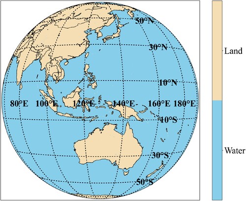
The study period was from January to March 2020 – the northern hemisphere winter, when the study area receives abundant snow – to facilitate the collection of sufficient training and test data. The GK-2A/AMI data used as input data for ML models for snow/cloud discrimination included top of atmosphere (TOA) channel data, latitude data. The GK-2A/AMI bands we used comprised four TOA reflectance bands (one visible multispectral band, one near infrared [NIR] multispectral band, and two SWIR multispectral bands) and three TOA brightness temperature bands (three infrared [IR] multispectral bands). When using TOA channel data, we changed all spatial resolutions that differed for each channel to 2 km. The GK-2A/AMI snow cover product – the target data for discriminating between snow and cloud to which ML was applied – has a spatial resolution of 2 km, and temporal resolution is provided in the form of 10-min and 1-day data. The accuracy with which it discriminates between snow and snow-free land is high, as precision is 97.14% and recall is 1.96% (Han, Jin, and Lee 2019). We used the GK-2A/AMI snow cover product, which is provided every 10 min. GK-2A/AMI true-color RGB and snow–fog RGB images were used for qualitative validation of the model results. Snow–fog RGB images provide optimal color contrast between snow/ice-covered surfaces and water cloud/fog during the daytime. Therefore, it is easy to distinguish between snow and cloud, which are difficult to distinguish in true-color RGB images. The true-color RGB images were used not only to discriminate between snow and cloud but also to distinguish snow/cloud from snow-free land.

2.2. S-NPP/VIIRS snow cover product

The Suomi-NPP/Visible Infrared Imager Radiometer Suite (VIIRS) snow cover product with a temporal resolution of approximately every 12 h and a nominal pixel spatial resolution of 375 m was used as reference data and validation data for snow/cloud discrimination. This data is a swath product, and ‘NDSI Snow Cover’ data from the dataset was used. Compared to the Moderate Resolution Imaging Spectroradiometer (MODIS) snow cover product, the S-NPP/VIIRS snow cover product has an accuracy of 88–93% (Riggs, Hall, and Román 2016). The S-NPP/VIIRS snow cover product removes the cloud-contaminated area using the S-NPP/VIIRS cloud mask as precedent data and then detects snow cover in the remaining area. Accordingly, the data include not only snow but also cloud information, and we used the corresponding snow and cloud information. The S-NPP/VIIRS snow cover product provides a quality flag, and we used only high-quality data with a Solar Zenith Angle (SZA) of less than 70°.

2.3. ASOS in situ snow observation data

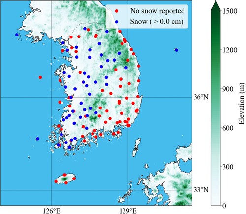
The Automated Synoptic Observing System (ASOS) data produced by KMA provides air temperature, precipitation, visibility, snow depth and so on. In remote sensing, ASOS data is used as verification data to evaluate the performance of meteorological products (Lee et al. 2017; Choi et al. 2021). We validated the snow detection performance by using ASOS snow data, a snow depth in situ observation system for the final snow cover whose snow/cloud discrimination was improved by ML. We collected ASOS daily snowfall amounts from January to March 2020, 2021, through the KMA meteorological data portal (available at https://data.kma.go.kr/data/grnd/selectAsosRltmList.do?pgmNo=36) for 140 snow depth observation stations in South Korea. Figure 2 shows the snow area according to ASOS daily snowfall amounts at 04:00 UTC on 17 February 2020, along with the stations for which snow depth was not reported.

Figure 2. Spatial distribution of 140 stations in South Korea and information on ASOS in situ snow observation data (17 February 2020, 04:00 UTC).

3. Methods

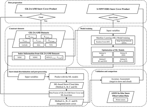
Figure 3 is the research process for snow/cloud discrimination using GK-2A/AMI data via ML in this study. The research process consists of a total of five steps. The first process is the data preparation stage, and the GK-2A/AMI dataset and S-NPP/VIIRS snow cover data were collected from January 2020 to March 2021. The second process is the step of constructing an input data set for driving ML. The third process is training the ML models (RF and DNN). The fourth step is to reclassify the actual snow cover area among the cloud areas through four methods (Method A, B, C, D) based on ML models. We defined the method using the RF model in the snow/cloud discrimination process as Method A and the method using the DNN model as Method B. Method C is snow/cloud discrimination process to classify the pixel as snow when both RF-based data and DNN-based data for a specific pixel are classified as snow. Lastly, If any one of the two models (RF and DNN) was classified as an snow, the process of classifying the corresponding pixel as snow was defined as Method D. Next, four integrated snow covers (Method A-, B-, C-, D-integrated snow cover) are produced through the post-processing process of merging the snow cover reclassified into 4 methods (method A, B, C, D) based on the ML model with GK-2A/AMI snow cover. The fifth step is to identify an ML model suitable for classifying snow cover and clouds by verifying Method A-, B-, C-, and D-based integrated snow cover data.

Figure 3. Flow chart for the design of an algorithm that performs snow/cloud discrimination by applying ML models to the cloud area in the GK-2A/AMI snow cover product.

3.1. Pre-processing

L1B of GK-2A/AMI used in this study has a different spatial resolution for each channel (spatial resolution 500 m: One Visible band, spatial resolution 1 km: one NIR band, spatial resolution 2 km: one SWIR band, three IR bands). Accordingly, the spatial resolution of each channel was changed to 2 km according to the spatial resolution of the GK-2A/AMI snow cover. Also, the calibration process for converting TOA reflectance and brightness temperature was performed using the process provided by NMSC (GK-2A/AMI Level 1B data user manual; available at https://data.kma.go.kr/data/grnd/selectAsosRltmList.do?pgmNo=36). This study evaluates and applies ML models to reclassify the snow cover for the cloud area among the GK-2A/AMI snow cover. Therefore, the snow cover was reclassified through the ML model for the cloud area of the GK-2A/AMI snow cover. NDSI snow cover data of S-NPP/VIIRS snow cover, which we used as a reference and validation role, provides data with an NDSI of 0.0–1.0. Therefore, in this study, as the global threshold that defines the snow cover, pixels with 0.4 or higher were used as the snow cover area (Riggs, Hall, and Román 2015). For S-NPP/VIIRS snow cover, based on the GK-2A/AMI data set, only data with an observation time interval of less than 5 min were used. ASOS in situ snow observation provides daily snow depth for every hour. Accordingly, only data with an observation time interval of less than 5 min based on the GK-2A/AMI data set, such as the S-NPP/VIIRS snow cover, were used. For spatial matching of S-NPP/VIIRS snow cover and ASOS in situ snow observation, the great circle distance (GCD) was calculated based on the GK-2A/AMI FD observation area based on the latitude and longitude of each data, and GCD was the most fewer pixels were used. Through this, 1:1 pixel matching was performed by re-projecting the S-NPP/VIIRS snow cover and ASOS in situ snow observation data with GK-2A/AMI FD. ASOS in situ snow observation provides the snow depth regardless of the presence or absence of clouds, and the GK-2A/AMI snow cover provides information on the presence or absence of clouds and the presence or absence of snow. This is an area where real clouds exist, but ASOS in situ snow observation can provide a snow depth. Accordingly, we performed a comparison with ASOS in situ snow observation only for the snow covered area except for the area where the integrated snow cover was separated by clouds.

3.2. Machine learning design for snow/cloud discrimination

3.2.1. Machine learning models

We used the ML models to reclassify the snow cover for the cloud area. ML was developed to autonomously learn hidden spectral and spatial patterns of different objects. Decision trees, an early ML model, demonstrated that a single or small number of decision trees can always provide the maximum prediction accuracy during training, but a significant overfitting effect cannot be avoided (Ho 1998).

The RF provides a framework that uses a large number of decision trees (ensemble) in each tree for performance optimization. It is to use bootstrap samples of the available data to grow an ensemble of classification trees where each tree is trained. It has been demonstrated that the ensemble-based model can improve most of the mistakes and avoid overfitting of individual trees (Wang et al. 2020). Numerous remote sensing studies have used RF models and verified their effectiveness (Yang et al. 2020). For example, RF has been used to detect low-level clouds via GOES-16/ABI (Haynes et al. 2019). The classification error of the RF model is determined by two factors: the correlation between forest trees and the individual strength of each tree (Cilli et al. 2020). These factors are basically controlled by the number of trees used to grow the forest and the number of features sampled in each partition. Optimal adjustment of these two parameters usually yields accurate and robust predictions. The two parameters are the number of decision trees (N-estimator) and the maximum tree depth (Max-depth) (Wang et al. 2020). Two parameters should be sufficient to allow the decision tree to capture hidden patterns with broad diversity. However, for practical purposes, the two parameters should be sufficiently small to avoid overfitting the model (Latinne, Debeir, and Decaestecker 2001; Scornet 2017). Accordingly, we empirically set the optimal N-estimator and Max-depth through validation accuracy calculated through RF model training.

Recently, deep learning, which forms a large Artificial Neural Network (ANN) with a shape similar to the human brain, is attracting attention among ML. Deep learning continuously improves its ability to ‘think’ and ‘learn’ from the data it processes, by feeding large-scale artificial neural networks with learning algorithms and an ever-increasing amount of data. DNN is a kind of deep learning algorithm. It is an ANN consisting of several hidden layers between the input layer and the output layer. It can model complex non-linear relationships like general artificial neural networks. It is a type of neural network with sigmoid functions placed within each neuron in a hidden layer to perform backpropagation and weighting systems. It has been used extensively in remote sensing studies, and its suitability has been verified (Ma et al. 2019). In DNN models, the hidden layers and the number of neurons in each layer are important (Liu et al. 2020), and the use of numerous hidden layers allows the algorithm to better describe nonlinear and complex functions, such as flooding (Bui et al. 2020). For the best snow/cloud discrimination, we tested different machine learning frameworks and optimization methods, and reclassified the snow cover by building an optimal DNN model. Accordingly, we built an optimal DNN model by testing various configuration parameters, such as the neural network learning rate, the number of iterations, the activation function, and dropout.

3.2.2. Training and test data sets for ML models

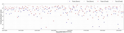
We constructed the data set for ML-model training and test (predict). The S-NPP/VIIRS snow cover product was used as reference data for model training and for evaluating the predicted snow cover. We used S-NPP/VIIRS snow cover product of 2475 scenes during the study period (January–March 2020). To ensure the true value for training, we used 1732 scenes (70% of the total), and we used 743 scenes (30% of the total) as validation data for the integrated snow data applied to the reclassified snow/cloud data by the ML model. Data for training and test (predict) were randomly classified. Figure 4 shows the distribution of training and test data for snow/cloud discrimination during the study period. In addition, this study performed only verification using S-NPP/VIIRS snow cover data from April 2020 to March 2021, including non-winter season, to in-depth analyze the performance of integrated snow cover calculated through ML. From April 2020 to March 2021, the S-NPP/VIIRS snow cover was 2152. Through the corresponding scenes, it is possible to evaluate the accurate separation performance of ML snow and clouds in the off-winter season. Accordingly, we used 1732 scenes for training of ML models, and 2895 scenes were used for validation.

Figure 4. Time series snow and cloud pixel count in the data set for training and test snow/cloud discrimination model (January-March, 2020).

Each data set was applied equally to the RF and DNN models. As the purpose of the study is to improve the part that discriminates snow/cloud in GK-2A/AMI snow cover product, we selected the input data to be applied to our model from among the input data used in the GK-2A/AMI snow cover detection. The data set included two TOA reflectances (R_1.38μm, R_1.61μm), three brightness temperatures (T_3.8μm, T_11.2μm, T_12.3μm) from the GK-2A/AMI channel and index related to channel data (NDSI, Normalized Difference Water Index [NDWI], Brightness Temperature Difference [BTD; T_11.2μm–T_3.8μm]), R anomaly _1.61μm, latitude, SZA, and VZA. R_1.38μm, which belongs to the strong water vapor absorption wavelength band, is used together with R_1.61μm to detect high ice clouds and water clouds (Pavolonis, Heidinger, and Uttal 2005). Because high ice clouds have spectral properties similar to those of snow, it is difficult to distinguish the two. For this reason, we used R_1.38μm to distinguish between ice clouds and snow. R_1.61μm, a representative wavelength band that distinguishes snow from cloud in the SWIR wavelength band, is used in many studies to detect snow or to differentiate between snow and cloud (Huang et al. 2010; Zhu, Wang, and Woodcock 2015). Infrared bands, including T_3.8μm, T_11.2μm, and T_12.3μm, in which the brightness temperature in the cloud region is cooler than the ground surface, are used in cloud detection using threshold-based methods (Rossow and Garder 1993; Saunders and Kriebel 1988). BTD (T_11.2μm–T_3.8μm) is used to detect low-level clouds during daytime or dawn (Le GLeau 2016). NDSI, which is calculated using red and SWIR bands such as Equation (1), is an index used to detect snow cover (Choi and Bindschadler 2004; Hall, Riggs, and Salomonson 1995). NDWI, which is calculated using NIR and SWIR bands such as Equation (2), is sensitive to snow grain size (Eppanapelli et al. 2018). (Imai and Yoshida 2016) used the Himawari-8/AHI cloud detection algorithm to differentiate between snow/ice and cloud. The R anomaly _1.61μm is an index that utilizes the feature that the snow cover has a lower reflectance in the SWIR wavelength band than the visible wavelength band, and Lee et al. (2017) used it to perform snow cover detection. Latitude has been used to identify potential snow cover areas in snow studies (Riggs, Hall, and Román 2016; Romanov 2017). Finally, the spectral properties of snow and cloud depend on various environmental conditions, in particular angle (King et al. 1997; Xin et al. 2012). Therefore, GOES-16/ABI snow cover uses angle (SZA, VZA) data as input data when producing snow cover (Key et al. 2020). The training data consisted of reflectance, brightness temperature, and various indices. Accordingly, the values of the training data variables were quite diverse. Using these values as training data for the ML model would inevitably decrease the performance of the model. We prevented this through a normalization process that limited the values of the training/test data set variables to between 0 and 1 (Equation (3)). The V of Equation (3) is input variable. In this study, the dependent input variable of the model was the snow and cloud pixel of the S-NPP/VIIRS snow cover product. (1) $\mathrm{NDSI}={\displaystyle \frac{R_{0.64\mu \mathrm{m}}-R_{1.61\mu \mathrm{m}}}{R_{0.64\mu \mathrm{m}}+R_{1.61\mu \mathrm{m}}}}$(1) (2) $\mathrm{NDWI}={\displaystyle \frac{R_{0.86\mu \mathrm{m}}-R_{1.61\mu \mathrm{m}}}{R_{0.86\mu \mathrm{m}}+R_{1.61\mu \mathrm{m}}}}$(2) (3) $\mathrm{Normalized}V={\displaystyle \frac{V-V_{min}}{V_{max}+V_{min}}}$(3)

3.2.3. Platform for training models

In this paper, all ML models were performed in Google Colaboratory (Colab) with Python 3.7 based on jupyter notebook. Google Colaboratory (a.k.a Colab) is a project that has the objective of disseminating machine learning education and research (Google 2018). Its user provided with a Tesla T4 GPU device with about 12 GB temporary RAM and 358 GB temporary storage space, which is sufficient to meet the model training requirements in this study (Carneiro et al. 2018). We used TensorFlow and Keras libraries to run ML models in python.

3.2.4. Training models

We empirically adjusted each model’s hyperparameters for RF and DNN model optimization for the purpose of classifying snow and cloud. Two parameters in total were set in the RF model, and we set the N-estimator to 50. Max-depth was set to 25. The DNN model was trained in the order of model structure construction and model learning. Table 1 details the structure of the DNN model and the parameters and their values set during the training process. For model training, learning rate, the maximum number of epochs, batch size, and early stopping patience were set to prevent overfitting. We used the Rectified Linear Unit (ReLU) function for each hidden layer, and the sigmoid function was used because the purpose of the final layer was to determine the presence of snow/cloud. The sigmoid function is suitable for binary classification. We defined the method using the RF model in the snow/cloud discrimination process as Method A and the method using the DNN model as Method B. Method C is a snow/cloud discrimination process that classifies only those pixels for which both RF-based data and DNN-based data are reclassified as snow cover for cloud pixels of GK-2A/AMI snow cover. Lastly, If any one of the two models (RF and DNN) was classified as an snow, the process of classifying the corresponding pixel as snow was defined as Method D.

Table 1. Hyperparameters for the optimal DNN model for snow/cloud discrimination.

Hyperparameter	Value
Hidden layer	4
Node	500
Dropout	0.2
Early stopping (Patience)	20
Learning rate	0.0001
Batch-size	1024
Epoch	400

3.3. Post-processing and accuracy assessment

In order to correctly reclassify the cloud classification area as snow cover pixels in the GK-2A/AMI snow cover, snow was reclassified through four types of ML models (Method A, B, C and D) for pixels classified as clouds in the GK-2A/AMI snow cover. In other words, in order to reclassify the snow cover in the cloud area, we used ML models to discriminate the snow/cloud. Four types of ML-based reclassified snow cover performed simple fusion with pixels not classified as clouds in GK-2A/AMI snow cover. We named the fused data of ML-based integrated snow cover and GK-2A/AMI snow cover as ML-based integrated snow cover. The four types of ML-based integrated snow cover are created; ML-based Method A, B, C and D integrated snow cover. The validation indices used to evaluate the snow/cloud discrimination were precision, recall, overall accuracy (OA), and F1-score. Precision (see Equation (4)), the ratio of pixels classified as snow by validation data to that classified as snow by the model, can be expressed as follows: (4) $\mathrm{Precision}={\displaystyle \frac{\mathrm{TP}}{\mathrm{TP}+\mathrm{FP}}}$(4)

Recall (see Equation (5)), the ratio of pixels classified as snow by the model to the area classified as snow by the validation data, can be expressed as follows: (5) $\mathrm{Recall}={\displaystyle \frac{\mathrm{TP}}{\mathrm{TP}+\mathrm{FN}}}$(5)

OA (see Equation (6)), an evaluation index that intuitively assesses a model’s performance, can be expressed as follows: (6) $\mathrm{OA}={\displaystyle \frac{\mathrm{TP}+\mathrm{TN}}{\mathrm{TP}+\mathrm{TN}+\mathrm{FP}+\mathrm{FN}}}$(6)

The F1-score (see Equation (7)) is the harmonic average of precision and recall. It can accurately evaluate a model’s performance when the data label has an unbalanced structure and can express the performance as a single number. It can be expressed as follows: (7) $\mathrm{F}1\text{-}\mathrm{score}=2\times {\displaystyle \frac{\mathrm{Precision}\times \mathrm{Recall}}{\mathrm{Precision}+\mathrm{Recall}}}$(7)

True positive (TP) in Equations (4)–(7) is the number of pixels classified as snow by both the model and the validation data. False positive (FP) is the number of pixels classified as snow in our model but as cloud by the validation data. False negative (FN) is the number of pixels detected by our model as cloud and by the validation data as snow. True negative (TN) is the number of pixels detected as cloud by both our model and the validation data.

3.4. Evaluation of input variables importance for snow/cloud discrimination

We discriminated snow/cloud by applying 12 input variables to the RF model and DNN model. We trained RF and DNN models optimized for snow/cloud discrimination using 12 input variables. The performance of ML models has a lot of influence on the model type and input variables other than hyperparameters. Therefore, we analyzed how the 12 input variables affected the snow/cloud discrimination accuracy when the trained RF and DNN models were run.

In the evaluation of the importance of input variables in the RF model, there are elements that evaluate the importance of input variables in the RF model. It can measure input variable importance by the average impurity reduction computed across all decision trees in the RF model. The importance of each variable can be evaluated using GINI to evaluate the importance of each variable using the RF model (Menze et al. 2009). In the RF model, GINI is calculated over all trees as the average reduction in node impurities for one segmentation variable (Yao et al. 2022). Since significant variables can substantially reduce the impurities in the sample, the higher the GINI value, the greater the importance of the variable (Simonetti, Simonetti, and Preatoni 2014).

In the case of a DNN model, the DNN model itself does not provide input variable contribution evaluation. To this end, we applied the input variable contribution evaluation method of the DNN model performed by Zamani Joharestani et al. (2019). The performance of the trained DNN model considering all 12 input variables was utilized for accuracy. The performance of the trained model was evaluated by excluding one input variable among 12 input variables. In the case of variables with high importance, the features that reduced the performance of the model were utilized.

4. Results

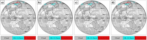
4.1. Snow mapping results of ML-based integrated snow cover

We produced four types of integrated snow cover using RF and DNN models. Figure 5 shows the integrated snow cover through four ML-based methods. The cyan color in Figure 5 is the area classified as snow cover in the GK-2A/AMI snow cover, and the red color is the area where the cloud area is reclassified as snow cover through the ML-based method. It was confirmed that the areas reclassified as snow cover through the snow/cloud discrimination using methods using ML mainly appeared in areas above 50°N. When comparing the snow mapping area of Method A-integrated snow cover (Figure 5a) using RF model and Method B-integrated snow cover (Figure 5b) using DNN model, there were many snow areas where the RF model was reclassified through snow/cloud discrimination. In addition, most of the areas classified as snow covered by Method B-integrated snow cover were also classified as snow covered by Method A-integrated snow cover. This feature is shown in Method C-integrated snow cover. The reclassified snow area of the Method C-integrated snow cover (only pixels reclassified by snow simultaneously in the RF and DNN models; Figure 5c) is similar to the reclassified snow area of the Method B-integrated snow cover. On the other hand, the reclassified snow area of the method D-integrated snow cover (if either the RF model or the DNN model is reclassified by snowfall; Figure 5d) is similar to the reclassified snow area of the method A-integrated snow cover. This can lead to the result that the RF model has better snow/cloud discrimination than the DNN model. However, this section is an analysis of simple snow mapping. In order to estimate the performance of the snow/cloud discrimination of the RF and DNN model, in the next section, we analyzed the results of validation using other satellite-based snow cover and ground observation data.

Figure 5. Snow mapping result through fusion with the GK-2A/AMI snow cover product, 4 March 2020, 04:00 UTC: (a) Method A-integrated snow cover, (b) Method B-integrated snow cover, (c) Method C-integrated snow cover, (d) Method D-integrated snow cover.

4.2. Validation and comparison

We evaluated snow/cloud discrimination on four types of integrated snow cover fused with the GK-2A/AMI snow cover product. To evaluate the extent to which the snow/cloud discrimination of the integrated snow cover reclassified by machine learning (RF and DNN) was improved compared to the traditional method-based snow cover, we also evaluated the GK-2A/AMI snow cover product. In the sections below, we performed not only quantitative validation through assessment of accuracy, but also qualitative validation using other satellite-based snow cover and ground truth data.

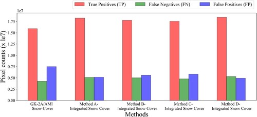
4.2.1. Comparison of ML-based data and other satellite-based data

Figure 6 is the result of comparing the snow/cloud data classified in the GK-2A/AMI snow cover product and the integrated snow cover to the snow/cloud data of the other satellite-based snow cover. The other satellite-based snow cover to be used as validation data in this study was the S-NPP/VIIRS snow cover product. As shown in Figure 6, the integrated snow cover applied using the ML model classified 10.50–6.10% more actual snow than the GK-2A/AMI snow cover product. Among the integrated snow cover, the Method A-integrated snow cover showed 2.5% better snow detection than the Method B-integrated snow cover. The Method D-integrated snow cover that combined the RF and DNN model was affected by the snow detection of the Method A-integrated snow cover, and so it showed the highest number of TP pixels.

Figure 6. The number of true positive, false negative, and false positive snow pixels detected by the GK-2A/AMI snow cover product and the integrated snow cover (January 2020–March 2021); TP (GK-2A/AMI or integrated snow cover – snow and S-NPP/VIIRS snow cover – snow), FN (GK-2A/AMI or integrated snow cover – snow and S-NPP/VIIRS snow cover – cloud), FP (GK-2A/AMI or integrated snow cover – cloud and S-NPP/VIIRS snow cover – snow).

Table 2 presents the results of a quantitative validation using the S-NPP/VIIRS snow cover product for the Method A-, B-, C- and D-integrated snow cover and the GK-2A/AMI snow cover product.

Table 2. Evaluation of snow/cloud discrimination for Method A-, B-, C-, D-integrated snow cover and the GK-2A/AMI snow cover product.

Method	Precision (%)	Recall (%)	F1-score (%)	Overall accuracy (%)
GK-2A/AMI snow cover	67.99	78.95	73.06	89.99
Method A-integrated snow cover	77.97	78.18	78.07	91.26
Method B-integrated snow cover	76.00	78.02	77.00	90.94
Method C-integrated snow cover	75.08	78.56	76.78	90.93
Method D-integrated snow cover	78.89	77.67	78.28	91.26

For the integrated snow cover applied using ML models, the misclassification of snow as cloud was improved compared to the GK-2A/AMI snow cover product. The precision accuracy of the integrated snow cover data was 7.09–10.89% higher than that of the GK-2A/AMI snow cover product (integrated snow cover: 75.08–78.89%, GK-2A/AMI snow cover product: 67.99%). In the recall validation index, the integrated snow cover showed 0.39–1.28% lower accuracy than the GK-2A/AMI snow cover product (integrated snow cover: 77.67–78.56%, GK-2A/AMI snow cover product: 78.95%). We confirmed that the integrated snow cover product had greater precision and OA (GK-2A/AMI snow cover product: 89.99%, integrated snow cover: 90.93–91.26%) than the GK-2A/AMI snow cover product, but the recall accuracy was low. We also confirmed the F1-score, which is the harmonic average of precision and recall. The accuracy of the F1-score of the integrated snow cover was more than 3.71–5.21% higher than that of the GK-2A/AMI snow cover product (integrated snow cover: 76.78–78.28%, GK-2A/AMI snow cover product: 73.06%). Among the integrated snow cover, Method A-integrated snow cover (OA: 91.26%, F1-score: 78.07%) and Method D-integrated snow cover (OA: 91.26%, F1-score: 78.28%) showed excellent snow/cloud discrimination performance.

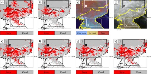
Through qualitative analyses, we also confirmed the spatial characteristics of the integrated snow cover. Figure 7 compares images for the 23 February 2020, 03:40 UTC, scene in the northern Korean Peninsula and adjacent Northeast China (latitude 38.14°N–43.36°N, longitude 123.72°E–130.13°E). Box A in Figure 7 is judged to be a snow area based on analyses of true-color RGB and snow–fog RGB images. The S-NPP/VIIRS snow cover product detected Box A as snow, whereas the GK-2A/AMI snow cover product and Method B- and C-integrated snow cover classified it as cloud. Method A- and D-integrated snow cover reclassified it as snow, the integrated snow cover classified the snow area most similar to the S-NPP/VIIRS snow cover product. Method D-integrated snow cover correctly classified Box A as snow, affecting the snow data reclassified by the RF model. Box B in Figure 7 was classified as cloud based on analyses of true-color RGB and snow–fog RGB images. The S-NPP/VIIRS snow cover product erroneously classified some areas of Box B as snow, whereas the GK-2A/AMI snow cover product and Method A-, B-, C- and D-integrated snow cover classified Box B as cloud.

Figure 7. A comparison of result images: (a) S-NPP/VIIRS snow cover at 03:42 UTC on 23 February 2020, (b) GK-2A/AMI snow cover at 03:40 UTC on 23 February 2020, (c) GK-2A/AMI snow–fog RGB (23 February 2020, 03:40 UTC), (d) GK-2A/AMI true-color RGB (same as GK-2A/AMI scene), (e) Method A-integrated snow cover (same as GK-2A/AMI scene), (f) Method B-integrated snow cover (same as GK-2A/AMI scene), (g) Method C-integrated snow cover (same as GK-2A/AMI scene), (h) Method D-integrated snow cover (same as GK-2A/AMI scene).

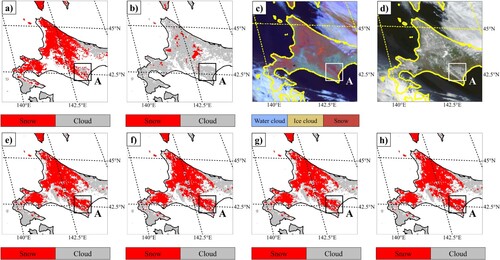
Figure 8 presents comparison and validation results for the 26 March 2020, 03:40 UTC, scene in Hokkaido, Japan (latitude 41.30°N–46.16°N, longitude 138.65°E–145.59°E). The Hokkaido area in Figure 8 was determined as a snow and snow-free land area based on the GK-2A/AMI-based RGB image and the S-NPP/VIIRS snow cover product. However, in the GK-2A/AMI snow cover product, most actual snow areas were classified as cloud. Meanwhile, the integrated snow cover correctly detected snow. Box A in Figure 8 was judged to be a snow area, but the S-NPP/VIIRS snow cover product incorrectly classified it as cloud. The integrated snow cover correctly classified Box A as snow.

Figure 8. A comparison of result images: (a) S-NPP/VIIRS snow cover at 03:42 UTC on 26 March 2020, (b) GK-2A/AMI snow cover at 03:40 UTC on 26 March 2020, (c) GK-2A/AMI snow–fog RGB (26 March 2020, 03:40 UTC), (d) GK-2A/AMI true-color RGB (same as GK-2A/AMI scene), (e) Method A-integrated snow cover (same as GK-2A/AMI scene), (f) Method B-integrated snow cover (same as GK-2A/AMI scene), (g) Method C-integrated snow cover (same as GK-2A/AMI scene), (h) Method D-integrated snow cover (same as GK-2A/AMI scene).

As comparison result show, in the scenes for which we performed a comparative validation, the GK-2A/AMI snow cover product included several areas in which snow was classified as cloud, and the integrated snow cover correctly reclassified the relevant area as snow. Among the RF and DNN model, the snow cover to which the RF model was applied included more than 6% correctly detected snow than the snow cover data to which the DNN model was applied, and their accuracy was slightly higher.

4.2.2. Comparison of ML-based data and in situ snow observation data

In addition to the indirect validation using the S-NPP/VIIRS snow cover product, we validated the snow cover classified by the integrated snow cover using ground truth data – ASOS in situ snow observation data. In the case of validation using directly observed snow depth data, it is crucial that in situ snow observation data stations not explicitly report zero snow depth when there is no snow on the ground (Romanov 2017). Therefore, in situ data can be used to evaluate only snow detection performance; their ability to evaluate erroneous snow detection is limited. In this study, where snow was on the ground, a station for which a daily snowfall of 0 cm or more was recorded was defined as a snow area and used for validation. After excluding clouds from the validation, we obtained 387 snow cover effective pixels using ASOS in situ snow observation data from January to March 2020 and 2021. Table 3 shows the results of validating the snow detection performance of the GK-2A/AMI snow cover product and integrated snow cover. The integrated snow cover showed higher precision accuracy than the GK-2A/AMI snow cover. Based on only the area providing ASOS in situ snow observation data, the integrated snow cover detected the snow cover 25.38–45.17% more than the GK-2A/AMI snow cover. Among the Method A- and B-integrated snow covers that used the RF model and the DNN model only, the Method A-integrated snow cover that distinguishes snow/clouds using the RF model alone had excellent snow detection performance. Method C-integrated snow cover showed similar snow detection performance to Method B-integrated snow cover, which performed snow/cloud discrimination using the DNN model only. This means that, considering the characteristics of Method C, most of the pixels in the snow reclassified by the DNN model were also reclassified as snow covered by the RF model. Method D-integrated snow cover showed similar snow detection performance to Method A-integrated snow cover, which performed snow/cloud discrimination using RF model alone. In addition, Lee and Choi (2022) used the high temporal resolution characteristics of geostationary meteorological satellites to distinguish snow cover from clouds, and performed daily snow cover mapping using GK-2A/AMI data. As a result of comparison with ASOS in-situ data, which is one of the snow mapping results, the precision was 70.32%, which was similar to our result during 2 months (1 Dec. 2020 to 31 Jan. 2021). Our study was performed on 10-minute snow cover, and the method proposed by Lee and Choi (2022) was targeted for daily snow cover.

Table 3. Evaluation results of snow cover detection for GK-2A/AMI snow cover product, Method A-, B-, C-, D-integrated snow cover and Lee and Choi (2022) result using ASOS in situ snow observation data; TP: True Positives, FP: False Positives.

Method	TP	FP	Precision (%)	Temporal scale
GK-2A/AMI snow cover	197	190	50.90	10-minutes
Method-A integrated snow cover	285	102	73.64	10-minutes
Method-B integrated snow cover	248	139	64.08	10-minutes
Method-C integrated snow cover	247	140	63.82	10-minutes
Method-D integrated snow cover	286	101	73.90	10-minutes
Lee and Choi (2022)	–	–	70.32	1-day

4.3. Evaluation of input variable importance for snow/cloud discrimination

4.3.1. Random forest

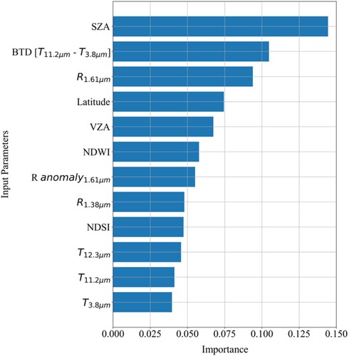
Figure 9 is the result of quantitatively showing the contribution of snow/cloud discrimination to the 12 input variables when applying the trained RF model for snow/cloud discrimination to the 12 input variables. The variable with the greatest effect on snow/cloud discrimination was SZA. SZA has a considerable influence on the spectral properties of snow and cloud (King et al. 1997; Li, Li, and Xiao 2016) and thus significantly influences snow/cloud discrimination. In addition, BTD (T_11.2μm–T_3.8μm) and NDWI are used in the cloud detection algorithm of the same geostationary meteorological satellite Himawari-8/AHI to distinguish cloud area from snow/ice (Le GLeau 2016). Accordingly, in this study, which classified snow/cloud using RF model, it was judged as having a strong influence. R_1.61μm is an SWIR wavelength band that is widely used to distinguish snow and cloud using the threshold method (Huang et al. 2010; Zhu, Wang, and Woodcock 2015). This variable also had a significant influence on the classification of snow and cloud using the RF model. The NDSI, a representative index used for snow detection, showed low sensitivity to snow/cloud discrimination. NDSI shows a value distribution of 0.4 or more in the snow-covered area, but as VZA is higher, the NDSI value in the snow-covered area tends to decrease (Xin et al. 2012). Although this study set the FD area of geostationary meteorological satellites as the study area, most of the actual areas where snow/cloud discrimination was performed had VZA of 40° or more. Accordingly, the sensitivity of NDSI to snow/cloud discrimination was judged to have decreased.

Figure 9. Importance of input variables used in RF model for snow/cloud discrimination.

4.3.2. Deep neural network model

Table 4 shows the effect of feature permutation on the performance of the trained DNN model for snow/cloud discrimination. It shows the snow/cloud discrimination accuracy of the trained DNN model with all 12 input variables applied and the trained DNN model excluding one of the 12 input variables. Snow/cloud discrimination accuracy (overall accuracy, OA) used the validation accuracy of the model when training the model. We derived model validation accuracy by repeating DNN training 13 times, considering the 12 input variables applied to the DNN model. The accuracy that shows the best DNN model performance through these procedures is 0.8732, and this accuracy is when all 12 input variables are used. We evaluated the importance ranking of each variable as shown in Table 4 based on the validation accuracy of the snow/cloud discrimination model for 12 cases excluding one of the 12 input variables. Ranking in Table 4 was organized using the validation accuracy of 12 cases. Among the 12 variables, the variable showing the highest importance in the discrimination of snow/cloud is shown as SZA in the same way as in the RF model. In addition, among the 12 input variables, the top 5 of the importance of snow/cloud discrimination in the RF and DNN models were composed of the same variables; SZA, VZA, BTD (T_11.2μm–T_3.8μm), R_1.61μm and latitude. In addition to geometry parameters such as SZA, VZA, and latitude, physical variables include BTD (T_11.2μm–T_3.8μm) and R_1.61μm. These are representative variables used to discriminate snow/clouds as discussed in the evaluation of the importance of input variables in the RF model. In the NDSI, the importance of snow/cloud discrimination was low in the DNN model as in the RF model.

Table 4. Features permutation of a trained deep neural network (DNN) model and features permutation effect on the snow/cloud discrimination performance.

Permuted feature	Overall accuracy	Ranking
SZA	0.8417	1
VZA	0.8614	2
Latitude	0.8617	3
BTD (T11.2μm–T3.8μm)	0.8649	4
R1.61μm	0.8663	5
R anomaly 1.61μm	0.8666	6
NDSI	0.8669	7
T12.3μm	0.8676	8
R1.38μm	0.8681	9
NDWI	0.8682	10
T11.2μm	0.8687	11
T3.8μm	0.8689	12
Trained DNN model (12 input variables)	0.8732	–

5. Discussions

5.1. ML models for snow/cloud discrimination

To improve the snow/cloud discrimination performance of GK-2A/AMI snow cover, we evaluated whether it is suitable for snow/cloud discrimination using RF and DNN models. It was confirmed that the snow cover reclassified through the snow/cloud discrimination using the RF model classified the actual snow cover more than the snow cover reclassified through the snow/cloud discrimination using the DNN model. Method C-integrated snow cover, which is reclassified as snow when both models are classified as snow in the RF and DNN models, showed similar snow mapping to Method B-integrated snow cover using only the DNN model only. In addition, Method D-integrated snow cover, which reclassifies as snow when even one of the RF and DNN models is classified as snow through snow/cloud discrimination, was similar to the method A-integrated snow cover and snow mapping results using only RF models. This means that most of the areas reclassified by the DNN model as snow cover were also reclassified by the RF model as snow cover. The RF model shows similar results to other studies showing better results for classification (Baek and Jung 2021).

5.2. Application of ML models to operational satellite-based snow cover

Many remote sensing studies have used ML model and validated their utility (Belgiu and Drăgut 2016; Varshney et al. 2018; Xia et al. 2019). ML models are applied to satellite-based data provided by an advanced institution rather than during the research stage. In the satellite-based snow cover data, we performed snow/cloud discrimination, which is a key contributing factor of uncertainty, through ML model, and fused to operational satellite-based snow cover through post-processing. To apply ML models to operational satellite-based snow cover data, we considered the variables used in the GK-2A/AMI snow cover detection algorithm when selecting the input variables for our ML models. The ML-based integrated snow cover fused with the GK-2A/AMI snow cover product showed improved snow/cloud discrimination compared to the GK-2A/AMI snow cover product. The results in this study indicate that it is possible to apply ML methods with excellent snow/cloud discrimination to traditional method-based snow cover. In particular, we demonstrated the results of applying ML-based snow/cloud discrimination data to operational geostationary satellite-based snow cover as a post-processing process. We tested the snow/cloud discrimination performance of the ML model from January 2020 to March 2021. Through the evaluation of the snow/cloud discrimination performance of the ML model for more than one year, it was confirmed that the RF model had better snow/cloud discrimination performance than the DNN model. However, although data were collected for more than one year, there were insufficient samples to measure the snow/cloud discrimination performance in Australia and New Zealand, which belong to the southern hemisphere, among the GK-2A/AMI observation. In addition, the ground truth data was validated by acquiring only the South Korea data. In future studies, we will collect enough samples to evaluate the snow/cloud discrimination performance of the southern hemisphere region included in the GK-2A/AMI observation region, and collect ground truth data outside South Korea to conduct ML model tests for snow/cloud discrimination. Also, in future research, we plan to conduct not only the snow/cloud discrimination performance of the ML model, but also how the ML model affects the snow cover/cloud classification and whether there are regional variations.

6. Conclusion

We focused on the misclassification of actual snow cover as clouds among potential error factors in the snow/cloud discrimination of operational satellite-based snow cover. To improve this part, two ML models (RF and DNN) were applied to evaluate which ML model is suitable for snow/cloud discrimination. The satellite-based snow cover data is the GK-2A/AMI snow cover product, and the snow/cloud discrimination error of the GK-2A/AMI snow cover product was confirmed. We reclassified the snow cover by applying ML to the pixels classified by clouds in the GK-2A/AMI snow cover product. As a result of applying ML for snow/cloud discrimination, it was confirmed that ML improved the potential error factors of satellite-based snow cover. Among the RF and DNN model, it was also found that the RF model was suitable for snow/cloud discrimination. Through this study, we confirmed the possibility of improving the limitations of the traditional method-based snow/cloud discrimination data through post-processing using a ML model. In that this is not a presentation of a ML model that replaces the traditional snow/cloud discrimination methods, it can confirm the difference from other studies for snow/cloud discrimination. Our study results show that the ML model for snow/cloud discrimination can be applied not only to satellite-based snow data, but also to cloud detection algorithms. In addition, it is significant that not only a single ML model but also two multiple ML models were applied to snow/cloud discrimination. The ML model application process presented by us can also be applied to traditional method-based snow cover through post-processing. If this is used, it is judged that the accuracy of satellite-based snow cover will be improved in the future. In the future, when developing a snow cover detection algorithm including snow/cloud discrimination based on the results of this study, a method that combines the advantages of traditional method and ML model can be considered. In addition, this study evaluated the importance of input variables used for snow/cloud discrimination. Input variable importance evaluation was performed on both the trained RF and DNN models. The results of evaluating the importance of input variables used to classify snow/clouds can help in future snow/cloud discrimination studies. In particular, when applied to geostationary satellites, the observation period is 10 min and high-quality snow cover data with high temporal resolution can be produced. High-quality snow cover data has high utility in elucidating the relationship between climate change, especially global warming. In addition, it can be used to investigate the relationship between snow cover and healthy, energy utilization and vegetation growth. In addition, high-quality snow detection data can be used as input data for other meteorological products to which snow detection data is used as input data.

Acknowledgements

The authors would like to thank the National Meteorological Satellite Center (NMSC) of the Korea Meteorological Administration (KMA), South Korea for their support in carrying out this work. We’d like to appreciate the editors and anonymous reviewers, whose comments are all valuable and very helpful for improving our manuscript. The GK-2A images used in this study are distributed in NMSC at https://nmsc.kma.go.kr/enhome/html/main/main.do. The ASOS in situ snow observation data used in this study are distributed in KMA at https://data.kma.go.kr/data/grnd/selectAsosRltmList.do?pgmNo=36. The S-NPP/VIIRS data used in this study are distributed in NASA at https://search.earthdata.nasa.gov/search. We would like to greatly appreciate the reviewers and the editors for their valuable comments.

Disclosure statement

No potential conflict of interest was reported by the author(s).

Data availability statement

The data that support the findings of this study are openly available in ‘figshare’ at https://doi.org/10.6084/m9.figshare.20488971.v2.

Additional information

Funding

This work was supported by the National Research Foundation of Korea (NRF) grant funded by the Korean government (MSIT) [grant number 2021R1A2C2010976].

References

- Baek, Won-Kyung, and Hyung-Sup Jung. 2021. “Performance Comparison of oil Spill and Ship Classification from X-Band Dual-and Single-Polarized sar Image Using Support Vector Machine, Random Forest, and Deep Neural Network.” Remote Sensing 13 (16): 3203.
- Bair, Edward H., Robert E. Davis, and Jeff Dozier. 2018. “Hourly Mass and Snow Energy Balance Measurements from Mammoth Mountain, CA USA, 2011–2017.” Earth System Science Data 10 (1): 549–563.
- Belgiu, Mariana, and Lucian Drăgut. 2016. “Random Forest in Remote Sensing: A Review of Applications and Future Directions.” ISPRS Journal of Photogrammetry and Remote Sensing 114: 24–31.
- Biemans, H., C. Siderius, A. F. Lutz, S. Nepal, B. Ahmad, T. Hassan, Werner von Bloh, et al. 2019. “Importance of Snow and Glacier Meltwater for Agriculture on the Indo-Gangetic Plain.” Nature Sustainability 2 (7): 594–601.
- Bui, Dieu Tien, Nhat-Duc Hoang, Francisco Martínez-Álvarez, Phuong-Thao Thi Ngo, Pham Viet Hoa, Tien Dat Pham, Pijush Samui, and Romulus Costache. 2020. “A Novel Deep Learning Neural Network Approach for Predicting Flash Flood Susceptibility: A Case Study at a High Frequency Tropical Storm Area.” Science of the Total Environment 701: 134413.
- Cannistra, Anthony F., David E. Shean, and Nicoleta C. Cristea. 2021. “High-Resolution CubeSat Imagery and Machine Learning for Detailed Snow-Covered Area.” Remote Sensing of Environ- Ment 258: 112399.
- Carneiro, Tiago, Raul Victor Medeiros Da Nóbrega, Thiago Nepomuceno, Gui-Bin Bian, Victor Hugo C. De Albuquerque, and Pedro Pedrosa Reboucas Filho. 2018. “Performance Analysis of Google Colaboratory as a Tool for Accelerating Deep Learning Applications.” IEEE Access 6: 61677–61685.
- Chaujar, Ravinder Kumar. 2009. “Climate Change and Its Impact on the Himalayan Glaciers–a Case Study on the Chorabari Glacier, Garhwal Himalaya, India.” Current Science, 96, 703–708.
- Choi, Hyeungu, and Robert Bindschadler. 2004. “Cloud Detection in Landsat Imagery of Ice Sheets Using Shadow Matching Technique and Automatic Normalized Difference Snow Index Threshold Value Decision.” Remote Sensing of Environment 91 (2): 237–242.
- Choi, Sungwon, Donghyun Jin, Noh-Hun Seong, Daeseong Jung, Suyoung Sim, Jongho Woo, Uujin Jeon, Yugyeong Byeon, and Kyung-soo Han. 2021. “Near-Surface Air Temperature Retrieval Using a Deep Neural Network from Satellite Observations Over South Korea.” Remote Sensing 13 (21): 4334.
- Cilli, Roberto, Alfonso Monaco, Nicola Amoroso, Andrea Tateo, Sabina Tangaro, and Roberto Bellotti. 2020. “Machine Learning for Cloud Detection of Globally Distributed Sentinel-2 Images.” Remote Sensing 12 (15): 2355.
- Cohen, Judah, and David Rind. 1991. “The Effect of Snow Cover on the Climate.” Journal of Climate 4 (7): 689–706.
- Croce, Pietro, Paolo Formichi, Filippo Landi, Paola Mercogliano, Edoardo Bucchignani, Alessandro Dosio, and Silvia Dimova. 2018. “The Snow Load in Europe and the Climate Change.” Climate Risk Management 20: 138–154.
- De Gregorio, Ludovica, Mattia Callegari, Carlo Marin, Marc Zebisch, Lorenzo Bruzzone, Begüm Demir, Ulrich Strasser, et al. 2019. “A Novel Data Fusion Technique for Snow Cover Retrieval.” IEEE Journal of Selected Topics in Applied Earth Observations and Remote Sensing 12 (8): 2862–2877.
- Domine, Florent, Mathieu Barrere, Denis Sarrazin, Samuel Morin, and Laurent Arnaud. 2015. “Automatic Monitoring of the Effective Thermal Conductivity of Snow in a low-Arctic Shrub Tundra.” The Cryosphere 9 (3): 1265–1276.
- Dozier, Jeff. 1989. “Spectral Signature of Alpine Snow Cover from the Landsat Thematic Mapper.” Remote Sensing of Environment 28: 9–22.
- Eppanapelli, Lavan Kumar, Nina Lintzén, Johan Casselgren, and Johan Wåhlin. 2018. “Estimation of Liquid Water Content of Snow Surface by Spectral Reflectance.” Journal of Cold Regions Engineering 32 (1): 05018001.
- Google. 2018. “Colaboratory: Frequently Asked Questions.”
- Groisman, Pavel Ya, Thomas R. Karl, and Richard W. Knight. 1994. “Observed Impact of Snow Cover on the Heat Balance and the Rise of Continental Spring Temperatures.” Science 263 (5144): 198–200.
- Hall, Dorothy K., George A. Riggs, and Vincent V. Salomonson. 1995. “Development of Methods for Mapping Global Snow Cover Using Moderate Resolution Imaging Spectroradiometer Data.” Remote Sensing of Environment 54 (2): 127–140.
- Hall, Dorothy K., and Vincent V. Salomonson. 2006. “MODIS Snow Products User Guide to Collection 5 George A. Riggs.”
- Han, Kyung-Soo, Donghyun Jin, and Kyeong-Sang Lee. 2019. “GK-2A AMI Algorithm Theoretical Basis Document; Snow Cover/Sea-ice Cover.”
- Hao, Xiaohua, Siqiong Luo, Tao Che, Jian Wang, Hongyi Li, Liyun Dai, Xiaodong Huang, and Qisheng Feng. 2019. “Accuracy Assessment of Four Cloud-Free Snow Cover Products Over the Qinghai-Tibetan Plateau.” International Journal of Digital Earth 12 (4): 375–393.
- Härer, Stefan, Matthias Bernhardt, Matthias Siebers, and Karsten Schulz. 2018. “On the Need for a Time-and Location-Dependent Estimation of the NDSI Threshold Value for Reducing Existing Uncertainties in Snow Cover Maps at Different Scales.” The Cryosphere 12 (5): 1629–1642.
- Haynes, J. M., Yoo-Jeong Noh, S. D. Miller, A. Heidinger, and J. M. Forsythe. 2019. “Cloud Geometric Thickness and Improved Cloud Boundary Detection with the GOES ABI.” In 99th American Meteorological Society Annual Meeting, AMS.
- Ho, Tin Kam. 1998. “The Random Subspace Method for Constructing Decision Forests.” IEEE Transactions on Pattern Analysis and Machine Intelligence 20 (8): 832–844.
- Huang, Chengquan, Nancy Thomas, Samuel N. Goward, Jeffrey G. Masek, Zhiliang Zhu, John R. G. Townshend, and James E. Vogelmann. 2010. “Automated Masking of Cloud and Cloud Shadow for Forest Change Analysis Using Landsat Images.” International Journal of Remote Sensing 31 (20): 5449–5464.
- Imai, Takahito, and Ryo Yoshida. 2016. “Algorithm Theoretical Basis for Himawari-8 Cloud Mask Product.” Meteorol. Satell. Center Tech. Note 61: 1–17.
- Key, Jeffrey R., Yinghui Liu, Xuanji Wang, Aaron Letterly, and Thomas H. Painter. 2020. “Chapter 14 - Snow and Ice Products from ABI on the GOES-R series.” In The GOES-R series: A new generation of geostationary environmental satellites, edited by Steven J. Goodman, Timothy J. Schmit, Jaime Daniels, and Robert J. Redmon, 165–177. Elsevier.
- Key, Jeffrey R., Robert Mahoney, Yinghui Liu, Peter Romanov, Mark Tschudi, Igor Appel, James Maslanik, Dan Baldwin, Xuanji Wang, and Paul Meade. 2013. “Snow and ice Products from Suomi NPP VIIRS.” Journal of Geophysical Research: Atmospheres 118 (23): 12–816.
- King, Michael D., Si-Chee Tsay, Steven E Platnick, Menghua Wang, and Kuo-Nan Liou. 1997. “Cloud Retrieval Algorithms for MODIS: Optical Thickness, Effective Particle Radius, and Thermodynamic Phase.” MODIS Algorithm Theoretical Basis Document No. ATBD-MOD-05 MOD06 - Cloud Product: 1–83.
- Latinne, Patrice, Olivier Debeir, and Christine Decaestecker. 2001. “Limiting the Number of Trees in Random Forests.” In Multiple Classifier Systems, edited by Kittler Josef and Roli Fabio, 178–187. Berlin, Heidelberg: Springer.
- Lee, Soobong, and Jaewan Choi. 2022. “A Snow Cover Mapping Algorithm Based on a Multi-Temporal Dataset for GK-2A Imagery.” GIScience & Remote Sensing 59 (1): 1078–1102.
- Lee, Kyeong-Sang, Donghyun Jin, Jong-Min Yeom, Minji Seo, Sungwon Choi, Jae-Jin Kim, and Kyung-Soo Han. 2017. “New Approach for Snow Cover Detection Through Spectral Pattern Recognition with MODIS Data.” Journal of Sensors vol. 2017: 1–15.
- Le GLeau, Herve. 2016. “Algorithm Theoretical Basis Document for the Cloud Product Processors of the NWC/GEO.” Technical Report. Meteo-France, Centre de Meteorologie Spatiale.
- Li, Haixing, Xingong Li, and Pengfeng Xiao. 2016. “Impact of Sensor Zenith Angle on MOD10A1 Data Reliability and Modification of Snow Cover Data for the Tarim River Basin.” Remote Sensing 8 (9): 750.
- Liu, Changyu, Xiaodong Huang, Xubing Li, and Tiangang Liang. 2020. “MODIS Fractional Snow Cover Mapping Using Machine Learning Technology in a Mountainous Area.” Remote Sensing 12 (6): 962.
- Luo, Jianfeng, Chunyu Dong, Kairong Lin, Xiaohong Chen, Liqiang Zhao, and Lucas Menzel. 2022. “Mapping Snow Cover in Forests Using Optical Remote Sensing, Machine Learning and Time-Lapse Photography.” Remote Sensing of Environment 275: 113017.
- Ma, Lei, Yu Liu, Xueliang Zhang, Yuanxin Ye, Gaofei Yin, and Brian Alan Johnson. 2019. “Deep Learning in Remote Sensing Applications: A Meta-Analysis and Review.” ISPRS Journal of Photogrammetry and Remote Sensing 152: 166–177.
- Menze, Bjoern H., B. Michael Kelm, Ralf Masuch, Uwe Himmelreich, Peter Bachert, Wolfgang Petrich, and Fred A. Hamprecht. 2009. “A Comparison of Random Forest and Its Gini Importance with Standard Chemometric Methods for the Feature Selection and Classification of Spectral Data.” BMC Bioinformatics 10 (1): 1–16.
- Miller, Jeffrey, Udaysankar Nair, Rahul Ramachandran, and Manil Maskey. 2018. “Detection of Transverse Cirrus Bands in Satellite Imagery Using Deep Learning.” Computers & Geosciences 118: 79–85.
- Muhuri, Arnab, Simon Gascoin, Lucas Menzel, Tihomir S Kostadinov, Adrian A Harpold, Alba Sanmiguel-Vallelado, and Juan I. López-Moreno. 2021. “Performance Assessment of Optical Satellite-Based Operational Snow Cover Monitoring Algorithms in Forested Landscapes.” IEEE Journal of Selected Topics in Applied Earth Observations and Remote Sensing 14: 7159–7178.
- Musselman, Keith N., Martyn P. Clark, Changhai Liu, Kyoko Ikeda, and Roy Rasmussen. 2017. “Slower Snowmelt in a Warmer World.” Nature Climate Change 7 (3): 214–219.
- Pavolonis, Michael J., Andrew K. Heidinger, and Taneil Uttal. 2005. “Daytime Global Cloud Typing from AVHRR and VIIRS: Algorithm Description, Validation, and Comparisons.” Journal of Applied Meteorology 44 (6): 804–826.
- Platnick, Steven, Michael D. King, Steven A. Ackerman, W. Paul Menzel, Bryan A. Baum, Jérôme C. Riédi, and Richard A. Frey. 2003. “The MODIS Cloud Products: Algorithms and Examples from Terra.” IEEE Transactions on Geoscience and Remote Sensing 41 (2): 459–473.
- Qiao, Dejing, and Nianqin Wang. 2019. “Relationship Between Winter Snow Cover Dynamics, Climate and Spring Grassland Vegetation Phenology in Inner Mongolia, China.” ISPRS International Journal of Geo-Information 8 (1): 42.
- Riggs, George A., and Dorothy K. Hall. 2004. “Snow and Cloud Discrimination Factors in the MODIS Snow Algorithm.” In Proceedings of IGARSS 2004, 2004 IEEE International Geoscience and Remote Sensing Symposium, Anchorage, AK, USA, 20-24 September 2004, Vol. 6, 3714–3716. Piscataway, NJ: IEEE.
- Riggs, G. A., D. K. Hall, and M. O. Román. 2015. “VIIRS Snow Cover Algorithm Theoretical Basis Document (ATBD).” NASA VIIRS Project Document. Greenbelt, MD: NASA Goddard Space Flight Center.
- Riggs, George A., Dorothy K. Hall, and Miguel O. Román. 2016. “NASA S-NPP VIIRS Snow Products Collection 1 User Guide.”
- Rodriguez-Galiano, Victor F., and Mario Chica-Rivas. 2014. “Evaluation of Different Machine Learning Methods for Land Cover Mapping of a Mediterranean Area Using Multi-Seasonal Landsat Images and Digital Terrain Models.” International Journal of Digital Earth 7 (6): 492–509.
- Romanov, Peter. 2017. “Global Multisensor Automated Satellite-Based Snow and ice Mapping System (GMASI) for Cryosphere Monitoring.” Remote Sensing of Environment 196: 42–55.
- Rossow, William B., and Leonid C. Garder. 1993. “Cloud Detection Using Satellite Measurements of Infrared and Visible Radiances for ISCCP.” Journal of Climate 6 (12): 2341–2369.
- Saunders, R. Wl, and K. Ts Kriebel. 1988. “An Improved Method for Detecting Clear sky and Cloudy Radiances from AVHRR Data.” International Journal of Remote Sensing 9 (1): 123–150.
- Scornet, Erwan. 2017. “Tuning Parameters in Random Forests.” ESAIM: Proceedings and Surveys 60: 144–162.
- Siljamo, Niilo, and Otto Hyvärinen. 2011. “New Geostationary Satellite–Based Snow-Cover Algorithm.” Journal of Applied Meteorology and Climatology 50 (6): 1275–1290.
- Simonetti, Edoardo, Dario Simonetti, and Damiano Preatoni. 2014. Phenology-Based Land Cover Classification Using Landsat 8 Time Series. Ispra, Italy: European Commission Joint Research Center.
- Thompson, Lonnie G., Yao Tandong, Mary E. Davis, Ellen Mosley-Thompson, Tracy A. Mashiotta, Ping-Nan Lin, Vladimir N. Mikhalenko, and Victor S. Zagorodnov. 2006. “Holocene Climate Variability Archived in the Puruogangri ice cap on the Central Tibetan Plateau.” Annals of Glaciology 43: 61–69.
- Varshney, D., P. K. Gupta, C. Persello, and B. R. Nikam. 2018. “Snow and Cloud Discrimination Using Convolutional Neural Networks.” ISPRS Annals of the Photogrammetry, Remote Sensing and Spatial Information Sciences 4: 59–63.
- Wang, Chenxi, Steven Platnick, Kerry Meyer, Zhibo Zhang, and Yaping Zhou. 2020. “A Machine-Learning-Based Cloud Detection and Thermodynamic-Phase Classification Algorithm Using Passive Spectral Observations.” Atmospheric Measurement Techniques 13 (5): 2257–2277.
- Wang, Xian, Lei Zhong, and Yaoming Ma. 2022. “Estimation of 30 m Land Surface Temperatures Over the Entire Tibetan Plateau Based on Landsat-7 ETM+ Data and Machine Learning Methods.” International Journal of Digital Earth 15 (1): 1038–1055.
- Warren, Stephen G. 1982. “Optical Properties of Snow.” Reviews of Geophysics 20 (1): 67–89.
- Xia, Min, Wan’an Liu, Bicheng Shi, Liguo Weng, and Jia Liu. 2019. “Cloud/Snow Recognition for Multispectral Satellite Imagery Based on a Multidimensional Deep Residual Network.” International Journal of Remote Sensing 40 (1): 156–170.
- Xie, Yu, Ping Yang, Bo-Cai Gao, George W Kattawar, and Michael I Mishchenko. 2006. “Effect of Ice Crystal Shape and Effective Size on Snow Bidirectional Reflectance.” Journal of Quantitative Spectroscopy and Radiative Transfer 100 (1–3): 457–469.
- Xin, Qinchuan, Curtis E Woodcock, Jicheng Liu, Bin Tan, Rae A Melloh, and Robert E Davis. 2012. “View Angle Effects on MODIS Snow Mapping in Forests.” Remote Sensing of Environment 118: 50–59.
- Yang, Hong, Hengliang Guo, Wenhao Dai, Bingkang Nie, Baojin Qiao, and Liping Zhu. 2022. “Bathymetric Mapping and Estimation of Water Storage in a Shallow Lake Using a Remote Sensing Inversion Method Based on Machine Learning.” International Journal of Digital Earth 15 (1): 789–812.
- Yang, Jianwei, Lingmei Jiang, Kari Luojus, Jinmei Pan, Juha Lemmetyinen, Matias Takala, and Shengli Wu. 2020. “Snow Depth Estimation and Historical Data Reconstruction Over China Based on a Random Forest Machine Learning Approach.” The Cryosphere 14 (6): 1763–1778.
- Yao, Jinxi, Ji Wu, Chengzhi Xiao, Zhi Zhang, and Jianzhong Li. 2022. “The Classification Method Study of Crops Remote Sensing with Deep Learning, Machine Learning, and Google Earth Engine.” Remote Sensing 14 (12): 2758.
- You, Qinglong, Tao Wu, Liuchen Shen, Nick Pepin, Ling Zhang, Zhihong Jiang, Zhiwei Wu, Shushing Kang, and Amir AghaKouchak. 2020. “Review of Snow Cover Variation Over the Tibetan Plateau and Its Influence on the Broad Climate System.” Earth-Science Reviews 201: 103043.
- Zamani Joharestani, M., C. Cao, X. Ni, B. Bashir, and S. Talebiesfandarani. 2019. “PM2.5 Prediction Based on Random Forest, XGBoost, and Deep Learning Using Multisource Remote Sensing Data.” Atmosphere 10 (7): 373.
- Zhan, Yongjie, Jian Wang, Jianping Shi, Guangliang Cheng, Lele Yao, and Weidong Sun. 2017. “Distinguishing Cloud and Snow in Satellite Images via Deep Convolutional Network.” IEEE Geoscience and Remote Sensing Letters 14 (10): 1785–1789.
- Zhang, Yinsheng, and Ning Ma. 2018. “Spatiotemporal Variability of Snow Cover and Snow Water Equivalent in the Last Three Decades Over Eurasia.” Journal of Hydrology 559: 238–251.
- Zhu, Zhe, Shixiong Wang, and Curtis E Woodcock. 2015. “Improvement and Expansion of the Fmask Algorithm: Cloud, Cloud Shadow, and Snow Detection for Landsats 4–7, 8, and Sentinel 2 Images.” Remote Sensing of Environment 159: 269–277.
- Zhu, Zhe, and Curtis E Woodcock. 2012. “Object-Based Cloud and Cloud Shadow Detection in Landsat Imagery.” Remote Sensing of Environment 118: 83–94.
- Zhu, Zhe, and Curtis E Woodcock. 2014. “Automated Cloud, Cloud Shadow, and Snow Detection in Multitemporal Landsat Data: An Algorithm Designed Specifically for Monitoring Land Cover Change.” Remote Sensing of Environment 152: 217–234.