A hybrid model for high spatial and temporal resolution population distribution prediction

ABSTRACT

The accurate prediction of population distribution is crucial for numerous applications, from urban planning to epidemiological modelling. Using one-week data collected from open and multiple sources, including telecommunication activity, weather, point of interest, buildings, roads, and land use in Milan, Italy, we develop a hybrid method combining cellular automata (CA) and long short-term memory (LSTM) to predict population distribution with fine temporal and spatial granularity. Specifically, the convolutional autoencoder and LightGBM are applied to identify missing building types based on the pedestrian shed. The LSTM learns the transition rules of CA and Shapley additive explanations value is used for variable importance analysis. Results demonstrate that the combination of convolutional autoencoder and LightGBM is effective in building type prediction. The proposed model for population distribution prediction outperforms LSTM, the combination of CA and neural network, and the combination of CA and LightGBM by at least 5–10%. A variable importance analysis reveals that temporal variables are the most significant for prediction, followed by spatial and natural variables. The order of hour, housing-related variables, and types of precipitation are the most important variables in each category.

KEYWORDS:

• Cellular automata
• long short-term memory
• spatial and temporal analysis
• big data
• population distribution

1. Introduction

From 2010 to 2020, the world population increased from 7 to 7.8 billion (Gu, Andreev, and Dupre 2021). During this process, advancements in traffic systems have led to increased human mobility, which is a threat to resources. Urban infrastructure development, such as urban planning and demand response, typically requires an accurate estimation of population distribution information at a fine-scale (Lu et al. 2010). For example, information and communications technology (ICT) infrastructure has evolved rapidly in the recent decade to provide a more diversified and customised service to people in urban and rural areas. Furthermore, numerous applications, including network diversity and economic development (Eagle, Macy, and Claxton 2010), micro-scoped urban structure analysis (Louail et al. 2014), land use organisation modelling (Lenormand et al. 2015), and prompt public health policy-making, require high-resolution population distribution data. Therefore, a fine-scale estimation of population distribution is needed. Technically, predicting population distribution in small spatial and temporal granularity is challenging.

The advance in communication and positioning technologies makes it possible to generate massive mobile signalling data. There are 128 mobile cellular subscriptions per 100 people in Italy, which makes mobile signalling most representative for high spatial and temporal population distribution. Mobile signalling data has been used to study people’s mobility pattern at a large spatial scale (González, Hidalgo, and Barabási 2008; Alessandretti, Aslak, and Lehmann 2020). In addition, several population data products have been developed based on mobile signalling data. Such as WorldPop developed by the University of Southampton, UK.

Another challenge is that the distribution of people is affected by various factors, such as building distribution (Zhao et al. 2020), roads (Cooper et al. 2018), weather conditions (Huang et al. 2015), and time (Eon et al. 2018). These factors can be divided into spatial and temporal factors. However, most studies have comprehensively focused on the influence of buildings, roads, time, and weather; the comprehensive analysis of each variable's contribution to prediction performance has not been thoroughly discussed.

Model-based methods are widely used to solve natural evolution problem and show satisfactory performance. However, acquiring the simulation rules of these models is difficult. Because of the development of computational intelligence, data-driven methods have been widely used to capture nonlinear relations using real-world data (Bzdok, Altman, and Krzywinski 2018).

The aim of this study is to take advantage of both model-based method and machine learning method to improve prediction performance and quantify the contribution of each influencing factors. The contribution can be summarised as follows:

1. A framework combing CA and LSTM was developed to improve the prediction performance of population distribution in high spatial and temporal resolution.

2. Geometry and spatial characteristics of buildings was firstly considered to predict building type.

3. The contribution of various influencing factors on population distribution prediction was quantified.

The remainder of this paper is organised as follows. Section 2 reviews research on the population distribution prediction and the evaluation of related factors. Section 3 describes the study framework, data collection and pre-processing, and the proposed method. Section 4 provides the data analysis results, building type prediction, population distribution prediction, and variable importance analysis. Finally, the conclusions and directions for future work are presented in Section 5.

2. Literature review

This section discusses the factors influencing population distribution and compares state-of-the-art techniques for population distribution prediction, which are classified into two groups: model-based or data-driven methods. Then the current practices and challenges of hybrid prediction techniques are further discussed.

2.1. Influencing factors of population distribution

Population distribution is highly dynamic and challenging to predict because of the complex nature of people’s movement (Vu, Do, and Nahrstedt 2011). The literature has explored factors influencing people’s movement, most of which can be divided into three categories: built environment, natural environment, and time-related factors.

2.1.1. Built environment

A built environment is a human-made environment that surrounds humans and provides a setting that shapes human activity (Mahmoud 2018). Zhao et al. (2020) analysed the relationship between city centre activity and the built environment and showed that building type and density were strongly correlated with human activity.

Notably, point of interest (POI) is an essential spatial feature reflecting the built environment. POIs consist of rich information about places on a map, such as the location, name of urban services, and contact information (Liu et al. 2018). Regions with different POIs have different population. For example, people gather in regions with companies during working hours; by contrast, at the same time, few people remain in regions with entertainment facilities. Yuan, Zheng, and Xie (2012) analysed the relationship between human mobility, POI, and functional regions, and different human mobility patterns were identified in different regions with different POI combinations. Wang, Zhou, and Zhao (2015) applied a modular neural network to predict pedestrian flow in Beijing transportation hub areas by considering the spatial distribution of land usage types and building facilities.

However, the information provided by POIs is less sufficient than that from buildings: POIs only represent spatial features as geographical points without geometrical information such as area which significantly influences people’s movement in a city. For example, a large shopping mall attracts more people than a food court. Considering that most human activities occur inside buildings, Huang et al. (2021) disaggregated the United States census records to generate a 100 m population grid and analysed the relationship between population and building information. The results showed that building count and building size were the most influential factors of population distribution; however, building type and its geometry information were not included in the analysis, and the temporal granularity was not fine enough for analysing highly dynamic population distribution.

2.1.2. Natural environment

The natural environment represents the natural characteristics of the surrounding districts, in which weather conditions and topography have a significant impact on human mobility. Huang et al. (2015) demonstrated this phenomenon based on the daily pedestrian flow in Tiananmen Square in China, showing the impact of natural environment on human mobility.

Topography is another essential environmental factor. Chen, Fan, et al. (2019) analysed night-time light data, net primary vegetation productivity, and average slope data to improve the fitting performance of population distribution at the city level, demonstrating the importance of the ecological environment and topographic factors in population estimation. Eon et al. (2018) studied water-related factors such as distance to rivers and lakes and found that water accessibility had a substantial effect on population distribution.

2.1.3. Temporal factors

Time plays a dominant role in shaping human behaviour. This phenomenon has been systematically discussed by Eon et al. (2018) and its impetus was summarised as a system of practice. Cooper et al. (2018) studied the town centre street layout to predict the change in pedestrian flow at various times during one day in Cardiff, United Kingdom. Duives, Wang, and Kim (2019) proposed a cell-sequence derivation method to divide continuous GPS data into discrete cells. As an LSTM variant, a recurrent gate unit was applied to this dataset to predict the movement of crowd flows, which demonstrated that the prediction accuracy of population distribution could be further improved by considering the temporal pattern derived from historical data.

2.2. Population distribution prediction

The methods used in studies on population distribution prediction can be divided into three categories: conventional methods, model-based methods, and machine learning (ML) methods. A comparison of their advantages and disadvantages is provided in this section.

2.2.1. Conventional methods

Data resources used in conventional methods are commonly derived from surveys. Methods used to analyse these data are traditional statistical methods, such as linear regression (LR). Lutz, Sanderson, and Scherbov (1997) proposed a probabilistic approach to predict population distribution in 13 regions worldwide by considering expert opinions on the trends of fertility, mortality, and migration. Zakria and Muhammad (2009) applied the autoregressive integrated moving average model (ARIMA), which combined difference, moving average, and autoregressive analysis, to improve the prediction of population density in Pakistan.

However, the data used in these studies have several limitations, including large spatiotemporal granularity and limited study scale. Additionally, the conventional methods used in the analysis lead to poor prediction performance in some circumstances because of the limited capability to process big data. Big data has become widely and readily available; thus, rich information on human mobility can be mined from big data resources, including anonymised mobile and social media data.

2.2.2. Model-based methods

Model-based population estimation methods establish models based on an assumed rule of human behaviour and prior knowledge to simulate human movement, they are less dependent on historical data compared with conventional and ML method.

Low accuracy and high computation cost are the top two limitations of citywide population distribution prediction. Akagi et al. (2018) proposed a model based on the collective graphical model (CGM) to overcome these difficulties. The main idea was to model transition rules while considering departure probability, gathering score, and geographical distance. Previous studies also considered gravity model, Gu et al. (2019) combined eigenvector spatial filtering (ESF) with a negative binomial gravity model using data derived from censuses and population sampling surveys to analyse interprovincial migration flows. Gravity model is less effective to construct for high-resolution prediction because it is difficult to construct complicated relationship and the model does not have evolutionary process. CA is another effective method for simulating human behaviour. CA views each individual or region as a cell and applies a transition rule to change the state of each cell by considering the influence of neighbouring cells. Compared with other methods, CA has evolutionary mechanism which makes it suitable for simulating natural evolution. Lu et al. (2017) incorporated characteristics of pedestrian group behaviours into a CA model to model crowd evacuation.

Model-based methods are less dependent on historical data and have strong interpretability. However, these methods require extensive prior knowledge, which is difficult to acquire (Kim and Kim 2019). In addition, identifying suitable simulation rules is difficult.

2.2.3. ML methods

The development of computational intelligence encourages researchers to apply ML to different domains (Bock et al. 2013). ML methods perform well in modelling nonlinear relationships and are thus popular in predicting population distribution.

Robinson, Hohman, and Dilkina (2017) used convolutional neural networks (CNN) to predict the population of one km² cells in the United States and compared the result with census data at the county level to validate the proposed model. Mourad et al. (2019) proposed an attention spatiotemporal inception network (ASTIR) to predict crowd flow, which improved prediction accuracy by further considering short-term, long-term, and periodical dependencies. Recently, neural networks have been built with more neurones, layers, and functions than before. Liu, Piao, et al. (2021) proposed AttConvLSTM, which had a convolutional LSTM (ConvLSTM) to acquire time information and maintain spatial information, and the attention mechanism focused on the change in crowd flow in important regions. Chen, Wan, et al. (2019) attempted to predict people's real-time movement by applying random forest on data, including cellular data, POI, time, and traffic network.

However, ML methods are not directly interpretable and cannot offer the potential of extrapolation beyond observed conditions, which means that ML methods do not have rule-based reasoning.

2.3. Integration of model-based method and ML

Considering the limitations of model-based and ML methods, attempts have been made to combine them to eliminate their limitations. Reichstein et al. (2019) reviewed the application of ML in earth system science and suggested future research directions are hybrid models that coupled physical process models with data-driven ML models.

Because CA can simulate the law of natural evolution and the outcomes can be directly explained by the mathematical model, CA has been integrated with ML in various fields (Itami 1994). Because of its capability in spatial simulation, CA has been widely used to model the spatial complexity and self-organising characteristics of dynamic processes (Okwuashi and Ndehedehe 2021). Recently, recurrent neural networks have been combined with CA to capture temporal information. Liu, Xiao, et al. (2021) combined LSTM with CA to simulate urban expansion, which overcame the overfitting, gradient explosion, and vanishing problems caused by the long-term dependence of time series data. Devi and Mohan (2020) proposed a long short-term memory CA (LSTMCA) classifier to predict changes in stock value. This model applied CA to compute the similarity between word embeddings, using an LSTM as a classifier.

Although the combination of CA with ML has been applied in various fields, it is seldom used in population distribution prediction at the fine spatiotemporal resolution, and three limitations have been identified:

1. Unlike land use change, population distribution is highly dynamic and is influenced by many observable and hidden factors.

2. Population distribution has a high level of spatial heterogeneity.

3. Data, such as building type and detailed building geometry, which have essential roles in population distribution modelling, are neither easily nor widely available.

A more effective model needs to be developed to improve the precision of population distribution prediction by overcoming these limitations, thereby improving the understanding of citywide population distribution at a fine spatiotemporal resolution. Table 1 compares conventional, model-based, ML, and hybrid methods.

Table 1. Comparison of conventional, model-based ML, and the proposed hybrid methods

Category	Method	Temporal scale	Spatial scale	Object	Pros	Cons
Conventional	Linear regression	Year	Region	Population	Good interpretability	Poor accuracy
	ARIMA	Year	Country	Population	Better accuracy	Low efficiency for handling big data
Model-based	CGM	Hour	10 km*10 km for a city	GPS trace	Good interpretability	Requiring much more prior knowledge, low temporal, and spatial granularity
	CA	Second	A house	Evacuation	High suitability for natural processes
Machine learning	CNN	Year	1 km × 1 km for a country	people flow	High suitability for image data,	Less interpretability, high accuracy when combined with model-based method
	LSTM	Hour	1 km × 1 km for a city	Crowd flow	time series data and
	Tree	5 min	600 m × 600 m for a city	People movement	classification problems
Hybrid	CA + ANN	Year	1 km × 1 km for a region	Land expansion	Excellent accuracy and interpretability	No consideration of temporal information
	CA + LSTM	Less than one year	Smaller than 1 km × 1 km for a region	Earth system	Consideration of spatial and temporal information	Challenge in transferability

3. Methodology

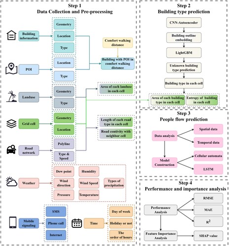
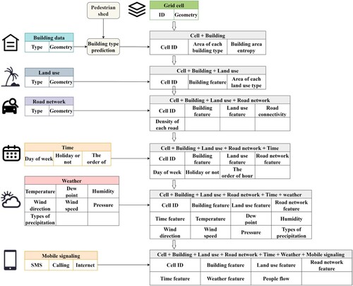
As shown in Figure 1, the study comprises four parts: (1) data collection and pre-processing, (2) building type prediction, (3) population distribution prediction, and (4) performance and importance analysis. In the first part, eight types of data – building, POI, land use, spatial grid, road, weather, mobile phone signalling, and time – were collected from four data sources. Next, building information was enriched by combining it with a POI within a comfortable walking distance; land use, road network, and mobile phone signalling data were allocated according to grid cells; and weather data were reorganised and aligned with mobile phone signalling data according to their temporal resolution. Finally, data analysis was applied to explore the correlation between mobile phone signalling and other data. Considering that building type is not available in all building information, it was predicted based on the building’s typology and its surrounding POIs. Convolutional autoencoder (CAE) was used to estimate the one-dimensional representation of the building outline without losing excessive information. Next, this representation was combined with POIs within a comfortable walking distance from the building as the input for LightGBM to predict unknown building types. The third part introduced a hybrid method integrating CA and LSTM to predict population distribution (indicated by mobile phone signalling) based on building, land use, road network, and weather conditions. Finally, the model's performance was analysed and compared with that of other ML models, and a feature importance analysis was conducted to highlight the contribution of each feature.

Figure 1. Framework of this study.

3.1. Data collection and pre-processing

In section 2.1, several influencing factors are summarised, but no study comprehensively compares the influence of all factors in population distribution prediction. The study area is Milan, the second-largest city in Italy. Milan covers 181.67 km² and had more than 1.37 million residents in 2019. The Italian government has been devoted to the development of open data; therefore, the data used in this study were collected from four publicly available sources (Table 2). POI, building, and road data in this study were collected from OpenStreetMap (https://www.openstreetmap.org), an open-source, editable map service that provides detailed geographic data. POI data consist of location and type; building data comprise location, outline, and building type; and road network consists of shape and type. As shown in Figure 2, the road network in Milan is similar to a spider web. Most footways are in the city centre, and track roads are distributed in the periphery of city.

Figure 2. Road network of Milan.

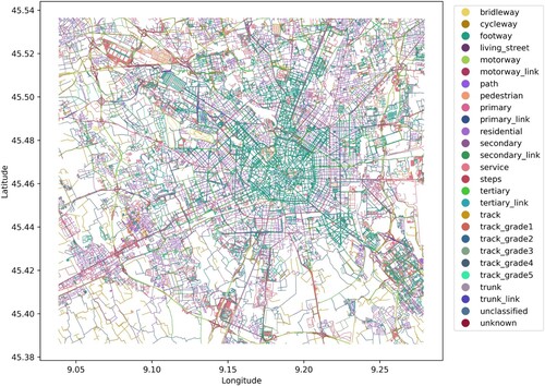
Table 2. Details of collected data

Name	Explanation	Type
POI	Position, type of each POI	Point
Building	Position, shape and type of each building	Geometry
Road	Position, shape and type of each road	Line
Land use	Position, shape and type of land use	Geometry
Weather	Seven weather factors for each hour	String/Continuous
Mobile phone signalling	The number of mobile signalling in each cell and each hour	Integer
Grid cell	Position and shape of each 235m × 235 m cell	Geometry

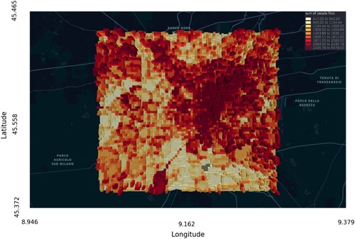
Land use data in 2012 were collected from Copernicus (https://land.copernicus.eu), the European Union's Earth observation programme. It provides data on land, the marine environment, climate change, emergency management, and security. Land use data for Milan shows that residential areas, leisure, and public services are mainly located in the city centre, and agricultural and industrial areas are located in suburban areas (Figure 3). European Centre for Medium-Range Weather Forecasts (ECMWF, https://www.ecmwf.int) records historical weather information worldwide each hour. The weather information comprises temperature, dew point, humidity, wind direction, wind speed, pressure, and types of precipitation. Mobile phone signalling data were collected from the mobile phone usage activity dataset issued by the Telecom Italia Big Data Challenge 2014. It records all received and sent short messages, incoming and outgoing calls, and internet usage activity every hour in Milan. Mobile signalling is a sampling data, but the ratio of coverage is large according to World Bank. The data has been widely used in human behaviour analysis (Barlacchi et al. 2015; Chin et al. 2019; Liu, Long, et al. 2021). In this study, mobile signalling was used as population distribution. Weather and mobile phone signalling were collected from 2013-11-01–2013-11-07, and the temporal granularity was processed to be one hour. Data publisher divided Milan and its neighbouring areas into 5680 square grid cells, and the size of each grid cell was 235 m × 235 m. Figure 4 shows the total population distribution for seven days in Milan. The figure indicates that most people are located in city centres and surrounding towns.

Figure 3. Distribution of land use in Milan.

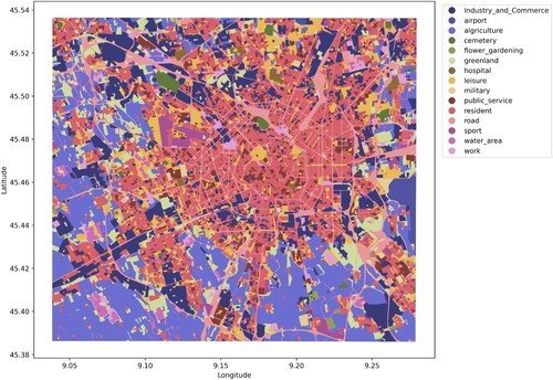
Figure 4. Distribution of one week of mobile phone usage in Milan as a high-resolution grid cell.

Figure 5 depicts the data pre-processing steps. For building data, the percentage of each building type occupied in every grid cell was calculated, and entropy was introduced to represent the diversity of building types in each cell. High entropy reflects a diversified building type in that cell and indicates a high-level neighbourhood activity (Huang et al. 2021). For land use, the area of each land use type was subdivided into each grid cell, and more land use types in each grid cell reflect a higher level of diversity of people’s behaviour patterns. The road network is another crucial factor, and its connectivity is derived to reflect the possible mobility with neighbouring cells. It is defined as the number of roads connected to the neighbouring grid cells. Next, each road density was also calculated for each cell. Other data used to predict population distribution include the day of the week, holidays, and the order of hours in a day.

Figure 5. Data pre-processing workflow.

3.2. Building type prediction

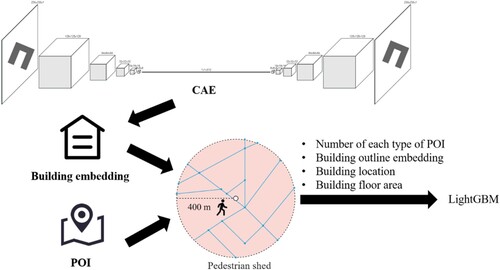
As discussed in Section 2, buildings play a crucial role in shaping human behaviour. In this section, unknown building types (nearly 30%) were predicted in the dataset. Building type prediction involves building features and associated surrounding environments. Using building images alone may lead to low prediction accuracy (Hoffmann, Abdulahhad, and Zhu 2022); hence, building outline and neighbouring POI data were combined for the prediction. The process can be divided into two parts: building outline embedding and building type prediction by surrounding POIs.

3.2.1. Building outline embedding

In this study, building outlines were selected as features for predicting building types, and CAE was used to acquire a low-dimensional representation of building outlines. CAE is designed to extract image features and transform them into embeddings which include nearly all image information and can be used as input for ML methods. It uses convolution operations to preserve the positional relationship between image pixels, rendering it suitable for building outline extraction (Zhang 2018). CAE combines CNNs and autoencoders; it consists of a convolutional layer, max-pooling layer, and fully connected layer. It uses fewer parameters to capture the key characteristics of an image and consistently outperforms the backpropagation neural network. Autoencoders are unsupervised ML methods that map the input to a latent representation. Autoencoders apply the function $h=\sigma \left(Wx+b\right)$, where $\sigma$ is an activation function, $W$ is the parameters of the autoencoder, and $b$ is bias. Autoencoders reconstruct the input $x$ to $x^{\mathrm{\prime }}$ and attempt to reduce the difference between them.

CAE is widely used because of its strong ability to process images (Guo et al. 2017; Mirjalili et al. 2018; Suganuma, Ozay, and Okatani 2018). A CAE consists of two layers: encoder $f_E$ and decoder $f_D$, and it aims to minimise the mean squared error between its input and output. (1) $\begin{array}{c}\underset{D,E}{\mathrm{M}\mathrm{i}\mathrm{n}}{\displaystyle \frac{1}{n}\sum _{i=1}^n{f}_D\left(f_E\left(x_i\right)\right)-x_i{2}^2}\end{array}$(1) (2) $\begin{array}{c}{f}_E\left(x\right)=\sigma \left(W_{E}x+b_E\right)\equiv h\end{array}$(2) (3) $\begin{array}{c}{f}_D\left(h\right)=\sigma \left(W_{D}h+b_D\right)\end{array}$(3)

Where $x_i$ is the i^th input, $W_E$ and $W_D$ are the parameters of the encoder and decoder, respectively, and $b_E$ and $b_D$ are the biases of the encoder and decoder, respectively.

3.2.2. Building type prediction

The building type prediction process is illustrated in Figure 6. POI is an important feature that indicates the type of built environment and the influence of POIs on building type only takes effect within a certain distance from each building. Pedestrian shed is the distance which is 400 m that people prefer walking before driving or choosing public traffic, and it has been widely accepted as a comfortable walking distance (Weinstein Agrawal, Schlossberg, and Irvin 2008; Wolch, Wilson, and Fehrenbach 2005). In this study, POIs within a comfortable walking distance, building outline embeddings, location, and floor area are inputs to LightGBM.

Figure 6. Process of predicting building type.

LightGBM is a novel gradient-boosting decision tree algorithm suitable for classification problems. It uses an improved histogram algorithm to divide continuous values into k intervals, and the split points are selected from the k intervals. In addition, LightGBM uses leaf-wise strategy to improve accuracy and limit the growth depth. Gradient-based one-side sampling introduced in LightGBM only considers data with a large gradient to reduce computation cost. Finally, this method uses exclusive feature bundling to bind many mutually exclusive features into a single feature to achieve dimension reduction. Thus, unlike other gradient-boosting decision tree methods, LightGBM accelerates the training process without losing accuracy and has been widely used in classification and regression problems. Several studies have demonstrated the superiority of LightGBM compared with other tree-based models such as Random Forest and XGBoost (Huang 2021; Ke et al. 2017; Wang, Zhang, and Zhao 2017).

3.3. Population distribution prediction

This section introduces an integrated method combining CA and LSTM to predict population distribution. It can be concluded from Figure 4 that population distribution has aggregation effects; densely populated areas are surrounded by at least one or more densely populated areas, which is suitable for applying CA which is designed to model the effect of neighbouring areas of a cell. Population distribution is in the form of a typical time series, indicating that data in the current time step is highly correlated to the data in the past time step. Because of their specific design, LSTM can ‘memory’ past data to support the prediction of current data. Thus, LSTM is chosen as a significant component of the hybrid model.

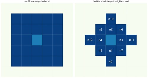
CA is one of the most widely used spatially explicit models to accurately capture spatial characteristics and simulate the law of natural evolution (Itami 1994). CA consists of four elements: (1) grid cells; (2) neighbourhood, neighbouring cells affect the change in the target cell; (3) the state of a cell, which indicates population distribution in this study; and (4) transition rules, which determine how neighbourhoods influence the state of the target cell. All cells change their states according to the rules at a time. The new states are added to the grid cells, and the procedure is repeated until the termination conditions are satisfied (Clarke 2014). Two elements need to be determined: neighbourhood and transition rules. For the neighbourhood, the most widely used neighbourhood is the Moore neighbourhood, whose shape is a rectangle, as shown in Figure 7(a); however, a diamond-shaped neighbourhood is more suitable in this study because the distance between the centre cell and each neighbour cell from different directions is equal, as shown in Figure 7(b). Optimised numbers of neighbourhoods are evaluated to improve computation efficiency without losing accuracy. The transition rule has a significant impact on prediction performance because such a rule represents how the state of a cell changes according to its neighbours’ states. An example of the transition rules is Game of life., Transition rules are summarised as follows:

1. If a cell is surrounded by three live cells, in the next time step, the cell’s state is live.

2. If a cell is surrounded by two live cells, in the next time step, the cell’s state does not change.

3. Under other conditions, this cell’s state is death in the next time step.

   More details of Game of life can be found in (Adamatzky 2010).

   Figure 7. Example of (a) Moore and (b) diamond-shaped neighbourhood.

   

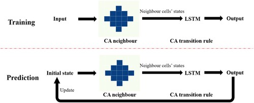
LSTM is a practical, scalable ML model for time series data, with a solid capability to learn temporal characteristics (Greff et al. 2016). The most crucial part of LSTM is the memory cell that remembers information from the past. In this study, LSTM receives states of neighbour cells including building, land use, road, time and weather data are shown in Figure 5. The output is the predicted population distribution of the target cell.

The process of combining LSTM and CA is illustrated in Figure 8. CA can be seen as an upper-level framework of the hybrid model, it defines the neighbouring cells to be considered and their interaction, which enables the model to consider spatial information. The transition rule in our model is not as simple as that in Game of Life, so LSTM can be seen as a method to construct a complex transition rule. In the training process, the state of each cell at a time step includes data on building, land use, road, weather, time, and population distribution. The inputs of LSTM are neighbouring cells’ states and the label is population distribution which is used to update the states of central cell. In the prediction process, the model first predicts population distribution using states of neighbouring cells, then the result updates the initial state, and the model starts to predict again. The process iterates until the termination rule is satisfied.

Figure 8. Process of combing CA and LSTM.

3.4. Prediction performance

Two performance indexes were used for building type prediction: accuracy and F1-score. Accuracy is the ratio of correctly classified samples to the total samples. F1-score evaluates precision and recall, and the weighted-average method is used to calculate precision and recall. Formulas for the two indexes are as follows: (4) $\begin{array}{c}\mathrm{A}\mathrm{c}\mathrm{c}\mathrm{u}\mathrm{r}\mathrm{a}\mathrm{c}\mathrm{y}=\sum _{i=1}^{n_t}T{P}_i/M_s\end{array}$(4) (5) $\begin{array}{c}{F}_1=2\times P\times R/\left(P+R\right)\end{array}$(5) (6) $\begin{array}{c}P=\sum _{i=1}^{n_t}{\displaystyle \frac{T{P}_i}{T{P}_i+F{P}_i}\cdot {\displaystyle \frac{m_i}{M_s}}}\end{array}$(6) (7) $\begin{array}{c}R=\sum _{i=1}^{n_t}{\displaystyle \frac{T{P}_i}{T{P}_i+F{N}_i}\cdot {\displaystyle \frac{m_i}{M_s}}}\end{array}$(7) where $n_t$ is the number of types, $T{P}_i$ is the number of correct predictions of type i, $M_s$ is the number of samples, $F{P}_i$ is the number of incorrect predictions of type i, $m_i$ is the number of type i, and $F{N}_i$ is the number of samples incorrectly predicted as type i.

Three performance indices were used for population distribution prediction: root mean squared error (RMSE), mean absolute error (MAE), and R². RMSE represents the standard deviation of the residuals between the predicted and observed population distributions. MAE is the mean value of the absolute difference between the predicted and observed values. R² is the ratio between the sum of regression square to total deviation square, which reflects the degree of fit of the model to the data. The formulas for the three indices are as follows: (8) $\begin{array}{c}RMSE=\sqrt{\sum _{i=1}^N{\left({\hat{Y}}_i-Y_i\right)}^2/N}\end{array}$(8) (9) $\begin{array}{c}MAE={\displaystyle \frac{1}{N}\sum _{i=1}^N{\widehat{|Y}}_i-Y_i|}\end{array}$(9) (10) $\begin{array}{c}{R}^2=1-\sum _1^N{\left({\hat{Y}}_i-Y_i\right)}^2/\sum _1^N{\left(\overline{Y}-Y_i\right)}^2\end{array}$(10) where ${\hat{Y}}_i$ is the predicted value of the $i^{th}$ sample, $Y_i$ is the true value of the $i^{th}$ sample, N is the number of samples, and $\overline{Y}$ is the average value of $Y_i$.

3.5. Variable importance analysis

Analysing the importance of each variable is necessary to deepen the understanding of their contribution to prediction performance. This study applied a feature importance analysis method, namely Shapley additive explanation (SHAP).

SHAP describes the performance of an ML method based on game theory. It defines the output model as the linear addition of each input variable, and the formula is shown as follows: (11) $\begin{array}{c}f\left(x\right)=g\left(x^{\mathrm{\prime }}\right)={\varphi }_0+\sum _{i=1}^M{\varphi }_i{x}_i^{{}^{\mathrm{\prime }}}\end{array}$(11) where $f\left(x\right)$ is the original model, $g\left(x^{\mathrm{\prime }}\right)$ is the explanation model, $x^{\mathrm{\prime }}$ is calculated by $x$ via a mapping function: $x=h_x\left(x^{\mathrm{\prime }}\right)$, $x=\left(x_1,x_2,\dots ,x_M\right)$, M is the number of variables, and ${\varphi }_i$ is the parameter. According to (Lundberg and Lee 2017), there is only one solution for ${\varphi }_i$ in Equation (11), and it has three desirable properties.

Property 1. (Local accuracy): The explanation model $g\left(x^{\mathrm{\prime }}\right)$ matches the original model $f\left(x\right)$ when $x=h_x\left(x^{\mathrm{\prime }}\right)$, where ${\varphi }_0$ = $f\left(h_x\left(0\right)\right)$ represents the model output with all simplified inputs toggled off.

Property 2. (Missingness): If the input feature is $x_i^{{}^{\mathrm{\prime }}}$ = 0, its importance is ${\varphi }_i$ = 0.

Property 3. (Consistency): If a model is changed to increase the impact of the variable, the importance of the feature never decreases.

With three properties, ${\varphi }_i$ can be calculated using the following formula: (12) $\begin{array}{c}{\varphi }_i\left(f,x\right)=\sum _{z^{\mathrm{\prime }}\subseteq x^{\mathrm{\prime }}}{\displaystyle \frac{\left|{\mathit{z}}^{\mathrm{\prime }}\right|!\left(M-\left|z^{\mathrm{\prime }}\right|-1\right)!}{M!}\left[f_x\left(z^{\mathrm{\prime }}\right)-f_x\left(z^{\mathrm{\prime }}\mathrm{\setminus }i\right)\right]}\end{array}$(12) where $z^{\mathrm{\prime }}\mathrm{\setminus }i$ represents $z_i^{{}^{\mathrm{\prime }}}=0$. $\left|{\mathit{z}}^{\mathrm{\prime }}\right|$ is the number of non-zero entries in ${\mathit{z}}^{\mathrm{\prime }}$, $z^{\mathrm{\prime }}\subseteq x^{\mathrm{\prime }}$. ${\varphi }_i$ is the Shapley values. Lundberg and Lee proposed SHAP values, which are the Shapley values of a conditional expectation function of the original model and approximated by combining the ideas of the additive feature attribution method. Details of the Shapley values and its approximation are available in Lundberg and Lee (2017).

Among the five methods for SHAP value calculation, the expected gradient, an extension of the integrated gradients method (Lundberg and Lee 2017), is the most suitable for deep ML methods. It is based on an extension of Shapley values to infinite player games (Aumann–Shapley values). This study applied the expected gradient to analyse the contribution of each variable.

6. Results and discussion

6.1. Building type prediction

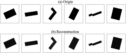
Each building outline was presented as a picture of size 256 × 256 × 1 to preserve image quality and facilitate CAE processing. The CAE was used to transform these pictures into embeddings. The structure of the CAE is illustrated in Figure 9. There are five layers in the CAE, and for each layer, batch normalisation was applied to avoid gradient vanishing and explosion. A parametric rectified linear unit was selected as the activation function. Examples of the reconstruction are shown in Figure 10.

Figure 9. Structure of CAE.

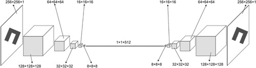
Figure 10. Examples of (a) building outlines and (b) their reconstruction.

As mentioned in Section 3.2.2, building outline embeddings and POI information within pedestrian sheds were used as inputs to LightGBM for building type prediction. This study applied a 3-fold grid search to determine the optimal parameters of LightGBM, including the number of leaves, maximum depth, and learning rate. Table 3 shows the range of the grid search and the optimal parameters.

The ratio of the training and testing sets was 7:3, the F1-score was 0.902, and the accuracy was 86.8%. Figure 11 shows the prediction outcome of building distribution in Milan.

Figure 11. All building distribution in Milan after prediction.

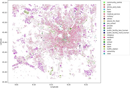
Table 3. Setting and result of LightGBM.

Name of parameters	The range of parameters	Optimal parameter
Number of leaves	20, 50, 100, 200, 350, 500, 800, 1000	500
Max depth	5, 10, 20, 40, 60, 80, 100	40
Learning rate	0.002, 0.004, 0.006, 0.008,0.1	0.004

The ratio of the training and testing sets was 7:3, the F1-score was 0.902, and the accuracy was 86.8%. Figure 11 shows the prediction outcome of building distribution in Milan.

6.2. Data analysis

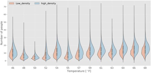
Figure 12 depicts the relationship between temperature, building density, and population distribution, the red part (left part) is the distribution of people number for low-density building in different temperatures, the blue part (right part) is the distribution of people number for high-density building in different temperature. A low density indicates that the area covered by buildings is below 1% of that of the grid cell, and a high density indicates that the area of buildings is larger than 20% of that of the grid cell. The choice of low and high density of threshold is according to 25th and 75th quantiles. The number of people is higher in high-density building areas than that in low-density building areas. Mann–Whitney U test was used to compare differences between two data distribution. p-values for all temperatures are smaller than 0.05 (from 0 to 1.98 × 10⁻⁹²), which indicates that there is a difference between population distribution in high-density building areas and low-density building areas for all temperatures.

Figure 12. Relationship between temperature, building density, and population distribution.

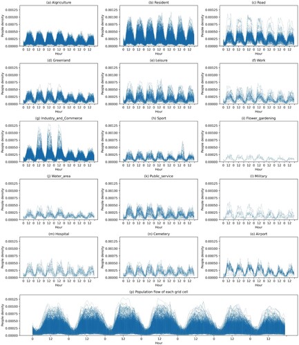
Figure 13(a–o) depicts the population distribution in different land use areas. Each line indicates that the area of land use is more than 70% of the area of the grid cell. The first four days were working days, and the last three days were All Saints holidays. For most areas, working days show similar patterns, and the population distribution during holidays is lesser, especially during the daytime. In addition, in areas with fixed behavioural patterns, such as residential, agricultural, and public service areas, population distribution is more stable than in areas with high personnel mobility, such as airports and hospitals. Moreover, work, residents, and road-related areas have a higher population distribution than other areas. For comparison, Figure 13(p) shows the population distribution of each grid cell. Without considering land use, the difference between workdays and holidays and the daily behaviour of people in different grid cells are difficult to summarise.

Figure 13. Population distribution of various land use (a–o) and grid cells (p).

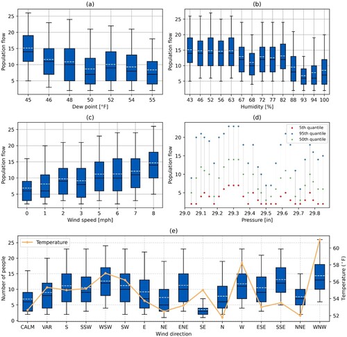
Figure 14 shows the dew point, humidity, wind speed, pressure, and population distribution for weather data. Population distribution is inversely proportional to dew point and humidity shows a similar pattern to dew point. However, wind speed is proportional to population distribution. The relationship between pressure and population distribution is more complicated, and the highest population distribution occurs when pressure is approximately 29.3 in. Hg. Figure 14(e) indicates that various wind direction and temperature significantly impacts population distribution.

Figure 14. Relationship between dew point (a), humidity (b), wind speed (c), pressure (d), temperature, wind direction (e), and population distribution; the black line is the median value, and the white line is the mean value.

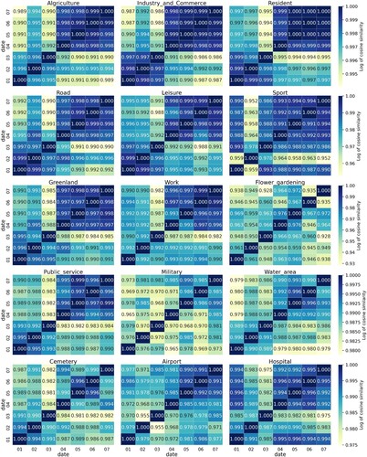
The cosine similarity of grid cells on different days of the week was implemented on several types of land use (Figure 15). For most areas except military and flower gardens, the patterns in the first three days are similar because of the All-Saints holidays; the last four days show another pattern because they are workdays. Thus, holidays are another important factor that should be included in the model.

Figure 15. Cosine similarity between grid cells on days of a week for land use types.

6.3. Population distribution prediction

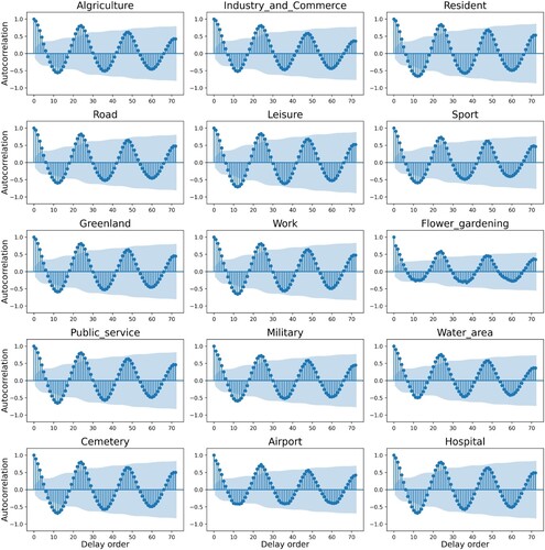
As introduced in Section 3.3, a hybrid method combining CA and LSTM was used to predict population distribution. This study applied Bi-LSTM because it captures the combined information of the input sequence in the forward and backward directions. A fully connected layer follows the two Bi-LSTM. Another important parameter of Bi-LSTM is the time step, which was determined by autocorrelation in this study. Autocorrelation measures the similarity of a particular time signal with itself on a time scale (Roy, Dey, and Chatterjee 2020). The similarity reflects that the number of prior points can be used to explain the current point. The formula is as follows: (13) $\begin{array}{c}ACF\left(k\right)={\displaystyle \frac{{\sum }_{i=1}^{N-k}\left(x\left(i\right)-\overline{x}\right)\left(x\left(i+k\right)-\overline{x}\right)}{{\sum }_{i=1}^N{\left(x\left(i\right)-\overline{x}\right)}^2}}\end{array}$(13) where $x\left(i\right)$ is the original dataset, $i$ is the time point, $k$ is the time lag, $\overline{x}$ is the mean value of the dataset, and $N$ is the number of time points. Figure 16 shows the result of the autocorrelation of all grid cells, where the blue area is the 95% confidence interval. Figure 16 indicates that the lag of all grid cells is 4. Therefore, 4 was chosen as the time step in Bi-LSTM.

Figure 16. Autocorrelation of population distribution for grid cells in different land use types.

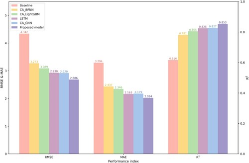
In this study, five models were compared with the proposed integrated model. The first model used the mean value of the previous four hours’ population distribution as the baseline; because CA is mostly used to predict discrete variables, it is difficult to determine the transition rule when predicting continuous variables using CA. ML methods are used to learn the complicated transition rule, and the most widely used method is the backpropagation neural network (BPNN). Thus, the second model used the combination of CA and BPNN, which considers less temporal information than the first model. The combination of CA and convolutional neural network (CNN) are used as the third model and the fourth model is the combination of CA and LightGBM which is a tree-based model. The fifth model only used LSTM, which disregards spatial relationships. Six-day records were used for training. The input information includes building footprint, build type, land use, road, time, and weather, and the population number is the model’s output. Observations on the last day were used for validation using the evaluation methods introduced in Section 3.4. All models are applied cross-validation to find the optimal parameters to avoid underfitting and overfitting. The training process of proposed model and model performances are shown in Figures 17 and 18; the proposed model outperformed other popular models in terms of RMSE, MAE, and R². Thus, the proposed method, which integrates model-based and ML mechanisms, improves the performance of population distribution prediction.

Figure 17. Training process of proposed model.

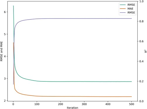
Figure 18. Comparison of proposed model and other three models (baseline, CA + BPNN, and LSTM)

6.4. Variable importance analysis

As introduced in Section 3.5, SHAP was used to qualify the contribution of each influencing variable. All variables were divided into seven categories: neighbour, historical information, weather, land use, building, road, and current time information. The neighbour category consists of neighbour information and the location of the current grid cell. The historical information category includes population distribution in the four previous steps (t-1 to t-4). The current time consists of holidays and the order of hours. Information on the importance of the 35 most important variables is presented in Figure 19. The order of hours is the most significant variable, with a significance of 0.224. Historical data also have a significant effect on population distribution because all historical variables are ranked high (larger than 0.04) and their contribution decreases from t-1 to t-4.

Figure 19. Importance of each variable (n1 to n12 refers to the code of neighbour cells shown in Figure 7).

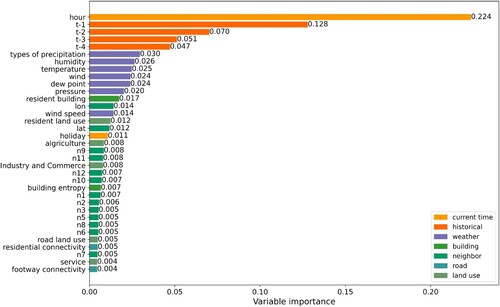
Types of precipitation are the most important factor in weather-related variables, followed by humidity, temperature, wind direction, dew point, and pressure. Wind speed is the least important factor.

Resident-related variables, including residential building, residential land use, and resident road, are more important than other variables for building, land use, and road category, which indicates that population distribution is closely related to housing-related factors. For neighbour data, the location of the grid cell is the most important, and the farther neighbouring cells are more important than the closer ones because people can travel a long distance within an hour. Notably, the connectivity of roads with neighbouring cells plays a more significant role in predictions than other road-related variables because the movement of people between areas is highly dependent on roads.

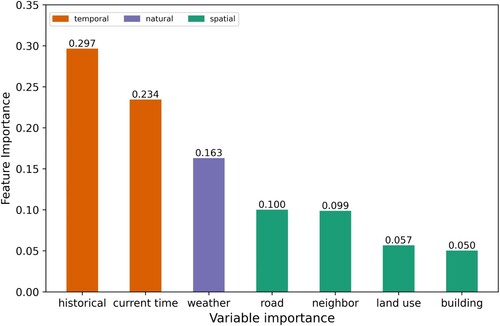
In addition, a more comprehensive analysis was conducted, and the seven categories above were divided into spatial-related, temporal-related, and natural-related variables (Figure 20). A comparison shows that historical information is the most important category, accounting for 29.7% of the contribution to performance because the movement of people is closely related to data in prior times (Section 4.3). The importance of current time and weather data rank second and third, respectively. The least important category is building, followed by land use, and their importance is less than 10%. Temporal variables are the most important category, whose importance is 0.531, followed by temporal and natural variables. The importance of temporal variables can be explained by the system of practice (Eon et al. 2018), system of practice indicates that a routine can be formed through the continual reproduction of everyday practices. The trip rules such as commuting demand and individual travel preference can be seen as a system of practice, that means people prefer to travel to a certain place at a certain time, which improve the importance of temporal features. In addition, the population distribution is a time-series data which has the characteristic of continuity. Thus, the population distribution at current hour is highly dependent on that in previous hours.

Figure 20. Importance of each category.

The available spatial data in Milan are ideal for modelling population distribution, which is, however, not common for other cities. If the hybrid model was applied to these cities, the analysis conducted in this study would provide a guidance on what type of data should be accorded more attention and how the model may perform with missing data. Solving these issues may show the ways to improve the transferability of the proposed model.

7. Conclusion and discussion

In this study, we proposed a hybrid model combing CA and LSTM to predict high spatial and temporal resolution population distributions. The proposed method addressed the limitations of previous methods, such as the low accuracy of conventional methods, the low interpretability of ML methods, and the high dependence on prior knowledge required by model-based methods. Multi-source data in Milan, Italy, were collected to validate the model. First, CAE, which extracts the embedding information of building outlines, was combined with LightGBM to predict unknown building types. Next, building information, land use, road network, weather, and time were collected and analysed to understand the relationship between the selected variables and population distribution. Subsequently, a hybrid method combining CA and LSTM, which considers spatial and temporal information, was adopted to predict population distribution. Finally, a variable importance analysis based on the SHAP value showed the importance of each variable, and the contribution of all variables was ranked based on their SHAP values.

The major findings are summarised as follows:

1. Building type prediction indicates that considering building outlines, POI information, and pedestrian sheds can achieve satisfactory performance.

2. Compared with CA + BPNN and LSTM, the combination of CA and LSTM considering spatial and temporal information improves prediction accuracy by approximately 5%–10%.

3. Variable importance analysis shows that temporal data are the most important in prediction, and natural data are the least important. The order of hours has the highest importance of temporal data in all variables. In the spatial category, housing-related variables are more important. In addition, types of precipitation contribute the most to predictions in the natural category.

The outcomes of this research can provide the basis for improving the accuracy of population distribution prediction and help in variable selection for further research. In contrast with prior deep learning-based population prediction models, the mechanism and outcomes of this study can be explained. This work can also provide a guidance on the type of data that should be prioritised in population distribution prediction. The proposed model approves that the combination of model-based and machine learning methods improves the prediction performance of population distribution. The evolutionary mechanism makes CA suitable for predicting population distribution and LSTM learn the complex transition rule. A variable importance analysis quantifies the importance of influencing factors introduced in previous studies.

Although the proposed model shows satisfying performance, RMSE and MAE are larger than 2, which needs to be improved. Variable importance analysis shows that temporal information is the most important. Thus, more temporal information should be extracted to improve the performance. Feature extraction methods such as time-field and frequency-field analysis can be attempted to obtain time signatures of population distribution, which reflect temporal changes and population distribution patterns. They can be added in the model for future improvement. Mobile signalling is not a fully accurate estimation of population distribution, its accuracy can be affected by network failing and frequent phone using, government statistics such as mobile phone user proportion and average daily mobile phone usage will be used for calibration. The study only focuses on Milan as case study. Improving the generalisation capability of the model to achieve similar performance on other cities is important. In the study, the model should be trained again when it is used for other cities, which require high computation resources. Thus, transfer learning mechanisms such as fine-tunning can be added on LSTM in the proposed model in the future.

Data availability statement

The authors confirm that the data supporting the findings of this study are available within the article.

Disclosure statement

No potential conflict of interest was reported by the author(s).

References

- Adamatzky, Andrew. 2010. Game of Life Cellular Automata. Vol. 1. Bristol: Springer.
- Akagi, Yasunori, Takuya Nishimura, Takeshi Kurashima, and Hiroyuki Toda. 2018. “A Fast and Accurate Method for Estimating People Flow from Spatiotemporal Population Data.” Paper presented at the IJCAI.
- Alessandretti, Laura, Ulf Aslak, and Sune Lehmann. 2020. “The Scales of Human Mobility.” Nature 587 (7834): 402–407. doi:10.1038/s41586-020-2909-1.
- Barlacchi, Gianni, Marco De Nadai, Roberto Larcher, Antonio Casella, Cristiana Chitic, Giovanni Torrisi, Fabrizio Antonelli, Alessandro Vespignani, Alex Pentland, and Bruno Lepri. 2015. “A Multi-Source Dataset of Urban Life in the City of Milan and the Province of Trentino.” Scientific Data 2 (1): 1–15. doi:10.1038/sdata.2015.55.
- Bock, Hans Georg, Thomas Carraro, Willi Jäger, Stefan Körkel, Rolf Rannacher, and Johannes P Schlöder. 2013. Model Based Parameter Estimation: Theory and Applications. Vol. 4. Berlin: Springer Science & Business Media.
- Bzdok, Danilo, Naomi Altman, and Martin Krzywinski. 2018. “Statistics Versus Machine Learning.” Nature Methods 15 (4): 233–234. doi:10.1038/nmeth.4642.
- Chen, Jiandong, Wei Fan, Ke Li, Xin Liu, and Malin Song. 2019. “Fitting Chinese Cities’ Population Distributions Using Remote Sensing Satellite Data.” Ecological Indicators 98: 327–333. doi:10.1016/j.ecolind.2018.11.013.
- Chen, Xiaoxuan, Xia Wan, Fan Ding, Qing Li, Charlie McCarthy, Yang Cheng, and Bin Ran. 2019. “Data-driven Prediction System of Dynamic People-Flow in Large Urban Network Using Cellular Probe Data.” Journal of Advanced Transportation 2019. doi:10.1155/2019/9401630.
- Chin, Kimberley, Haosheng Huang, Christopher Horn, Ivan Kasanicky, and Robert Weibel. 2019. “Inferring Fine-Grained Transport Modes from Mobile Phone Cellular Signaling Data.” Computers, Environment and Urban Systems 77: 101348. doi:10.1016/j.compenvurbsys.2019.101348.
- Clarke, Keith C. 2014. “Cellular Automata and Agent-Based Models.” Handbook of Regional Science, 1217–1233. doi:10.1007/978-3-642-23430-9_63.
- Cooper, Crispin HV, Ian Harvey, Scott Orford, and Alain J Chiaradia. 2018. “Testing the Ability of Multivariate Hybrid Spatial Network Analysis to Predict the Effect of a Major Urban Redevelopment on Pedestrian Flows.” arXiv preprint arXiv:1803.10500. doi: 10.48550/arXiv.1803.10500.
- Devi, U., and R. Mohan. 2020. “Long Short-Term Memory with Cellular Automata (LSTMCA) for Stock Value Prediction.” In Data Engineering and Communication Technology, 841–848. Springer. doi:10.1007/978-981-15-1097-7_70.
- Duives, Dorine C, Guangxing Wang, and Jiwon Kim. 2019. “Forecasting Pedestrian Movements Using Recurrent Neural Networks: An Application of Crowd Monitoring Data.” Sensors 19 (2): 382. doi:10.3390/s19020382.
- Eagle, Nathan, Michael Macy, and Rob Claxton. 2010. “Network Diversity and Economic Development.” Science 328 (5981): 1029–1031. doi:10.1126/science.1186605.
- Eon, Christine, Xin Liu, Gregory M Morrison, and Joshua Byrne. 2018. “Influencing Energy and Water use Within a Home System of Practice.” Energy and Buildings 158: 848–860. doi:10.1016/j.enbuild.2017.10.053.
- González, Marta C., César A. Hidalgo, and Albert-László Barabási. 2008. “Understanding Individual Human Mobility Patterns.” Nature 453 (7196): 779–782. doi:10.1038/nature06958.
- Greff, Klaus, Rupesh K Srivastava, Jan Koutník, Bas R Steunebrink, and Jürgen Schmidhuber. 2016. “LSTM: A Search Space Odyssey.” IEEE Transactions on Neural Networks and Learning Systems 28 (10): 2222–2232. doi:10.1109/TNNLS.2016.2582924.
- Gu, Danan, Kirill Andreev, and Matthew E. Dupre. 2021. “Major Trends in Population Growth Around the World.” China CDC Weekly 3 (28): 604–613. doi:10.46234/ccdcw2021.160.
- Gu, Hengyu, Ziliang Liu, Tiyan Shen, and Xin Meng. 2019. “Modelling Interprovincial Migration in China from 1995 to 2015 Based on an Eigenvector Spatial Filtering Negative Binomial Model.” Population, Space and Place 25 (8): e2253. doi:10.1002/psp.2253.
- Guo, Xifeng, Xinwang Liu, En Zhu, and Jianping Yin. 2017. “Deep Clustering with Convolutional Autoencoders”. Paper presented at the International conference on neural information processing. doi:10.1007/978-3-319-70096-0_39.
- Hoffmann, Eike Jens, Karam Abdulahhad, and Xiao Xiang Zhu. 2022. “Using Social Media Images for Building Function Classification.” arXiv preprint arXiv:2202.07315. doi: 10.48550/arXiv.2202.07315.
- Huang, Guilin. 2021. “Missing Data Filling Method Based on Linear Interpolation and Lightgbm.” Paper presented at the Journal of Physics: Conference Series. doi:10.1088/1742-6596/1754/1/012187.
- Huang, Lida, Tao Chen, Yan Wang, and Hongyong Yuan. 2015. “Forecasting Daily Pedestrian Flows in the Tiananmen Square Based on Historical Data and Weather Conditions.” ISCRAM 18: 1315–1320.
- Huang, Xiao, Cuizhen Wang, Zhenlong Li, and Huan Ning. 2021. “A 100 m Population Grid in the CONUS by Disaggregating Census Data with Open-Source Microsoft Building Footprints.” Big Earth Data 5 (1): 112–133. doi:10.1080/20964471.2020.1776200.
- Itami, Robert M. 1994. “Simulating Spatial Dynamics: Cellular Automata Theory.” Landscape and Urban Planning 30 (1-2): 27–47. doi:10.1016/0169-2046(94)90065-5.
- Ke, Guolin, Qi Meng, Thomas Finley, Taifeng Wang, Wei Chen, Weidong Ma, Qiwei Ye, and Tie-Yan Liu. 2017. “Lightgbm: A Highly Efficient Gradient Boosting Decision Tree.” Advances in Neural Information Processing Systems 30: 3146–3154.
- Kim, B. S., and T. G. Kim. 2019. “Cooperation of Simulation and Data Model for Performance Analysis of Complex Systems.” International Journal of Simulation Modelling 18 (4): 608–619.
- Lenormand, Maxime, Miguel Picornell, Oliva G Cantú-Ros, Thomas Louail, Ricardo Herranz, Marc Barthelemy, Enrique Frías-Martínez, Maxi San Miguel, and José J Ramasco. 2015. “Comparing and Modelling Land use Organization in Cities.” Royal Society Open Science 2 (12): 150449. doi:10.1098/rsos.150449.
- Liu, Shaojun, Yi Long, Ling Zhang, and Hao Liu. 2021. “Semantic Enhancement of Human Urban Activity Chain Construction Using Mobile Phone Signaling Data.” ISPRS International Journal of Geo-Information 10 (8): 545. doi:10.3390/ijgi10080545.
- Liu, Xin, Joseli Macedo, Tao Zhou, Liyin Shen, Yilan Liao, and Yulin Zhou. 2018. “Evaluation of the Utility Efficiency of Subway Stations Based on Spatial Information from Public Social Media.” Habitat International 79: 10–17. doi:10.1016/j.habitatint.2018.07.006.
- Liu, Chi Harold, Chengzhe Piao, Xiaoxin Ma, Ye Yuan, Jian Tang, Guoren Wang, and Kin K Leung. 2021. “Modeling Citywide Crowd Flows using Attentive Convolutional LSTM.” Paper presented at the 2021 IEEE 37th International Conference on Data Engineering (ICDE). doi:10.1109/ICDE51399.2021.00026.
- Liu, Jiamin, Bin Xiao, Yueshi Li, Xiaoyun Wang, Qiang Bie, and Jizong Jiao. 2021. “Simulation of Dynamic Urban Expansion Under Ecological Constraints Using a Long Short Term Memory Network Model and Cellular Automata.” Remote Sensing 13 (8): 1499. doi:10.3390/rs13081499.
- Louail, Thomas, Maxime Lenormand, Oliva G. Cantu Ros, Miguel Picornell, Ricardo Herranz, Enrique Frias-Martinez, José J. Ramasco, and Marc Barthelemy. 2014. “From Mobile Phone Data to the Spatial Structure of Cities.” Scientific Reports 4 (1): 1–12. doi:10.1038/srep05276.
- Lu, Lili, Ching-Yao Chan, Jian Wang, and Wei Wang. 2017. “A Study of Pedestrian Group Behaviors in Crowd Evacuation Based on an Extended Floor Field Cellular Automaton Model.” Transportation Research Part C: Emerging Technologies 81: 317–329. doi:10.1016/j.trc.2016.08.018.
- Lu, Zhenyu, Jungho Im, Lindi Quackenbush, and Kerry Halligan. 2010. “Population Estimation Based on Multi-Sensor Data Fusion.” International Journal of Remote Sensing 31 (21): 5587–5604. doi:10.1080/01431161.2010.496801.
- Lundberg, Scott M, and Su-In Lee. 2017. “A Unified Approach to Interpreting Model Predictions.” Paper presented at the Proceedings of the 31st international conference on neural information processing systems.
- Lutz, Wolfgang, Warren Sanderson, and Sergei Scherbov. 1997. “Doubling of World Population Unlikely.” Nature 387 (6635): 803–805. doi:10.1038/42935.
- Mahmoud, Amira. 2018. “The Impact of Built Environment on Human Behaviors.” International Journal of Environmental Science & Sustainable Development 3 (1). doi:10.21625/essd.v2i1.157.g69.
- Mirjalili, Vahid, Sebastian Raschka, Anoop Namboodiri, and Arun Ross. 2018. Semi-adversarial networks: Convolutional autoencoders for imparting privacy to face images. Paper presented at the 2018 International Conference on Biometrics (ICB). doi:10.1109/ICB2018.2018.00023.
- Mourad, Lablack, Heng Qi, Yanming Shen, and Baocai Yin. 2019. “ASTIR: Spatio-Temporal Data Mining for Crowd Flow Prediction.” IEEE Access 7: 175159–65. doi:10.1109/ACCESS.2019.2950956.
- Okwuashi, Onuwa, and Christopher E Ndehedehe. 2021. “Integrating Machine Learning with Markov Chain and Cellular Automata Models for Modelling Urban Land use Change.” Remote Sensing Applications: Society and Environment 21: 100461. doi:10.1016/j.rsase.2020.100461.
- Reichstein, Markus, Gustau Camps-Valls, Bjorn Stevens, Martin Jung, Joachim Denzler, and Nuno Carvalhais. 2019. “Deep Learning and Process Understanding for Data-Driven Earth System Science.” Nature 566 (7743): 195–204. doi:10.1038/s41586-019-0912-1.
- Robinson, Caleb, Fred Hohman, and Bistra Dilkina. 2017. “A Deep Learning Approach for Population Estimation from Satellite Imagery.” Paper presented at the Proceedings of the 1st ACM SIGSPATIAL Workshop on Geospatial Humanities. doi:10.1145/3149858.3149863.
- Roy, S. S., S. Dey, and S. Chatterjee. 2020. “Autocorrelation Aided Random Forest Classifier-Based Bearing Fault Detection Framework.” IEEE Sensors Journal 20 (18): 10792–10800. doi:10.1109/JSEN.2020.2995109.
- Suganuma, Masanori, Mete Ozay, and Takayuki Okatani. 2018. “Exploiting the Potential of Standard Convolutional Autoencoders for Image Restoration by Evolutionary Search.” Paper presented at the International Conference on Machine Learning. doi:10.1109/JSEN.2020.2995109.
- Vu, Long, Quang Do, and Klara Nahrstedt. 2011. “Jyotish: A Novel Framework for Constructing Predictive Model of People Movement from Joint Wifi/Bluetooth Trace.” Paper presented at the 2011 IEEE international conference on pervasive computing and communications (PerCom). doi:10.1109/PERCOM.2011.5767595.
- Wang, Dehua, Yang Zhang, and Yi Zhao. 2017. “LightGBM: An effective miRNA Classification Method in Breast Cancer Patients.” Paper presented at the Proceedings of the 2017 International Conference on Computational Biology and Bioinformatics. doi:10.1145/3155077.3155079.
- Wang, Shuwei, Ronggui Zhou, and Lin Zhao. 2015. “Forecasting Beijing Transportation Hub Areas’s Pedestrian Flow Using Modular Neural Network.” Discrete Dynamics in Nature and Society 2015. doi:10.1155/2015/749181.
- Weinstein Agrawal, Asha, Marc Schlossberg, and Katja Irvin. 2008. “How Far, by Which Route and Why? A Spatial Analysis of Pedestrian Preference.” Journal of Urban Design 13 (1): 81–98. doi:10.1080/13574800701804074.
- Wolch, Jennifer, John P Wilson, and Jed Fehrenbach. 2005. “Parks and Park Funding in Los Angeles: An Equity-Mapping Analysis.” Urban Geography 26 (1): 4–35. doi:10.2747/0272-3638.26.1.4.
- Yuan, Jing, Yu Zheng, and Xing Xie. 2012. “Discovering Regions of Different Functions in a City Using Human Mobility and POIs.” Paper presented at the Proceedings of the 18th ACM SIGKDD international conference on Knowledge discovery and data mining. doi:10.1145/2339530.2339561.
- Zakria, M., and F. Muhammad. 2009. “Forecasting the Population of Pakistan Using ARIMA Models.” Pakistan Journal of Agricultural Sciences 46 (3): 214–223.
- Zhang, Yifei. 2018. “A Better Autoencoder for Image: Convolutional Autoencoder.” Paper presented at the ICONIP17-DCEC. Accessed March 23, 2017. http://users.cecs.anu.edu.au/Tom.Gedeon/conf/ABCs2018/paper/ABCs2018_paper_58.pdf.
- Zhao, Miaoxi, Gaofeng Xu, Martin de Jong, Xinjian Li, and Pingcheng Zhang. 2020. “Examining the Density and Diversity of Human Activity in the Built Environment: The Case of the Pearl River Delta, China.” Sustainability 12 (9): 3700. doi:10.3390/su12093700.