Time-series surface water reconstruction method (TSWR) based on spatial distance relationship of multi-stage water boundaries

ABSTRACT

Spatiotemporal continuity of surface water datasets widely known for its significance in the surface water dynamic monitoring and assessments, are faced with drawbacks like cloud influence, which hinders the direct extraction of data from time-series remote sensing images. This study proposes a Time-series Surface Water Reconstruction method (TSWR). The initial stage of this method involves the effective use of remote sensing images to automatically construct multi-stage surface water boundaries based on Google Earth Engine (GEE). Then, we reconstructed regions the reconstruction of regions with missing water pixels using the distance relationship between the multi-stage water boundaries in previous and later periods. When applied to 10 large rivers around the world, this method yielded an overall accuracy of 98% for water extraction, an RMSE of 0.41 km². Furthermore, time-series reconstruction tests conducted in 2020 on the Lancang and Danube rivers revealed a significant improvement in the image availability. These findings demonstrated that this method could not only be used to accurately reconstruct the surface water distribution missing water images, but also to depict a more pronounced time variation characteristic. The successful application of this method on GEE demonstrates its importance for use on large scales or in global studies.

KEYWORDS:

• Google earth engine
• sentinel-2
• surface water reconstruction
• time-series surface water data

1. Introduction

Recently, global warming is widely known to be a causative factor for the occurrences of extreme weather events, which has resulted in frequent floods and rapid changes in the temporal and spatial distribution of surface water experienced globally (Schiermeier 2011; Huang and Swain 2022; Gu et al. 2020). The great changes in the global surface hydrological cycle, exacerbated by climate change (Huntington et al. 2018; Ficklin, Abatzoglou, and Novick 2019), pose challenges to traditional water resource management, so there is an urgent need for more effective surface water dynamic monitoring to support decision-making (Donchyts et al. 2016a; Wang et al. 2018). Time-series surface water data having the ability to fully reflect varying characteristics of regional water volume and providing a more effective data input for hydrological and meteorological models (Heimhuber, Tulbure, and Broich 2016; Ogilvie et al. 2018), have had significant influence in scientific research, water resource management, and sustainable socioeconomic development (Gao, Birkett, and Lettenmaier 2012), through its application in river runoff and lake water volume calculation (Feng et al. 2021; Gleason and Durand 2020; Liu et al. 2020).

Due to various advancements in remote sensing technology, with satellites revolving around the Earth at a distance of several hundred to thousands of kilometers, information acquired from sensors on board satellite systems serves as the most efficient source of time-series surface water mapping. One of the most widely used tools for large-scale spatiotemporal thematic mapping of remotely sensed images is a cloud platform for planetary-scale Earth science data and analysis known as Google Earth Engine (GEE) (Mou et al. 2021; Tamiminia et al. 2020; Gorelick et al. 2017). The GEE mainly contains three different types of optical satellite data: MODIS, Landsat, and Sentinel-2. The MODIS satellites have the highest temporal resolution, which develops water extents products with daily, 8-day and 16-day coverage (Soulard et al. 2022; Gao, Birkett, and Lettenmaier 2012; Lu et al. 2017; Khandelwal et al. 2017). While it possesses coarser spatial resolution, the small water bodies especially river (e.g. width less 100 m) may not accurately be discernible (Khandelwal et al. 2017). The Landsat satellites have unique advantages in long-term land surface monitoring due to their data continuity mission, which have helped the development of global monthly and annual surface water data products since 1985 (Pekel et al. 2016). The Sentinel-2 satellites have balanced temporal and spatial resolution and have also developed a variety of water-related data products (Ni et al. 2021; Bhangale et al. 2020; Du et al. 2016). Optical satellite images are widely used for water body extraction and monitoring changes (Huang et al. 2018). An easy and effective way to extract water is to use water indices. In 1979, Otsu proposed an automatic calculation of the threshold value by using the grayscale histogram (Otsu 1979). Since then, lots of local adaptive thresholding approaches have been developed with better water mapping (Li and Sheng 2012; Allen and Pavelsky 2015; Donchyts et al. 2016b). Machine learning (Huang et al. 2015; Li et al. 2021) and deep learning (John, Anderson Derek, and Chan Chee Seng 2017; Cheng et al. 2020) have been widely used. The features construction is very time-consuming and requires relevant expertise (Maxwell, Warner, and Fang 2018). Deep learning method can automatically extract features, but it is subject to the considerable difficulty of acquiring images of various water body types, as well as heavy labeling work (Isikdogan, Bovik, and Passalacqua 2017; Yuan et al. 2020; Bao, Lv, and Yao 2021).

Those approaches mentioned above are frequently hampered by clouds and cloud shadows, resulting in the loss of water pixels and a high number of no-data values in final products (we refer to such images in this study as contaminated images). According to the International Satellite Cloud Climatology Project, the global average annual cloud fraction could reach 66% (Zhang et al. 2004). These cloud presence severely affects the usability of images and impedes the exploration and analysis of real change characteristics (Li et al. 2022b). The Synthetic Aperture Radar (SAR) is a very effective tool for dealing with unfavorable weather conditions because of its ability to penetrate cloud cover. Because water has very low backscatter values on SAR images, it is possible to segment the water pixels by selecting a given threshold value (Chini et al. 2017). Furthermore, the continuous archive updating of the Sentinel-1 Ground Range Detected (GRD) data on GEE enhances its ability to reduce the complexity of SAR pre-processing (DeVries et al. 2020). Sentinel-1 has the potential for dynamic monitoring, mapping of water bodies on a large scale, and the development of a variety of water data products (Li et al. 2020a; Jiang et al. 2021). The surface water dataset consisting of classified permanent water, flood water, and raw Sentinel-1 images of SEN12MS and Sen1Floods11 can be used to train and test deep learning flood algorithms (Bonafilia et al. 2020; Schmitt et al. 2019).

Due to the restrictions of floating or seasonally emergent plants, excessive precipitation, and windy circumstances, the majority of proposed algorithms for contour extraction or texture analysis influence the SAR backscatter’s response to water bodies (López-Caloca et al. 2020; Martinis et al. 2015; Matgen et al. 2007). The application of sensor characteristics to resolve cloud influence for optical images that don't match the SAR images with the same date is futile. In terms of missing data, a pixel-scale medium or quality mosaic is typically used to restore them (Huang et al. 2017). When these images are used to inverse higher temporal resolution data(e.g. daily runoff), it is difficult to find enough images to create a mosaic image. Yao et al. (2019) recently recovered the value of contaminated image water area by simply interpolate, however they were unable to acquire precise inundation boundaries. Only the water body area value is available for rivers. The length of the river centerline can be used to estimate the average river width. However, calculating the river's width at a certain cross section is challenging. The precise inundation boundaries are essential for runoff estimation and river stability analysis because they make it easier to determine morphological characteristics, such as river width, and other variables. They also make it easier to comprehend how rivers evolve over time. Li et al. (2013) used elevations near the water to reconstruct the contaminated images where lower elevation pixels were filled. The resolution and accuracy of the Digital Elevation Model (DEM) is critical in water reconstruction, especially in lowlands areas where land elevation changes are typically only on the order of a few decimeters, and Shuttle Radar Topography Mission (SRTM) DEM has the accuracy on the order of meters (Jakovljević and Govedarica 2019). It also is challenging to determine precise water levels in a vast study area using DEM because, as a result of the hydraulic gradient, the elevation around the river lowers in the direction of the river flow (Wang et al. 2005). Global surface water data were used by Zhao and Gao (2018) to determine a water occurrence frequency threshold, which was then used to rectify contaminated pixels in water incidence image. Although the count threshold could be established using an empirical value (0.17), there was no technique for adapting the threshold's choice across different locations.

In order to bridge these gaps, the goal of this research is to create a Time-series Surface Water Reconstruction approach (TSWR) that will enable the creation of a spatiotemporal surface water data set using all available multi-spectral iamges. The missing water pixels brought on by clouds and cloud shadows will be recreated using the distance relationship between the polluted water border and multi-stage water boundaries recorded at various times. The accuracy and robustness of the technique will be evaluated using Sentinel-2 images of 10 distinct types of surface water bodies from around the world.

2. Data and methods

2.1. Remote sensing and global river widths data

With two satellite constellations, Sentinel-2 offers greater temporal (up to 5 days) and geographical resolutions (10m–20 m) (Misra, Cawkwell, and Wingler 2020). Hence, this study used Sentinel-2 images taken within a year to map the surface water boundaries and rebuild the water bodies, which could prevent changes in bank shape brought on by erosion and buildup (Boothroyd et al. 2021). Additionally, GEE provides direct access to all of the Sentinel-2 Multi-Spectral Instrument (MSI) L2A images. Figure S1 shows a summary of the data used in this study.

The Global River Widths from Landsat (GRWL) datasets, which combined satellite images (7,376 scenes of Landsat TM, ETM+, and OLI) and field measurements (3693 gauge stations) with statistical modeling to calculate worldwide river and stream center line location and width, including simplified vector, raw vector, and raster product, were used as the foundational data for estimating the surface area of rivers and streams (Allen and Pavelsky 2018). The datasets, which can be accessed at https://doi.org/10.5281/zenodo.1297434, were used in the water extraction post-process in this study.

2.2. Surface water reconstruction method

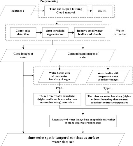
We proposed the Time-series Surface Water Reconstruction method (TSWR) in this study, which is based on the spatial distance relationship of multi-stage water boundaries. The algorithm's steps are as follows (flowchart shown in Figure 1):

1. From numerous Sentinel-2 images, map the surface water using an adaptive thresholding technique. In addition, the GRWL information was used to determine the main structure of the river.

2. Use those water boundaries of good images (images within the water body without any cloud or shadow pixels) as reference boundaries.

3. When the water boundary is only partially visible, the missing portion of contaminated images (images with blank pixels in the water-distributed area) is reconstructed using the distance relationship connection between the current and reference boundaries.

4. To create a dataset with a higher frequency of surface water, combine the reconstructed water images with the high-quality water images.

Figure 1. Flowchart of the algorithm for surface water reconstruction.

Section 2.2.1-2.2.3 provides a detailed explanation of the methodologies for surface water mapping, distance computation, and surface water reconstruction specified in the aforementioned phases.

2.2.1. Surface water mapping

The water information in this study was reflected by the water index, which was estimated using the reflectivity of different bands on optical images. According to the Sentinel-2 MSI sensor's band division, bands three and eight were selected to calculate the Normalized Difference Water Index (NDWI) (McFeeters 1996). Furthermore, we pre-processed the images with cloud pixels mask to eliminate the cloud effects for the NDWI mapping. (1) $NDWI=\left({\rho }_{Green}-{\rho }_{NIR}\right)/\left({\rho }_{Green}+{\rho }_{NIR}\right)$(1) where ${\rho }_{Green}$ is the green band; ${\rho }_{NIR}$ is the near infrared band.

After obtaining the NDWI, the Canny edge detection method was applied to identify the water and land junction in NDWI (Canny 1986). Then, applying the Otsu threshold segmentation method to extract the surface water as a water binary image (Otsu 1979).

In order to obtain the main river channel, small water bodies and small islands were removed. The approximate center point in GRWL was used as the source to construct a distance image, which calculates the shortest distance from each water pixel to the center point. GEE function ee.Image.cumulativeCost (source, maxDistance) was used to obtain the distance image, with a default maxDistance set at 1000 (the unit is a meter, this distance determination depends on the actual river width). The calculated distance that’s larger than the maxDistance was masked. Afterwards, small islands were removed using the connectivity image, where each pixel value was the number of 8-connected pixels. GEE function ee.Image.connectedPixelCount (maxSize) was used to obtain the connectivity image, with a default maxSize set as 100 (the unit is a pixel, this size determination depends on the spatial resolution of the remote sensing image). The pixels of islands less than the maxSize were reclassed to water. The maxDistance and maxSize parameters were modifiable, giving room to adjustments based on the prior knowledge of small water bodies and islands areas. Lastly, all the water boundaries extracted from all the good images were merged as the muti-stage water boundaries to reconstruct contaminated images.

2.2.2. Distance calculation

To ensure the center line was only one pixel wide, the binary water image was morphologically skeletonized and refined repeatedly (Jang & Chin, 1990). To create an orthogonal angle image, the river center line image was convoluted by a convolution core with an angle. The length of the double distance from the center line to the nearest land pixel was then used to produce a line segment (referred to as W) along the orthogonal direction. The intersection proportion of the W and the foreground in a water binarization image was determined using ee.Reduce.Mean in GEE. Afterward, the distance from the river center line along the orthogonal direction to the water boundaries was calculated by multiplying W with the proportion (Yang et al. 2020). Those distances were used to calculate the spatial relationship between the effective boundary in contaminated images and the reference water boundary in good images.

2.2.3. Reconstruction of surface water images

Water bodies were classified into two types based on algorithm implementation, such as Type I and Type II. Type I waterbodies had clearly defined water boundary changes. Their water boundaries gradually shrink inward as the water level drops. This type is commonly found in U- or V-shaped river cross-sections and river (lake or reservoir) levels that vary significantly throughout the year. Type II waterbodies had undetectable water boundary changes and short distances between multi-stage water boundaries, which were commonly found in rectangular cross-sections rivers. Rivers that flow downstream of artificially regulated reservoirs and rivers in cities, as well as some natural lakes with steep terrain.

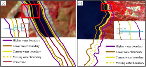
In this study, contaminated water pixels for Type I waterbodies were reconstructed using the higher and lower complete water boundary constraint. The water flow was assumed to be similar between two nearby areas (observed and obstructed), and the water-land interface line under a certain water level can be regarded as an elevation contour of the river bank. Figure 2a illustrates how, despite the incompleteness of the shorelines that were retrieved from contaminated pictures, the placement of these partial water borders nonetheless suggested that there was an elevation sequence between the water levels represented by the higher and lower boundaries. In addition, it can be assumed that the change in slope between the two adjacent water boundaries (the smallest unit of the water boundary sequence) showed a linear trend (Yao et al. 2019). As a result, the contaminated image's missing water boundary was linearly bound/enclosed by the higher and lower complete water boundaries. The missing water bodies were recovered using spatial interpolation to reduce the recovered area uncertainty. The distance relationship between the current water boundary and water boundaries in higher and lower water levels, as illustrated in equations, determined the interpolation coefficient k. (2-4). (2) $k={\displaystyle \frac{1}{2n}}$(2) (3) $x_{pi}=x_{ci}+cos\theta \left(l_l+k\left(l_h-l_l\right)\right)$(3) (4) $y_{pi}=y_{ci}+sin\theta \left(l_l+k\left(l_h-l_l\right)\right)$(4) where $k$ is the interpolation coefficient; $n$ is the number of pixels for center line; $D_1$and $D_2$ are the distances from the lower to the current water boundary and to the higher water boundary on one side of the center line with orthogonal direction, respectively (Figure 2a); $x_{pi}$ and $y_{pi}$ are the abscissa and ordinate of the $i$_th reconstructed water boundary point, respectively; $x_{ci}$ and $y_{ci}$ are the abscissa and ordinate of the $i$_th center line pixel, respectively; $\theta$is the orthogonal direction of the center line pixel; and $l_l$ and $l_h$ are the distance from the center line pixel to the lower and to the higher water boundary on one side of the center line orthogonal direction, respectively (Figure 2a).

Figure 2. Schematic diagram of the surface water reconstruction method: (a) the reconstruction method for river; (b) the reconstruction method for lake or reservoir; The image is Sentinel-2, and the band combination is B8 (near-infrared band), B4 (red band), and B3 (green band).

Following the reconstruction of the missing water boundary points, GEE also was used to convert them into raster images. The calculated boundary points were first connected to the corresponding center point, and the line images were resampled with the same resolution as the original image. Finally, the reconstructed water image was mosaiced from all connected line raster images. Following that, a post-processing analysis was performed to fill the internal empty pixels of the obtained raw image. First, the edge pixels with a single pixel width were separated from the raw mosaic raster. Then the internal raw mosaic image was then filled with morphological dilation, hole filling, and morphological erosion techniques (where the erosion is one step more than dilation).

For Type II water bodies with unapparent water boundary changes, the current water boundary was reconstructed based on the contraction/expansion higher or lower water boundaries with similar geometric characteristics in closer time range. The reconstructed water boundary position was calculated using distance relationship between the current water boundary and the reference water boundary (5-7). (5) $k={\displaystyle \frac{1}{n}\sum {\displaystyle \frac{D_1^{\mathrm{\prime }}}{D_2^{\mathrm{\prime }}}}}$(5) (6) $x_{pi}=x_{ci}+k\times l\times cos\theta$(6) (7) $y_{pi}=y_{ci}+k\times l\times sin\theta$(7)

Where $k$ is the interpolation coefficient; $n$ is the number of pixels for lower water boundary; $D_1^{\mathrm{\prime }}$ and $D_2^{\mathrm{\prime }}$ are the distances from the center line to the current and to the reference water boundary on one side of the center line orthogonal direction, respectively; $l$ is the distance from the center line to the reference boundary on one side of the center line orthogonal direction.

2.2.4. Reconstruction of lake and reservoir water images

Large water bodies like lakes and reservoirs have no clear direction of water flow, this makes the identification of center line impossible. Using similar principles applied in section 2.2.3 to calculate the position of the reconstructed boundary point. The interpolation coefficient k was calculated by the distance relationship between the orthogonal distances from the lower water boundary to current and higher boundaries, respectively (Figure 2b). By connecting all the reconstructed points with the corresponding lower lake boundary points and mosaicking the water raster of the lower water boundary, the reconstructed lake raster was obtained.

2.3. Accuracy evaluation method

To validate the surface water extraction method's applicability and accuracy. In this study, we used visual interpretation and quantitative analysis for verification. The comparison of the original image and the surface water mapping provided the visual interpretation. Following that, the visual interpretation of the original image was used to map validation labels (water/non-water). Furthermore, in the validation mapping, we chose small water as ‘non-water’ and islands as ‘water’ to validate the performance of the small water removal and island filling. Finally, the confusion matrix compares the actual and predicted categories. Using equations, the Overall Accuracy (OA) and Kappa coefficient were calculated using the rows and columns of the confusion matrix (8-10) (Rwanga and Ndambuki 2017; Li et al. 2020b; Becker et al. 2021). (8) $OA={\displaystyle \frac{TP+TN}{N}}$(8) (9) $Kappa={\displaystyle \frac{OA-\rho }{1-\rho }}$(9) where TP represents the number of correctly extracted water pixels, TN represents the number of correctly extracted non-water pixels, N represents the total number of pixels in the true value reference image, and ρ is the correlation coefficient, which can be expressed as: (10) $\rho ={\displaystyle \frac{\left(TP+FN\right)\left(TP+FP\right)+\left(TP+TN\right)\left(FN+TN\right)}{N^2}}$(10) where FP represents the number of wrongly extracted non-water pixels as water pixels, FN represents the number of wrongly extracted water pixels as non-water pixels.

We tested the reconstruction performance by the overall accuracy evaluation, the applications in Type I and II Water Bodies, and the time-series surface water reconstruction applications. The overall accuracy and applications in Type I and II water bodies performance was evaluated by comparing reconstructed water results obtained from the simulated contaminated image with the results obtained from the original good image. The simulated contaminated image was generated by randomly cropping a part from the good image (Zhao and Gao 2018; Yao et al. 2019). They were evaluated from two perspectives: (1) Inspecting the reconstructed results visually with the original good image, (2) quantitative evaluation indices between the reconstructed and real water area were calculated based on the slope of the linear fitting, Pearson Product-Moment Correlation Coefficient (PCC), and Root Mean Square Error (RMSE) illustrated in equations (11)(11) ${\rho }_{A_m,A_C}={\displaystyle \frac{cov\left(A_m,A_C\right)}{{\sigma }_{A_m}{\sigma }_{A_c}}}$(11) and (12)(12) $RMSE=\sqrt{{\left({\displaystyle \frac{\sum A_C-A_m}{n}}\right)}^2}$(12) (Mengen et al. 2020; Kebede et al. 2020). In the time-series surface water reconstruction applications, we validated the algorithm performance in those images that were truly contaminated by clouds. (11) ${\rho }_{A_m,A_C}={\displaystyle \frac{cov\left(A_m,A_C\right)}{{\sigma }_{A_m}{\sigma }_{A_c}}}$(11) (12) $RMSE=\sqrt{{\left({\displaystyle \frac{\sum A_C-A_m}{n}}\right)}^2}$(12) where ${\rho }_{A_m,A_C}$is the PCC between real water area and reconstructed water area; A_m is the real water area; A_c is the reconstructed water area; n is the total number of reconstructed senses.

3. Accuracy assessment

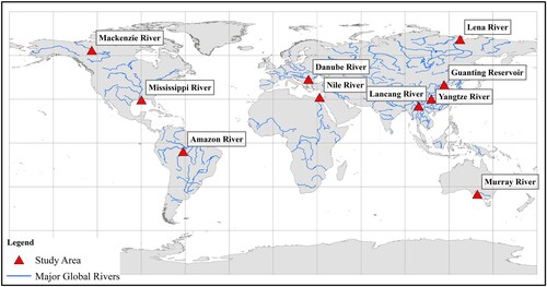
The Yangtze River, Lancang River, Lena River, and Guanting Reservoir in Asia; the Mississippi River and Mackenzie River in North America; the Murray River in Australia; the Amazon River in South America; the Nile River in Africa; and the Danube River in Europe were chosen as the experimental area to verify the algorithm's accuracy and robustness (Figure 3). Furthermore, the algorithm's accuracy was assessed using two river types with Type I (significant) and Type II (insignificant) changes in water boundaries, respectively. The running performance of the method was also evaluated in four challenging environments: high latitudes, cloudy and rainy weather, larger islands in river channels, and lake boundaries.

Figure 3. Location of the sample study areas

3.1. Accuracy of surface water extraction

Based on the validation study of the total 540 samples (Class 1 = water, Class 2 = non-water, Class 3 = small islands in the water with the validation label of water, and Class 4 = small water bodies on land with the validation label of water) randomly mapped from the 10 river sections, the OA and kappa coefficient of the water extraction were both 0.98. (Table 1). Seven validation samples were misclassified as belonging to class 1 based on the 215 samples in class 2, and they were all distributed throughout the mixed pixels at the water-land interface. The accuracy of surface water extraction results can be satisfied the construction of multi-stage water boundaries and the accuracy of surface water reconstruction.

Table 1. Confusion matrix between the extracted and real water samples.

	Class 1	Class 2	Class 3	Class 4	Overall accuracy	kappa
Class 1	248	0	0	0	0.98	0.98
Class 2	7	208	0	0
Class 3	0	0	36	0
Class 4	0	0	0	41

3.2. Accuracy of surface water reconstruction

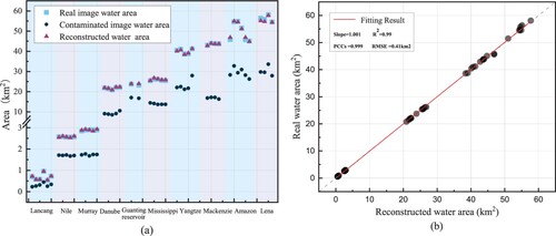
We compared the area of the 47 randomly chosen samples of real surface water, contaminated surface water, and rebuilt surface water in Figure 4a. The outcome showed that the recreated water area was considerably superior to the contaminated water region and closely resembled the actual water area. With a linear fitting of 1.001, a PCC of 0.999, and an RMSE of 0.41 km², the scatter diagram between the reconstructed water area and the actual water area shown in Figure 4b demonstrated a good correlation, high fidelity, and accuracy between them.

Figure 4. Overall accuracy evaluation results: (a) area comparison among the surface water reconstruction results, the contaminated water, and the real water, (b) scatter of the reconstructed water area and real water area.

4. Application results

4.1. Applications in type I water bodies

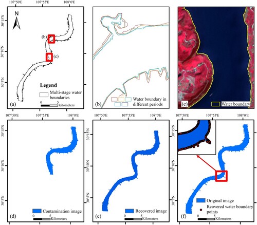
The Lancang River, Yangtze River, Amazon River, Lena River, and Guanting Reservoir were all found to be Type I water bodies in the sampled water bodies. These bodies of water showed clear seasonal variations in water level. Additionally, it was found that the water border sequence's position shift frequently exceeded three pixels.

Figure 5a to f show the Yangtze River reconstruction results. They show the water boundary error within a pixel (Figure 5a to c), the simulated contaminated image where the blue area was unaffected water (Figure 5d). The reconstructed water image (Figure 5e) is very similar to the original water image (Figure 5f). And in Figure 5f, the reconstructed water boundary points are also in close locations to the original water boundary. Additionally, the reconstructed water area (40.43 km²) has a relative error of only 0.7% compared with the real water area (40.12 km²).

Figure 5. Surface water reconstruction results of the Yangtze River: (a) construction results of the water boundary sequence; (b) details of the water boundary sequence; (c) superposition map of the image and its water boundary extraction results. The background image is Sentinel-2, and the band combination is B8 (near-infrared band), B4 (red band), and B3 (green band); (d) sample image is randomly cropped to simulate the contaminated image affected by clouds; (e) water image reconstructed with this method; (f) the original water image used for method testing and the superposition of the original water image and the reconstructed water boundary point.

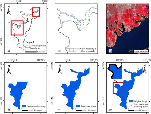
The surface water reconstruction results for Guanting Reservoir revealed that this algorithm has a high accuracy for large water bodies (Figure 6a-f). In Figure 6e and f, the shape and area of the reconstructed water and real water were similar, and the reconstructed boundary points were highly consistent with the real water boundary. The reconstructed water area and real water having a relative error of 0.7%, they were observed to be 23.71 and 23.87 km² respectively.

Figure 6. Surface water reconstruction results of the Guanting Reservoir: (a) construction results of the water boundary sequence; (b) details of the water boundary sequence; (c) superposition map of the image and its water boundary extraction results. The background image is Sentinel-2, and the band combination is B8 (near-infrared band), B4 (red band), and B3 (green band); (d) sample image is randomly cropped to simulate the contaminated image affected by clouds; (e) water image reconstructed with this method; (f) the original water image used for method testing and the superposition of the original water image and the reconstructed water boundary point.

The Lancang River, the Lena River, and the Amazon River's surface water reconstruction results, shown in Figures S2-S4, it was found that the reconstructed water borders were very compatible with the actual water boundary in the original images. Additionally, it was noted that the reconstructed water image's water areas and shapes were similar to those in the original water image.

4.2. Applications in type II water bodies

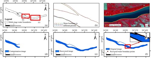
The Type II water bodies were found in the other five river section samples, which included the Nile River, Murray River, Mississippi River, Mackenzie River, and Danube River. They also had undetectable changes in water boundaries, where the change in water level was less than three pixels on the remote sensing images.

Figure 7's results from the surface water reconstruction for the Danube River show that the real and rebuilt waters have similar areas and shapes, and the boundary locations between the two are very consistent (Figure 7e and f). The measured values for the true water area and the rebuilt water area were 21.94 and 21.85 km², respectively, with a relative error of 0.4%. This finding suggests that this method can produce decent results in river stretches with big islands, with performance mostly dependent on the accuracy of the center line extraction.

Figure 7. Surface water reconstruction results for the Danube River: (a) construction results of the water boundary sequence; (b) details of the water boundary sequence; (c) superposition map of the image and its water boundary extraction results. The background image is Sentinel-2, and the band combination is B8 (near-infrared band), B4 (red band), and B3 (green band); (d) sample image is randomly cropped to simulate the contaminated image affected by clouds; (e) water image reconstructed with this method; (f) the original water image used for method testing and the superposition of the original water image and the reconstructed water boundary point.

The water extraction, sequential water boundary building, and surface water reconstruction results of the various river sections demonstrated good reliability and fidelity, as shown by the results for the Nile River, Murray River, Mississippi River, and Mackenzie River given in Figures S5–S8. The Nile reach was found to have the highest relative inaccuracy of water area (1.5%) among the other river portions. This is due to the observation that the water image was disrupted by the bridge across this portion of the Nile River. Due to the greater destruction of the main river center line caused by the removal of each center line's endpoint, the restored water area will be underestimated as a result.

4.3. Time-series surface water reconstruction applications

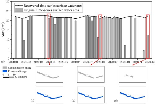
The entire time-series surface water construction application for the Lancang and Danube Rivers was chosen to demonstrate the algorithm's efficacy for the actual contaminated images. Images in these two research areas that had no water pixels were discarded. The images chosen either completely covered the research area or just concealed a very small land by cloud. In the Lancang River, a total of 29 images were collected in 2020; however, only 62% of these images were available due to cloud cover, 11 of the total images affected by cloud. In the Danube River, a total of 42 images were collected, with a 69% image availability rate. The lower image availability cause the challenge to directly detect surface water change characteristics using the original images.

The surface water of all cloud-contaminated images of the two rivers was retrieved using the surface water reconstruction algorithms suggested in section 2.2.3. The rebuilt results demonstrated all contaminated images were recovered and the precise surface water inundation boundaries (Figures 8 and 9). Additionally, the area of the missing water recovery had an effect on the water area's ongoing changing trend. For instance, a high water area on September 4, 2020, which was initially challenging to get using the original data sequence, was discovered by the recovered time-series surface water area curve of the Lancang River. Similarly, in Danube, the water area in this study section was stable at 21 km² all year-round, but great fluctuations were observed while using the original data sequence.

Figure 8. Original and recovered time-series surface water area of Lancang River, and the recovered results from real contamination images.

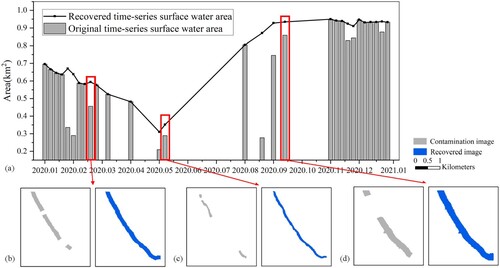
Figure 9. Original and recovered time-series surface water area of Danube River, and the recovered results from real contamination images.

With greater rainfall in the summer, the Lancang River region has a tropical and subtropical climate. In order to test the algorithm's effectiveness in places with cloudy and rainy weather, this region was selected for the time-series surface water reconstruction application. In the Lancang River application, combining the two water reconstruction algorithms, as was discussed in Section 5.1 of the discussion, maximizes the use of the images and addresses the problem of recovering the highest or lowest boundary water boundaries. For instance, the Type II of water body reconstruction method can be employed if higher and lower water border enclosures cannot be located. Compared to all water boundaries extracted from high-quality pictures, the water boundary of the Lancang River between May 2nd and May 7th, 2020, is lower. After that, we can decide to compute the distance relationship with the water border on April 2, 2020, and then constrict the water boundary to reassemble it. The strategy of expanding an entire border of adjacent dates can also be used to retrieve the highest water boundary. The quality standards for multi-stage water boundaries can be lowered with this reconstruction approach.

5. Discussion

5.1. Comparison with existing water mapping and reconstruction methods

The proposed method in this study exhibited several merits compared with recent water mapping or recovery methods (Pekel et al. 2016; Yao et al. 2019; Zhao and Gao 2018; Schwatke, Scherer, and Dettmering 2019). Firstly, our water extraction method based on adaptive thresholding to segment NDWI images did not require the collection of extensive training datasets such as the water extraction method of the Globe Surface Water (GSW) production (Pekel et al. 2016). In addition, we considered the degree of change in the water boundary, proposing a separate reconstruction algorithm. For the same river, we propose using the Type I method during a season with high water level change, and the Type II method during a season with low water level change. The combined use of these two types of methods can increase the availability of image data. For example, the Type II method's ability to calculate the distance relationship of the highest or lowest contaminated boundary with the reference boundary is sufficient to provide solutions to the problems encountered by Yao et al. (2019) in recovering the highest/lowest boundary water area. Furthermore, Yao et al. (2019) prioritized lake/reservoir areas over detailed inundation boundaries. The length of the river centerline can be used to calculate the average river width. However, determining the width of the river at a specific cross-section is difficult. The detailed inundation boundaries can help us calculate morphological parameters, river width, understand river changes more intuitively, and play an important role in river stability analysis and runoff estimation. Last but not least, Zhao and Gao (2018) used the GSW water occurrence image, Schwatke, Scherer, and Dettmering (2019) used Landsat and Sentinel-2 images to map their water occurrence image. A water boundary of water occurrence may not correspond to a realistic water shoreline and has fewer consistencies in adjacent periods due to uneven or insufficient no-cloud observations within the water body. In our study, there are enough images from Sentinel-2 to design multi-level water boundaries within a year, even if the quantity of no-cloud observations also impacts the quality of multi-stage water boundaries. Based on contraction and expansion with reference bounds, the reconstructed boundaries were more realistic.

5.2. Factors influencing the surface water reconstruction algorithm

5.2.1. Available reference remote sensing data

Based on the fact that the multi-stage water boundaries with sparse water boundary sequences show an elevation variation that is less linear. It will make it more difficult to fully explain changes in bank terrain, leading to a significant fluctuation in the value of k, which in turn affects how well the reconstruction turns out. It can be challenging to locate reference data to reconstruct the multi-stage water border in some regions with dense cloud cover and a lengthy rainy season because there are sometimes few photos available. Other satellite data, such as Sentinel-1 SAR data, can be used as a stand-in in this situation. This satellite sensor can function day and night and in almost any weather (Zeng et al. 2017; Bioresita et al. 2018), and can be used directly in the water extraction method. To build a comprehensive time-series water border, additional optical satellite remote sensing images with bands to generate NDWI index can also be employed directly as a source of additional information. Areas with significant swings in k values can also be treated independently if there aren't any more image data to encrypt the water boundaries.

5.2.2. Water boundary binary image transformation

The conversion of the water border into a binary picture was another crucial step in all the steps of the approach used in this study, and it had the potential to impact how accurately the reconstruction results were produced. Due to the use of the parallel capabilities of the map loop function in GEE in each computation of the rebuilt boundary point location (Safanelli et al. 2020). It was challenging to convert the raster by successively linking these boundary points to a tight graph during the loop since each water boundary point functioned independently and had no adjacent boundary points geographical information. This problem was solved by merging all lines that connect the boundary point with the corresponding center point in section 2.2.3. But the center line had fewer pixels than the boundary's, particularly on the outer circle of a river turn. While the edge pixels couldn't be produced without reconstructed point information. These circumstances did not frequently occur in this study, hence they had little impact on the reconstruction outcomes. The edge effect was noticeable for rivers that meandered with a lot of curves and bends. Hence, these rivers require the manual joining of the reconstructed boundary points to form a closed graph.

5.3. Limitation of the surface water reconstruction algorithm

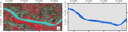
The surface water reconstruction algorithm described in this work can be used to the majority of rivers, lakes, and reservoirs, according to the robustness and verification analysis completed in this study. However, it had a number of drawbacks when applied to a body of water with intricate and mutable geometric features, such as the Yellow River sandbars created by flow transit and accumulation (Figure 10). This is due to the fact that sandbars’ shape, location, aggregation, and degree of fragmentation fluctuate drastically before and during the flood season (Li et al. 2022a). The production of the river center line was quite challenging in these locations due to the intricate interaction between the surface water and the surrounding terrain, which greatly influenced the outcomes of the reconstruction. Reclassification of sandbars as water bodies using the river's maximum boundary appears to be a viable solution. Sandbars in bodies of water, for example, can be removed by filling isolated islands, whereas sandbars connected to the bank can be manually connected to the river boundary disconnection point. However, this would significantly reduce the program's automation.

Figure 10. River surface water fragmentation caused by sandbars in the Yellow River. (a) Sentinel-2 image, band combination: B8 (near-infrared band), B4 (red band), B3 (green band), (b) water extraction results.

Our water reconstruction was based on linear interpolation between the water extent at the nearest isobath, as assumed in the methods section. However, nonlinear changes in bank topography will introduce errors. The magnitude of the error will be determined by the condition of the multi-stage water boundaries. The nonlinear characteristics of the river bank will be reflected by them when the number of water boundaries is large enough and the distribution is uniform enough. Nonlinearity between neighboring multi-stage boundaries will be reduced. The multi-stage water boundaries are spaced closer together where the slope is steep and farther apart where the slope is gentle. The nonlinearity between the nearest multi-stage boundaries will be less accurate if sparse water boundaries are used for reconstruction.

6. Conclusions

A surface water reconstruction method based on the spatial distance relationship of multi-stage water boundaries was proposed in this paper. The application of this method on 47 sample images from ten large rivers around the world in 2020 demonstrates that it is a fine surface water reconstruction method with very high accuracy. The reconstructed and real water areas also demonstrated a high level of consistency and coincidence, with PCCs of 0.99, RMSEs of 0.41 km², and a relative error range of less than 5%. Furthermore, time-series surface water reconstruction has been shown to be an effective method for restoring contaminated pixels caused by clouds and cloud shadows, improving image availability, and obtaining high temporal resolution surface water datasets. The GEE-implemented tools based on this algorithm have a lot of potential for large-scale applications.

When we don't have the available images and don't want to sacrifice the temporal resolution of the satellite images, reconstructing the contaminated water pixels may be a better option. Although the current satellite temporal resolution limits this method's ability to satisfy a daily or single-day frequency surface water data requirement, it does have the capability of integrating most synthetic aperture radar and optical satellite data to construct time-series water boundary sequences, which will improve the accuracy of surface water reconstruction and higher-frequency datasets. In the future, we plan to use this method to create high-frequency surface water data products in scenarios requiring high temporal resolution, such as bridging the large monitoring frequency gap between existing remote sensing runoff estimation and measured runoff. Furthermore, elevation data from the radar altimeter will be used to create an elevation index for water boundaries, which will aid us in the automatic selection of reference water boundaries based on the elevation relationship between them.

Acknowledgements

We thank the anonymous reviewers for their constructive comments on this manuscript.

Data availability statement (DAS)

The remote sensing images are available from the GEE data repository (https://developers.google.com/earth-engine/datasets/). The Global River Widths from Landsat datasets are downloaded from https://doi.org/10.5281/zenodo.1297434.

Disclosure statement

No potential conflict of interest was reported by the author(s).

Additional information

Funding

The research was funded by the National Natural Science Foundation of China [grant no 42171283], the Major Science and Technology Projects of Qinghai Province [grant no 2021-SF-A6], the Second Tibetan Plateau Scientific Expedition and Research Program (STEP) [grant number 2019QZKK0202], and Strategic Priority Research Program of the Chinese Academy of Sciences [grant number XDA19090120].

References

- Allen, George H., and Tamlin M. Pavelsky. 2015. “Patterns of River Width and Surface Area Revealed by the Satellite-Derived North American River Width Data Set.” Geophysical Research Letters 42 (2): 395–402. doi:10.1002/2014GL062764.
- Allen, George H., and Tamlin M. Pavelsky. 2018. “Global Extent of Rivers and Streams.” Science 361 (6402): 585–588. doi:10.1126/science.aat0636.
- Bao, Linan, Xiaolei Lv, and Jingchuan Yao. 2021. “Water Extraction in SAR Images Using Features Analysis and Dual-Threshold Graph Cut Model.” Remote Sensing 13 (17), doi:10.3390/rs13173465.
- Becker, Willyan Ronaldo, Thiago Berticelli Ló, Jerry Adriani Johann, and Erivelto Mercante. 2021. “Statistical Features for Land Use and Land Cover Classification in Google Earth Engine.” Remote Sensing Applications: Society and Environment 21: 100459. doi:https://doi.org/10.1016/j.rsase.2020.100459.
- Bhangale, Ujwala, Swapnil More, Tanishq Shaikh, Suchitra Patil, and Nilkamal More. 2020. “Analysis of Surface Water Resources Using Sentinel-2 Imagery.” Procedia Computer Science 171: 2645–2654. doi:10.1016/j.procs.2020.04.287.
- Bioresita, Filsa, Anne Puissant, André Stumpf, and Jean-Philippe Malet. 2018. “A Method for Automatic and Rapid Mapping of Water Surfaces from Sentinel-1 Imagery.” Remote Sensing 10 (2): 217. doi:https://doi.org/10.3390/rs10020217.
- Bonafilia, D., B. Tellman, T. Anderson, and E. Issenberg. 2020. “Sen1Floods11: A Georeferenced Dataset to Train and Test Deep Learning Flood Algorithms for Sentinel-1.” Paper presented at the 2020 IEEE/CVF Conference on Computer Vision and Pattern Recognition Workshops (CVPRW), 14-19 June 2020. doi:10.1109/CVPRW50498.2020.00113.
- Boothroyd, Richard J., Richard D. Williams, Trevor B. Hoey, Brian Barrett, and Octria A. Prasojo. 2021. “Applications of Google Earth Engine in Fluvial Geomorphology for Detecting River Channel Change.” WIRES Water 8 (1): e21496. doi:10.1002/wat2.1496.
- Canny, John. 1986. “A Computational Approach to Edge Detection.” IEEE Transactions on Pattern Analysis and Machine Intelligence 6: 679–698. doi:10.1109/TPAMI.1986.4767851.
- Cheng, G., X. Xie, J. Han, L. Guo, and G. S. Xia. 2020. “Remote Sensing Image Scene Classification Meets Deep Learning: Challenges, Methods, Benchmarks, and Opportunities.” IEEE Journal of Selected Topics in Applied Earth Observations and Remote Sensing 13: 3735–3756. doi:10.1109/JSTARS.2020.3005403.
- Chini, M., R. Hostache, L. Giustarini, and P. Matgen. 2017. “A Hierarchical Split-Based Approach for Parametric Thresholding of SAR Images: Flood Inundation as a Test Case.” IEEE Transactions on Geoscience and Remote Sensing 55 (12): 6975–6988. doi:10.1109/TGRS.2017.2737664.
- DeVries, Ben, Chengquan Huang, John Armston, Wenli Huang, John W. Jones, and Megan W. Lang. 2020. “Rapid and robust monitoring of flood events using Sentinel-1 and Landsat data on the Google Earth Engine.” Remote Sensing of Environment 240: 111664. doi:10.1016/j.rse.2020.111664.
- Donchyts, Gennadii, Fedor Baart, Hessel Winsemius, Noel Gorelick, Jaap Kwadijk, and Nick van de Giesen. 2016a. “Earth's Surface Water Change Over the Past 30 Years.” Nature Climate Change 6 (9): 810–813. doi:10.1038/nclimate3111.
- Donchyts, Gennadii, Jaap Schellekens, Hessel Winsemius, Elmar Eisemann, and Nick Van de Giesen. 2016b. “A 30 m Resolution Surface Water Mask Including Estimation of Positional and Thematic Differences Using Landsat 8, SRTM and OpenStreetMap: A Case Study in the Murray-Darling Basin, Australia.” Remote Sensing 8 (5), doi:10.3390/rs8050386.
- Du, Yun, Yihang Zhang, Feng Ling, Qunming Wang, Wenbo Li, and Xiaodong Li. 2016. “Water Bodies’ Mapping from Sentinel-2 Imagery with Modified Normalized Difference Water Index at 10-m Spatial Resolution Produced by Sharpening the SWIR Band.” Remote Sensing 8 (4), doi:10.3390/rs8040354.
- Feng, Dongmei, Colin J Gleason, Peirong Lin, Xiao Yang, Ming Pan, and Yuta Ishitsuka. 2021. “Anomalous Collapses of Nares Strait ice Arches Leads to Enhanced Export of Arctic sea ice.” Nature Communications 12 (1): 1–9. doi:10.1038/s41467-020-20314-w.
- Ficklin, Darren L., John T. Abatzoglou, and Kimberly A. Novick. 2019. “A New Perspective on Terrestrial Hydrologic Intensity That Incorporates Atmospheric Water Demand.” Geophysical Research Letters 46 (14): 8114–8124. doi:10.1029/2019GL084015.
- Gao, Huilin, Charon Birkett, and Dennis P. Lettenmaier. 2012. “Global Monitoring of Large Reservoir Storage from Satellite Remote Sensing.” Water Resources Research 48 (9), doi:10.1029/2012WR012063.
- Gleason, Colin J, and Michael T Durand. 2020. “Remote Sensing of River Discharge: A Review and a Framing for the Discipline.” Remote Sensing 12 (7): 1107. doi:10.3390/rs12071107.
- Gorelick, Noel, Matt Hancher, Mike Dixon, Simon Ilyushchenko, David Thau, and Rebecca Moore. 2017. “Google Earth Engine: Planetary-Scale Geospatial Analysis for Everyone.” Remote Sensing of Environment 202: 18–27. doi:10.1016/j.rse.2017.06.031.
- Gu, Xihui, Qiang Zhang, Jianfeng Li, Deliang Chen, Vijay P. Singh, Yongqiang Zhang, Jianyu Liu, Zexi Shen, and Huiqian Yu. 2020. “Impacts of Anthropogenic Warming and Uneven Regional Socio-Economic Development on Global River Flood Risk.” Journal of Hydrology 590: 125262. doi:10.1016/j.jhydrol.2020.125262.
- Heimhuber, V., M. G. Tulbure, and M. Broich. 2016. “Modeling 25 Years of Spatio-Temporal Surface Water and Inundation Dynamics on Large River Basin Scale Using Time Series of Earth Observation Data.” Hydrology and Earth System Sciences 20 (6): 2227–2250. doi:10.5194/hess-20-2227-2016.
- Huang, Huabing, Yanlei Chen, Nicholas Clinton, Jie Wang, Xiaoyi Wang, Caixia Liu, Peng Gong, et al. 2017. “Mapping Major Land Cover Dynamics in Beijing Using all Landsat Images in Google Earth Engine.” Remote Sensing of Environment 202: 166–176. doi:10.1016/j.rse.2017.02.021.
- Huang, Chang, Yun Chen, Shiqiang Zhang, and Jianping Wu. 2018. “Detecting, Extracting, and Monitoring Surface Water from Space Using Optical Sensors: A Review.” Reviews of Geophysics 56 (2): 333–360. doi:10.1029/2018RG000598.
- Huang, Xingying, and Daniel L. Swain. 2022. “Climate Change is Increasing the Risk of a California Megaflood.” Science Advances 8 (32), doi:10.1126/sciadv.abq0995.
- Huang, Xin, Cong Xie, Xing Fang, and Liangpei Zhang. 2015. “Combining Pixel- and Object-Based Machine Learning for Identification of Water-Body Types from Urban High-Resolution Remote-Sensing Imagery.” IEEE Journal of Selected Topics in Applied Earth Observations and Remote Sensing 8 (5): 2097–2110. doi:10.1109/JSTARS.2015.2420713.
- Huntington, Thomas G., Peter K. Weiskel, David M. Wolock, and Gregory J. McCabe. 2018. “A new Indicator Framework for Quantifying the Intensity of the Terrestrial Water Cycle.” Journal of Hydrology 559: 361–372. doi:https://doi.org/10.1016/j.jhydrol.2018.02.048.
- Isikdogan, Furkan, Alan C Bovik, and Paola Passalacqua. 2017. “Surface Water Mapping by Deep Learning.” IEEE Journal of Selected Topics in Applied Earth Observations and Remote Sensing 10 (11): 4909–4918. doi:10.1109/JSTARS.2017.2735443.
- Jakovljević, Gordana, and Miro Govedarica. 2019. “Water Body Extraction and Flood Risk Assessment Using Lidar and Open Data.” Climate Change Adaptation in Eastern Europe: Managing Risks and Building Resilience to Climate Change, 93–111. doi:10.1007/978-3-030-03383-5_7.
- Jiang, Zijie, Weiguo Jiang, Ziyan Ling, Xiaoya Wang, Kaifeng Peng, and Chunlin Wang. 2021. “Surface Water Extraction and Dynamic Analysis of Baiyangdian Lake Based on the Google Earth Engine Platform Using Sentinel-1 for Reporting SDG 6.6.1 Indicators.” Water 13 (2), doi:10.3390/w13020138.
- John, E. Ball, T. Anderson Derek, and S. R. Chan Chee Seng. 2017. “Comprehensive Survey of Deep Learning in Remote Sensing: Theories, Tools, and Challenges for the Community.” Journal of Applied Remote Sensing 11 (4): 042609. doi:10.1117/1.JRS.11.042609.
- Kebede, Mulugeta Genanu, Lei Wang, Xiuping Li, and Zhidan Hu. 2020. “Remote Sensing-Based River Discharge Estimation for a Small River Flowing Over the High Mountain Regions of the Tibetan Plateau.” International Journal of Remote Sensing 41 (9): 3322–3345. doi:10.1080/01431161.2019.1701213.
- Khandelwal, Ankush, Anuj Karpatne, Miriam E. Marlier, Jongyoun Kim, Dennis P. Lettenmaier, and Vipin Kumar. 2017. “An Approach for Global Monitoring of Surface Water Extent Variations in Reservoirs Using MODIS Data.” Remote Sensing of Environment 202: 113–128. doi:10.1016/j.rse.2017.05.039.
- Li, Peng, Shenliang Chen, Lanqing Liu, and Chenyu Zhang. 2022a. “Response of Sandbar and Estuarine Morphology at the Tail end of the Yellow River to Water and Sediment Changes.” Journal of Sediment Research, 1–8. doi:10.16239/j.cnki.0468-155x.2022.02.009.
- Li, Aimin, Meng Fan, Guangduo Qin, Youcheng Xu, and Hailong Wang. 2021. “Comparative Analysis of Machine Learning Algorithms in Automatic Identification and Extraction of Water Boundaries.” Applied Sciences 11 (21): 10062. doi:10.3390/app112110062.
- Li, Yang, Zhenguo Niu, Zeyu Xu, and Xin Yan. 2020b. “Construction of High Spatial-Temporal Water Body Dataset in China Based on Sentinel-1 Archives and GEE.” Remote Sensing 12 (15): 2413. doi:10.3390/rs12152413.
- Li, Zhiwei, Huanfeng Shen, Qihao Weng, Yuzhuo Zhang, Peng Dou, and Liangpei Zhang. 2022. “Cloud and Cloud Shadow Detection for Optical Satellite Imagery: Features, Algorithms, Validation, and Prospects.” ISPRS Journal of Photogrammetry and Remote Sensing 188: 89–108. doi:10.1016/j.isprsjprs.2022.03.020.
- Li, Junli, and Yongwei Sheng. 2012. “An Automated Scheme for Glacial Lake Dynamics Mapping Using Landsat Imagery and Digital Elevation Models: A Case Study in the Himalayas.” International Journal of Remote Sensing 33: 5194–5213. doi:10.1080/01431161.2012.657370.
- Li, Sanmei, Donglian Sun, Mitchell Goldberg, and Anthony Stefanidis. 2013. “Derivation of 30-m-Resolution Water Maps from TERRA/MODIS and SRTM.” Remote Sensing of Environment 134: 417–430. doi:10.1016/j.rse.2013.03.015.
- Liu, Kai, Chunqiao Song, Jida Wang, Linghong Ke, Yunqiang Zhu, Jingying Zhu, Ronghua Ma, and Zhu Luo. 2020. “Remote Sensing-Based Modeling of the Bathymetry and Water Storage for Channel-Type Reservoirs Worldwide.” Water Resources Research 56 (11): e2020WR027147. doi:10.1029/2020WR027147.
- López-Caloca, Alejandra A., Felipe Omar Tapia-Silva, Fernando López, Henao Pilar, Aymara O. Ramírez González, and Guadalupep Rivera. 2020. “Analyzing Short Term Spatial and Temporal Dynamics of Water Presence at a Basin-Scale in Mexico Using SAR Data.” GIScience & Remote Sensing 57 (7): 985–1004. doi:10.1080/15481603.2020.1840106.
- Lu, Shanlong, Li Jia, Lei Zhang, Yongping Wei, Muhammad Hasan Ali Baig, Zhaokun Zhai, Jihua Meng, Xiaosong Li, and Guifang Zhang. 2017. “Lake Water Surface Mapping in the Tibetan Plateau Using the MODIS MOD09Q1 Product.” Remote Sensing Letters 8 (3): 224–233. doi:10.1080/2150704X.2016.1260178.
- Martinis, Sandro, Claudia Kuenzer, Anna Wendleder, Juliane Huth, André Twele, Achim Roth, and Stefan Dech. 2015. “Comparing Four Operational SAR-Based Water and Flood Detection Approaches.” International Journal of Remote Sensing 36 (13): 3519–3543. doi:10.1080/01431161.2015.1060647.
- Matgen, P., G. Schumann, J. B. Henry, L. Hoffmann, and L. Pfister. 2007. “Integration of SAR-Derived River Inundation Areas, High-Precision Topographic Data and a River Flow Model Toward Near Real-Time Flood Management.” International Journal of Applied Earth Observation and Geoinformation 9 (3): 247–263. doi:10.1016/j.jag.2006.03.003.
- Maxwell, Aaron E., Timothy A. Warner, and Fang Fang. 2018. “Implementation of Machine-Learning Classification in Remote Sensing: An Applied Review.” International Journal of Remote Sensing 39 (9): 2784–817. doi:10.1080/01431161.2018.1433343.
- McFeeters, S. K. 1996. “The use of the Normalized Difference Water Index (NDWI) in the Delineation of Open Water Features.” International Journal of Remote Sensing 17 (7): 1425–1432. doi:10.1080/01431169608948714.
- Mengen, David, Marco Ottinger, Patrick Leinenkugel, and Lars Ribbe. 2020. “Modeling River Discharge Using Automated River Width Measurements Derived from Sentinel-1 Time Series.” Remote Sensing 12 (19): 3236. doi:10.3390/rs12193236.
- Misra, Gourav, Fiona Cawkwell, and Astrid Wingler. 2020. “Status of Phenological Research Using Sentinel-2 Data: A Review.” Remote Sensing 12 (17), doi:10.3390/rs12172760.
- Mou, Xiaoli, He Li, Chong Huang, Qingsheng Liu, and Gaohuan Liu. 2021. “Application Progress of Google Earth Engine in Land use and Land Cover Remote Sensing Information Extraction.” Remote Sensing for Land & Resources 33 (2): 1–10. doi:10.6046/gtzyyg.2020189.
- Ni, Rongguang, Jinyan Tian, Xiaojuan Li, Dameng Yin, Jiwei Li, Huili Gong, Jie Zhang, Lin Zhu, and Dongli Wu. 2021. “An Enhanced Pixel-Based Phenological Feature for Accurate Paddy Rice Mapping with Sentinel-2 Imagery in Google Earth Engine.” ISPRS Journal of Photogrammetry and Remote Sensing 178: 282–296. doi:doi:10.1016/j.isprsjprs.2021.06.018.
- Ogilvie, Andrew, Gilles Belaud, Sylvain Massuel, Mark Mulligan, Patrick Le Goulven, Pierre-Olivier Malaterre, and Roger Calvez. 2018. “Combining Landsat Observations with Hydrological Modelling for Improved Surface Water Monitoring of Small Lakes.” Journal of Hydrology 566: 109–121. doi:10.1016/j.jhydrol.2018.08.076.
- Otsu, Nobuyuki. 1979. “A Threshold Selection Method from Gray-Level Histograms.” IEEE Transactions on Systems, man, and Cybernetics 9 (1): 62–66. doi:10.1109/TSMC.1979.4310076.
- Pekel, Jean-François, Andrew Cottam, Noel Gorelick, and Alan S. Belward. 2016. “High-resolution Mapping of Global Surface Water and its Long-Term Changes.” Nature 540 (7633): 418–422. doi:10.1038/nature20584.
- Rwanga, Sophia S., and J. M. Ndambuki. 2017. “Accuracy Assessment of Land Use/Land Cover Classification Using Remote Sensing and GIS.” International Journal of Geosciences 08 (04): 12. doi:10.4236/ijg.2017.84033.
- Safanelli, José Lucas, Raul Roberto Poppiel, Luis Fernando Chimelo Ruiz, Benito Roberto Bonfatti, Fellipe Alcantara de Oliveira Mello, Rodnei Rizzo, and José A. M. Demattê. 2020. “Terrain Analysis in Google Earth Engine: A Method Adapted for High-Performance Global-Scale Analysis.” ISPRS International Journal of Geo-Information 9 (6): 400. doi:doi:10.3390/ijgi9060400.
- Schiermeier, Quirin. 2011. “Increased Flood Risk Linked to Global Warming.” Nature 470 (7334): 316. doi:10.1038/470316a.
- Schmitt, Michael, Lloyd Hughes, Chunping Qiu, and Xiao Zhu. 2019. “SEN12MS - A Curated Dataset of Georeferenced Multi-Spectral Sentinel-1/2 Imagery for Deep Learning and Data Fusion.” Vol. IV-2/W7. doi:10.5194/isprs-annals-IV-2-W7-153-2019.
- Schwatke, Christian, Daniel Scherer, and Denise Dettmering. 2019. “Automated Extraction of Consistent Time-Variable Water Surfaces of Lakes and Reservoirs Based on Landsat and Sentinel-2.” Remote Sensing 11 (9), doi:10.3390/rs11091010.
- Soulard, Christopher E., Eric K. Waller, Jessica J. Walker, Roy E. Petrakis, and Britt W. Smith. 2022. “DSWEmod — The Production of High-Frequency Surface Water Map Composites from Daily MODIS Images.” JAWRA Journal of the American Water Resources Association 58 (2): 248–268. doi:10.1111/1752-1688.12996.
- Tamiminia, Haifa, Bahram Salehi, Masoud Mahdianpari, Lindi Quackenbush, Sarina Adeli, and Brian Brisco. 2020. “Google Earth Engine for geo-big Data Applications: A Meta-Analysis and Systematic Review.” ISPRS Journal of Photogrammetry and Remote Sensing 164: 152–170. doi:10.1016/j.isprsjprs.2020.04.001.
- Wang, Y., M. Liao, G. Sun, and J. Gong. 2005. “Analysis of the Water Volume, Length, Total Area and Inundated Area of the Three Gorges Reservoir, China Using the SRTM DEM Data.” International Journal of Remote Sensing 26 (18): 4001–4012. doi:10.1080/01431160500176788.
- Wang, Jida, Chunqiao Song, John T Reager, Fangfang Yao, James S Famiglietti, Yongwei Sheng, Glen M MacDonald, Fanny Brun, Hannes Müller Schmied, and Richard A Marston. 2018. “Recent Global Decline in Endorheic Basin Water Storages.” Nature Geoscience 11 (12): 926–932. doi:doi:10.1038/s41561-018-0265-7.
- Yang, Xiao, Tamlin M. Pavelsky, George H. Allen, and Gennadii Donchyts. 2020. “RivWidthCloud: An Automated Google Earth Engine Algorithm for River Width Extraction from Remotely Sensed Imagery.” IEEE Geoscience and Remote Sensing Letters 17 (2): 217–221. doi:10.1109/LGRS.2019.2920225.
- Yao, Fangfang, Jida Wang, Chao Wang, and Jean-François Crétaux. 2019. “Constructing Long-Term High-Frequency Time Series of Global Lake and Reservoir Areas Using Landsat Imagery.” Remote Sensing of Environment 232: 111210. doi:10.1016/j.rse.2019.111210.
- Yuan, Qiangqiang, Huanfeng Shen, Tongwen Li, Zhiwei Li, Shuwen Li, Yun Jiang, Hongzhang Xu, Weiwei Tan, Qianqian Yang, and Jiwen Wang. 2020. “Deep Learning in Environmental Remote Sensing: Achievements and Challenges.” Remote Sensing of Environment 241: 111716. doi:10.1016/j.rse.2020.111716.
- Zeng, Lingfang, Michael Schmitt, Lin Li, and Xiao Xiang Zhu. 2017. “Analysing Changes of the Poyang Lake Water Area Using Sentinel-1 Synthetic Aperture Radar Imagery.” International Journal of Remote Sensing 38 (23): 7041–7069. doi:10.1080/01431161.2017.1370151.
- Zhang, Yuanchong, William B. Rossow, Andrew A. Lacis, Valdar Oinas, and Michael I. Mishchenko. 2004. “Calculation of radiative fluxes from the surface to top of atmosphere based on ISCCP and other global data sets: Refinements of the radiative transfer model and the input data.” Journal of Geophysical Research: Atmospheres 109 (D19), doi:10.1029/2003JD004457.
- Zhao, Gang, and Huilin Gao. 2018. “Automatic Correction of Contaminated Images for Assessment of Reservoir Surface Area Dynamics.” Geophysical Research Letters 45 (12): 6092–6099. doi:10.1029/2018GL078343.