A comparison of three surface roughness characterization techniques: photogrammetry, pin profiler, and smartphone-based LiDAR

ABSTRACT

Surface roughness plays an important role in microwave remote sensing. In the agricultural domain, surface roughness is crucial for soil moisture retrieval methods that use electromagnetic surface scattering or microwave radiative transfer models. Therefore, improved characterization of Soil Surface Roughness (SSR) is of considerable importance. In this study, three approaches, including a standard pin profiler, a LiDAR point cloud generated from an iPhone 12 Pro, and a Structure from Motion (SfM) photogrammetric point cloud, were applied over 24 surface profiles with different roughness variations to measure surface roughness. The objective of this study was to evaluate the capability of smartphone-based LiDAR technology to measure surface roughness parameters and compare the results of this technique with the more common approaches. Results showed that the iPhone LiDAR technology, when point cloud data is captured in a fine-resolution mode, has a significant correlation with SfM photogrammetry (R²= 0.70) and a relatively close agreement with pin profiler (R²= 0.60). However, this accuracy tends to be greater for random surfaces and rough profiles with row structure orientations. The results of this study confirm that smartphone-based LiDAR can be used as a cost-effective, fast, and time-efficient alternative tool for measuring surface roughness, especially for rough, wide, and inaccessible areas.

KEYWORDS:

• LiDAR
• surface roughness
• structure from motion
• iPhone
• pin profiler

1. Introduction

The characterization of soil surface roughness (SSR) plays an important role in providing relevant information for microwave remote sensing monitoring and modelling. Inversion methods for soil moisture estimation, using active and passive microwave remote sensing measurements, are dependent on SSR data that must be known or derived in retrieval models. In these models, microwave energy, received by active and passive sensors, is used for soil moisture retrieval. However, microwave signals are highly affected by vegetation, soil moisture, and SSR (Das and Paul 2015). Sometimes, surface roughness has been reported to have a greater impact than other factors (Bryant et al. 2007), particularly in areas with bare soils. Therefore, it is critical to obtain a reliable assessment of SSR for different microwave remote sensing retrieval models such as emission (passive) and backscattering (active) models for soil moisture estimation. SSR is commonly described by root mean squared height (RMSH), which is defined as the standard deviation of surface elevation (Trudel et al. 2010). The correlation length is another roughness parameter and is identified as the maximum distance over which the correlation exists between profile surface heights (Gupta and Jangid 2011).

Agricultural SSR can be measured using two groups of methods, including contact and non-contact techniques. The most common contact technique to measure the parameters of SSR is the use of a pin profiler or a mesh board (Hajnsek, Pottier, and Cloude 2003; Le Morvan et al. 2008; Merzouki, McNairn, and Pacheco 2011; McNairn et al. 2012; Zheng et al. 2019). This technique is simple to set up in the field. Moreover, it has the capability of joining 1-m profiles to create a longer profile (Trudel et al. 2010). However, several limitations are associated with the application of a pin profiler in the field. The main disadvantage of the method is that the pins can alter the surface under observation (Jester and Klik 2005; Moreno et al. 2008; Landy et al. 2015). Additionally, data collection and processing are time-consuming (Chabot et al. 2018; Gharechelou, Tateishi, and Johnson 2018) and labour intensive to obtain in the field (Turner et al. 2014). Moreover, it is difficult to use this method across rough terrains or large areas, particularly in the fields with row soil structure created by cultivation (Blaes and Defourny 2008).

On the other hand, non-contact, or remote sensing-based techniques, are able to measure SSR in a wide-multidirectional area without disturbing the surfaces under observation. They are also applicable for remote and inaccessible locations. Common techniques for understanding roughness can be divided into two sets of approaches that either make an estimate of roughness through electromagnetic scattering models or physically measure the roughness by generating a 3D surface model. The electromagnetic scattering models typically use surface roughness parameters as input parameters. However, because of the lack of surface roughness measurements, several studies use electromagnetic scattering models for SSR inversion to compensate the lack of measurements (see for example Oh 2004; Kim et al. 2012; King et al. 2018). There are challenges associated with the application of these models. Primarily, the sensitivity of radar signals to SSR is more significant for low roughness levels (i.e. roughness approximately less than 1.5 cm in C-band) (Baghdadi, Holah, and Zribi 2006); therefore, the utilization of inversion models seems to be more relevant for smoother agricultural surfaces and not practical for rough fields (Davidson et al. 2000). Furthermore, in electromagnetic scattering models, surfaces have usually been considered as stationary, single scale and randomly rough surfaces (Fernandez Diaz et al. 2010), which may not be a realistic way of representing natural agricultural fields (Alijani et al. 2021).

Laser scanning technologies, terrestrial laser-scanning (TLS) and airborne laser-scanning (ALS), are among the most important techniques that use LiDAR technology for generating 3D surface models. These techniques provide fine-resolution data at a wide range of scales, ranging from kilometres for ALS (Hollaus et al. 2011) to a few metres for TLS (Landy et al. 2015). However, data acquisition by large-scale airborne laser scanners is very expensive. Since this technology uses third-party organizations and advanced flight planning, ALS data is generally not available to many researchers, particularity at the time scales needed in many applications. In contrast, TLS can provide higher temporal frequency data acquisition, with high spatial resolution, and can be utilized at any time by users. However, they are still expensive, and their utilization might not be applicable for everyone. Other disadvantages of TLS can be referred to: issues of shadowing, which refers to the non-detection of areas due to the shadow effect (Seidel and Ammer 2014); miscalculation of off-terrain objects (Roberts, Lindsay, and Berg 2019); and processing times for large high-resolution datasets (Rychkov, Brasington, and Vericat 2012). Moreover, like pin profiler, TLSs are somewhat limited when used in rough terrain (Luetzenburg, Kroon, and Bjørk 2021). In the past few decades, the drone-based technology had also a growing use for LiDAR data collection. The potential applications of drones significantly reduce the cost compared with ALS, while increase the spatial extent of scanning, compared with TLS (Kellner et al. 2019). However, they are not still affordable for every user and cannot be readily implemented as a measuring equipment in the field. In this case, the emergence of hand-held laser scanners with the ability to overcome the above limitations can open new doors for geoscience studies.

Smartphones and tablets have recently been released with built-in LiDAR sensors, e.g. the Apple iPad and iPhone Pro. The iPhone 12 Pro, released in October 2020, was the first smartphone equipped with a native LiDAR scanner. This technology enables capturing 3D scenes directly in the field, which is a potential paradigm shift in digital field data acquisition (Tavani et al. 2022) and the integration of LiDAR into a personal device generated high interest among professional users and consumers. Moreover, its availability has drawn the attention of app developers to develop 3D scanning apps, such as 3D scanner, Polycam and Pix4DCatch (Teppati Losè et al. 2022). Given the greater versatility and usability of smartphones and tablets in the field, this technology allows for faster monitoring of objects and easier access to data. Such capabilities provide opportunities to make research more repeatable and transparent and to make open access and low-cost geospatial data more accessible to the public. The ability of smartphone-based LiDAR has been evaluated in different applications, such as the 3D survey of rocks and cliffs for geological purposes (Luetzenburg, Kroon, and Bjørk 2021), monitoring snow depth changes (King, Kelly, and Fletcher 2022), forestry (Tatsumi,Yamaguchi, and Furuya 2021), and human body measurements (Mikalai et al. 2022). However, the capability of smartphone-based LiDAR sensors for surface roughness data collection must be evaluated for practical scientific purposes.

In addition to smartphone-based LiDAR technology, structure from motion (SfM) photogrammetry is another technique for generating fine-resolution surface reconstructions. Compared to high-cost laser scanners, this technique uses relatively low-cost photographic data, often captured using standard camera equipment. The SfM photogrammetry operates in the same way as stereoscopic photogrammetry, in which a 3D structure can be generated from a series of overlapping images (Westoby et al. 2012). This technique has been used recently for surface roughness characterization within agricultural fields and been compared against the fine-resolution TLS approach to evaluate its capability to measure roughness (Martinez-Agirre, Álvarez-Mozos, and Giménez 2016). Moreover, SfM photogrammetry has been evaluated in other applications, such as joint roughness profiling (Saricam and Ozturk 2022), rock discontinuities (Poropat 2009; Sturzenegger and Stead 2009; Kong et al. 2021), sediment transport (Zimmerman and Miller 2021; Dai et al. 2022), and forestry (Sakai et al. 2021; Gao and Kan 2022). The capability of the photogrammetry approach for surface roughness characterization was tested against pin profiler and laser scanner techniques by Jester and Klik (2005). They demonstrated that data acquisition using photogrammetry was faster compared to laser scanners and pin profilers. However, data processing takes the least time using a pin profiler, followed by a laser scanner and the most time-consuming using photogrammetry. In terms of uncertainty, laser scanners are more precise than photogrammetry and pin profilers because they can produce a far more detailed surface characterization. Rodríguez-Caballero et al. (2012) stated that photogrammetry and laser scanning are usually more accurate than using a pin profiler but laborious and time-consuming because they require considerable data processing. However, Vinci et al. (2020) reported that photogrammetry had lower-cost and speed advantages over laser scanners. In another study by Tao et al. (2017), the accuracy required for microwave inversion of surface roughness parameters obtained from photogrammetry and pin profilers was tested. Their results showed that this accuracy can be effectively improved by using photogrammetry and this technique can meet the requirements of roughness parameter inversion. Finally, in a study by Lavoie et al. (2006) that characterized SSR using a LiDAR scanner, photogrammetry and a pin profiler, they concluded that the pin profiler was the cheapest, fastest and easiest way to measure surface roughness. However, they showed that a laser scanner and photogrammetry can provide a picture of the target surface instead of a profile like the pin profiler, and this allows the user to make profiles everywhere on the surface and to use any kind of statistical surface analysis. Regardless of the many studies for SSR characterization, the ability of smartphone-based LiDAR for surface roughness characterization compared to pin profiler and SfM photogrammetry has not been evaluated for different roughness profiles.

Therefore, the overall goal of this study is to analyze the capability of smartphone-based LiDAR technology for the characterization of surface roughness parameters. The specific objectives of this study are to:

1. Characterize surface roughness of a complex surface using a pin profiler, smartphone-based LiDAR, and SfM photogrammetry in the laboratory.

2. Validate the accuracy of SfM photogrammetry and smartphone-based LiDAR technology using pin profiler measurements.

3. Compare the results of surface roughness characterization by pin profiler, SfM photogrammetry, and smartphone-based LiDAR.

2. Material and methods

2.1. Site description

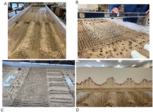
A laboratory experiment was conducted, where 24 different roughness elements were constructed using moistened sand in a hydrological flume (length: 610 cm, width: 125 cm, height: 23 cm). The setup allows to remove the external environmental factors and human impacts on the surfaces. The construction of surfaces was designed, with different approaches, in order to develop both random and patterned roughness conditions that may be associated with agricultural field surfaces with various tillage depth (Figure 1(a)). Each surface roughness element was marked and numbered using tape on the edge of the flume to have a consistent measurement of each roughness.

Figure 1. Steps for surface roughness data collection: Image (a) shows 24 various surface roughness profiles across the flume; Image (b) indicates the method of scanning profiles using iPhone LiDAR; Image (c) shows the locations of paper targets on the profile surfaces as well as on the edges of the flume for the SfM approach; and Image (d) shows the wooden pin profiler measuring roughness.

2.2. Surface roughness data collection

To avoid disturbing the surface with the compression effect caused by the pin profiler, surface roughness measurements were first conducted by the ‘3d Scanner App’ installed on iPhone 12 Pro and then the imagery data used for the SfM photogrammetric survey was collected. Pin measurements were conducted afterward. More details about each method are provided in the following sections.

2.2.1. Apple iPhone 12 Pro LiDAR scans

LiDAR technology was added to iPhone 12 Pro and iPad Pro (4th generation) for the first time in 2020. The iPhone 12 Pro has three RGB 12 MP rear cameras and a LiDAR sensor. The LiDAR sensor on the iPhone 12 Pro measures the distance to surrounding objects up to 5 m away. These sensors create accurate high-resolution models of small objects with a side length > 10 cm with an absolute accuracy of ± 1 cm (Luetzenburg, Kroon, and Bjørk 2021). Although the type of Apple’s LiDAR seems to be a trade secret, some researchers reported that these sensors may be based on a single-photon avalanche diode (SPAD) coupled with a laser light source (Tontini, Gasparini, and Perenzoni 2020; Murtiyoso et al. 2021). However, it is more likely that the sensor is a solid-state LiDAR (SSL) (Wang et al. 2022) which, in contrast to traditional LiDAR systems with a mechanical rotator that can often be bulky in size, avoids the use of large mechanical parts to ensure higher scalability and reliability (García-Gómez et al. 2020). Therefore, the SSL sensors have recently drawn attention in both academic and industry circles. More information about the SSL sensors can be found at Li et al. (2022). In the current study, all profiles were scanned using the iPhone 12 Pro LiDAR scanner at a distance of 0.3 m from the surface, measured using a rod, placed on the top of the flume, to facilitate a consistent scan and to reduce human error (Figure 1(b)). Generated point clouds were exported in LAS (LASer) format after scanning all profiles.

2.2.2. Pin profiler measurements

Pin measurements were performed using a revised version of the pin profiler since the metal pins could potentially deeply penetrate the sand surface of roughness profiles, producing consequently an incorrect representation of roughness. Therefore, for the experiment application, a revised pin profiler was created using 110 thin wooden pins, which weigh less than metal pins. On this profiler, the pins were placed 1 cm apart across an 120 cm long profile (Figure 1(d)). For each surface profile, the pin board was placed exactly across the profile number marked by coloured tape on the surface. A reference photograph was then taken of the level board for further processing.

2.2.3. Sfm photogrammetry

The photogrammetric survey was performed by taking approximately 70 photographs with several paper targets placed on the flume (Figure 1(c)). The central idea of this approach is to create a 3D model of the surface using 2D photographs taken from a variety of locations and angles, with the targets in the photo, to capture the surface roughness. The targets, printed on paper, have a specified length (0.2286 m) which is used for scaling the final point clouds and optimizing the photogrammetric process. All photographs were taken in wide mode using the ‘Lightroom CC’ camera app (version 8.0.0.) installed on the iPhone 13. The iPhone 13 has two RGB rear cameras – 12 MP wide and ultra-wide cameras with two optical zoom levels. The camera settings were configured as ISO 125, shutter speed 1/125 s, focal length 5, 35 mm equivalent focal 26 mm, F-stop f/1.6, and focus distance 0% (Auto) for each photograph. These parameters were chosen based on the user’s arbitrary selection because, with modern SfM approaches, camera parameters can be calibrated as part of the projection matrix of every single photograph (Luhmann, Fraser, and Maas 2016). Moreover, the camera setting parameters were considered fixed in the whole experiment. However, several studies demonstrated that changing these parameters can control the accuracy of surface roughness measurements obtained from 3D photogrammetry models (James and Robson 2012; Kim et al. 2015; Saricam and Ozturk 2022).

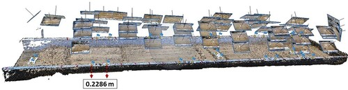
Figure 2 shows the workflow step for generating 3D point clouds using Agisoft Metashape Professional software (1.8.3)(Meloche et al. 2021). Once the photos were taken, they were imported into the software and were aligned to create tie points. Then, gradual selection was applied to filter the point cloud and reduce noise. Three main criteria of the software, named ‘reprojection error’, ‘reconstruction uncertainty’, and ‘projection accuracy’, were adjusted at this stage. The optimal value for each criterion varies according to the project and, for this study, the parameter values used were the following: reprojection error = 0.6 pixel, reconstruction uncertainty = 95.0 pixel, and projection accuracy = 12.0 pixel. The point cloud model was filtered again using the ‘resize’ tool to crop the area of interest and remove unwanted points beyond the area of interest. Once the desired result was achieved, a 3D dense cloud model was created with the ‘Build Dense Cloud’ tool, yielding approximately 13 million points. In contrast to traditional photogrammetry, in which the 3D location of a series of control points should be known, SfM photogrammetry does not require the scale and orientation provided by ground control points (Westoby et al. 2012). The produced 3D point clouds lack the real-world scale because they were generated in a relative image-space dimension. Therefore, to scale the 3D model, the paper targets, with known dimensions, were used as scale bars. Lastly, the camera optimization was applied, and the 3D point cloud model was created with error and accuracy equal to 0.0003 and 0.001 m, respectively. It is important to note that to generate a highly accurate point cloud reconstruction, the targets need to be within as many pictures as possible. Furthermore, good lighting conditions are critical to reduce uncertainty; so, close attention was paid to the photography to avoid shadowing. The 3D model generated from 2D photographs of this study using SfM photogrammetry is shown in Figure 3.

Figure 2. The workflow for 3D point cloud generation using SfM photogrammetry.

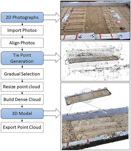
Figure 3. 3D point cloud generation using SfM photogrammetry; targets on each paper are marked using blue flags with a 0.2286 m distance apart.

2.3. Representation of the site surface roughness

Agricultural SSR can be classified into various categories in terms of the magnitude of the soil surface elevation variations and the spatial arrangement of its microelements. These categories can be characterized as random (irregular occurrences of peaks and troughs, Dalla Rosa et al. 2012), isotropic (uniform surface in all directions), and structured surface, which shows systematic difference in elevation due to tillage activities (e.g. row, furrows, or directional pattern, Martinez-Agirre, Álvarez-Mozos, and Giménez 2016). In this study, to easily compare and understand the results of multiple surface roughness profiles, the whole flume was divided into different groups in terms of the level of roughness variations (Figure 4).

Figure 4. The representation of various surface roughness groups by their level of variations.

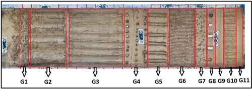
Group 1 (G1) represents a random surface. G2 and G3 show rough and medium-rough row structured surfaces, respectively. G4 and G7 are, respectively, covered by large and small clods on the surface, but in G4, clods have a directional pattern while in G7, clods are randomly oriented. G5 and G10 represent structured surfaces with deep and shallow furrows, respectively. G6 represents a tillage structure, and G9 and G11 are representative of isotropic or very smooth surfaces in the field. Lastly, G8 shows a one-directional rough surface created by large clods.

2.4. Surface roughness data processing

The point clouds obtained by iPhone LiDAR and SfM photogrammetry were pre-processed in the CloudCompare software (version 2.12.0) to extract the scans according to their extent and remove the edge effects. Then, all pre-processed point clouds were analyzed using Roughness from Point Cloud Profiles (RPCP), a specialized software tool, which was developed as a plug-in for surface roughness characterization within the Whitebox Geospatial Analysis Tools (GAT) software version 3.4.0 (Lindsay 2016), to extract the mean RMSH for each surface profile. Only RMSH was chosen for the analysis because this parameter is the most widely used surface roughness parameter in electromagnetic backscattering and microwave radiative transfer models (Li et al. 2020; Zeng et al. 2020; Yang et al. 2021).

The RPCP tool measures surface roughness parameters (RMSH and correlation length) from LiDAR (LAS) files along a series of sampling profiles, which are fitted to a LiDAR point cloud. The user decides on a distance between sampling points and between transects as well as their orientation, and a shapefile polygon can be optionally selected to clip the LAS file to the area of interest. The tool fits a user-defined nth degree polynomial to the point cloud and de-trends the profiles in order to remove the effects of slope or large-scale topography from roughness measurements (Alijani et al. 2021). The de-trended profiles are used to calculate the RMSH by Equation (1). The roughness statistics can be calculated in a multi-azimuth mode, from 0° to 360°. More details about the RPCP tool can be found in Chabot et al. (2018). In the current study, within the RPCP, the distance between profiles and profile sampling were set at 0.025 and 0.01 m, respectively. The RMSH was derived at 90° to match the direction of the pin profiler measurements. (1) $\mathrm{R}\mathrm{M}\mathrm{S}\mathrm{H}=\sqrt{{\displaystyle \frac{1}{n}\sum _{i=1}^n{\left(z_i-\overline{z}\right)}^2}}$(1) where n is the total number of height measurements, z is a single height measurement, and z̄ is the mean of all height measurements (Bryant et al. 2007).

The surface profile photos obtained by pin profiler were processed using a MATLAB graphical user interface, named QuiP (version 8.1.0)(Trudel et al. 2010). This application automatically detects the end of the pin profiler needles and calculates the RMSH and correlation length. However, the detection may not be perfectly aligned to the exact position of the needles, so minor manual correction is required.

The point clouds obtained from SfM photogrammetry generally come with a very large point density (e.g. approximately 17,000 points/m² for this study). Given a very high density of SfM point clouds, the characterization of roughness for individual profiles using SfM point clouds led to a very large RMSH. Therefore, it was not reasonable to calculate each profile’s RMSH separately. Rather than running the RPCP tool for each profile, each roughness group (Figure 4) was used for RMSH extraction in RPCP, so that roughness profiles were clipped to the extent of each group and then were processed for RMSH extraction in RPCP tool. Pin measurements were also averaged for each group (Table 1) to have a one-to-one comparison between groups using the three techniques. The point cloud density exported from iPhone LiDAR would change if the height of iPhone laser scanner changes. Moreover, the 3d Scanner App installed on iPhone has the ability to export data in different resolutions. In this study, a 0.3 m height of LiDAR scanner resulted in the coarse and fine-resolution point clouds with the density of 29 and 209 points/m², respectively. To have a consistent comparison between smartphone-based LiDAR and SfM and pin, the RMSH values obtained from iPhone LiDAR were averaged for each roughness group.

Table 1. Comparison of RMSH obtained by pin profiler and smartphone-based LiDAR for different roughness groups

Roughness group	Profile number	RMSH (cm)
		Pin Profiler	Averaged	SD* (±)	LiDAR (fine resolution)	Averaged	SD (±)	LiDAR (coarse resolution)	Averaged	SD (±)
G1	1	2.11	2.11	–	2.18	2.18	–	3.08	3.08	–
G2	2	3.64	3.36	0.35	3.55	3.44	0.11	2.57	3.04	0.42
	3	3.65			3.52			3.52
	4	3.22			3.32			2.83
	5	2.93			3.36			3.24
G3	6	1.45	1.53	0.12	1.59	2.24	0.92	2.16	2.45	0.67
	7	1.57			2.38			2.74
	8	1.75			2.21			3.23
	9	1.43			3.98			NV*
	10	1.52			1.67			1.46
	11	1.47			1.59			2.64
G4	12	1.34	1.35	0.23	1.09	1.59	0.70	1.16	1.16
	13	1.13			NV			NV
	14	1.58			2.08			NV
G5	15	1.48	1.22	0.37	1.53	1.53		1.5	1.55	0.06
	16	0.95			NV			1.59
G6	17	1.07	1.11	0.13	1.23	1.6	0.53	1.39	2.19	1.16
	18	1.25			2.21			3.52
	19	1			1.37			1.66
G7	20	0.81	0.81	–	1.7	1.7	–	2.18	2.18	–
G8	21	2.31	2.31	–	3.47	3.47	–	2.08	2.08	–
G9	22	0.3	0.3	–	1.15	1.15	–	2.07	2.07	–
G10	23	0.81	0.81	–	2.75	2.75	–	2.81	2.81	–
G11	24	0.69	0.69	–	0.56	0.56	–	0.73	0.73	–

*SD: standard deviation for each profile group. *NV stands for non-value RMSH. The averaged column, in front of each technique, shows the averaged RMSH for each group by that technique.

2.5. Statistical analysis

To analyze the performance of each surface roughness measurement technique, four commonly used statistical indices, including root mean squared error (RMSE), coefficient of determination (R²), correlation coefficient (R), and mean absolute error (MAE), were calculated between each group of roughness measurement techniques. These groups classified as group 1 (pin profiler and SfM photogrammetry), group 2 (pin profiler and fine-resolution LiDAR), group 3 (pin profiler and coarse-resolution LiDAR), group 4 (SfM photogrammetry and fine-resolution LiDAR), and group 5 (SfM photogrammetry and coarse-resolution LiDAR). The error indices were obtained using AgiMetSoft calculator (https://agrimetsoft.com/calculators/).

3. Results

3.1. Comparison of RMSH obtained by pin profiler and smartphone-based LiDAR measurements

The results of the obtained RMSH using pin profiler as well as coarse- and fine-resolution LiDAR are presented in Table 1. As demonstrated, the fine-resolution LiDAR showed the greater value for RMSH for rough surfaces (G2 and G8). This means that rougher surfaces are more sensitive to the density of point clouds. In other words, for rough surfaces, increasing the point density yields higher RMSH. For all other roughness types, lower RMSH were found for fine-resolution point clouds, except for G4 and G5, in which roughness comparison was not possible due to failed experimental procedure which result in a non-value (NV) RMSH for the LiDAR scanner.

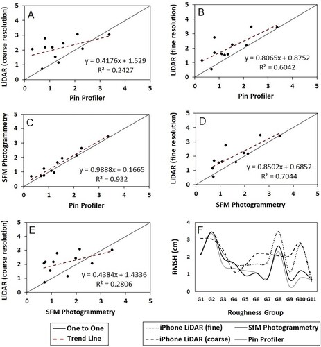
The one-to-one plots of pin and LiDAR measurements show that fine-resolution LiDAR observations are more correlated with pin measurements than coarse-resolution LiDAR scans (Figure 5(a) and (b)). A closer look at Figure 5(f) indicates the strong association between averaged RMSH obtained from LiDAR (fine resolution) and the pin profiler for groups G1, G2, and G11. As previously observed, at G1, roughness elements are randomly oriented and create a rough surface. In contrast, G2 represents a row structured surface similar to what is found in many agricultural fields under row cultivation, where roughness elements follow a consistent peak-and-trough pattern. It should be noted that the orientation of the LiDAR scan line was perpendicular to the row structure, which can result in more reliable roughness estimation (Turner et al. 2014). Therefore, it can be concluded that smartphone-based LiDAR can provide reliable SSR measurements in ploughed agricultural fields when the orientation of the laser scanner is perpendicular to the orientation of cultivation.

Figure 5. (#a)–(e) shows the one-to-one plots of all measured RMSH (cm) obtained by pin, LiDAR (fine & coarse resolutions) and SfM photogrammetry techniques, (f) shows the RMSH variations in each group using pin, SfM and LiDAR (fine & coarse resolutions).

The close match between pin and LiDAR (fine resolution) sensitivity for G1 and G2 can be attributed to the ability of both techniques to capture the roughness variations, as explained by Jester and Klik (2005), who noted that on rough surfaces, the small gaps between aggregates can be followed by pin profiler. The close association between both fine- and coarse-resolution LiDAR with pin profiler can be seen only at G11, where the roughness profile represents an isotropic surface with no variation in elevation height. In general, compared to pin measurements, smartphone-based LiDAR data showed greater values for RMSH. This is likely related to the density of sample points due to the sampling technique, where high density sample points were collected by LiDAR to calculate roughness while only a single 1-m transect was used for pin measurements.

3.2. Comparison of RMSH obtained by pin profiler and SfM photogrammetry

A one-to one plot of RMSH observed by pin and SfM photogrammetry indicates a strong association between these two techniques (Figure 5(c)). Although, the photogrammetry seems to be successfully applied for a range of agricultural fields from smooth to rough surfaces (Gharechelou, Tateishi, and Johnson 2018), this technique showed higher association with pin measurements for some roughness groups. Similar to iPhone LiDAR, SfM has a great match with pin-profile data for G1, G2, and G11. Moreover, the pin-profile and SfM techniques show a close sensitivity for G6 and G7 (Figure 5(f)). This is mainly because G6 and G1, as well as G7 and G2, show in some ways a similar pattern; the first group indicates a random behaviour, and the latter represents a directional field under tillage implementations.

3.3. Comparison of RMSH obtained by smartphone-based LiDAR and SfM photogrammetry

Fine-resolution LiDAR shows a high correlation (R² = 0.70) with SfM data (Figure 5(d)). This association for coarse-resolution point cloud is not significant (R² = 0.28)(Figure 5(e)). This is likely due to the fact that both fine-resolution LiDAR and SfM data have a large point cloud density, leading to a more consistent and parallel comparison compared to coarse-resolution LiDAR. Another important piece of information can be found at Figure 5(f), which indicates a close agreement between fine-resolution LiDAR and SfM for profiles G1, G2, G4, and G11. Unlike G1, G2, and G11, which showed the best association among all measurement techniques, a strong correlation between fine-resolution LiDAR and SfM photogrammetry observed for G4 is unique only to these techniques. This is likely because G4 is an oriented surface, covered by large clods on top of it, that reflects the ability of LiDAR to (1) measure the structure surfaces (Wallace et al. 2016) and (2) to adequately capture the height and texture of above ground features (MacFaden et al. 2012). A closer look at Figure 5(f) indicates that G11 is the only roughness profile that shows a close agreement between coarse-resolution LiDAR and SfM photogrammetry.

3.4. The error statistics of different techniques for surface roughness measurements

Table 2 compares different surface roughness measurement techniques based on four statistical error indices. Since all techniques for surface roughness characterization have a certain amount of measurement error, the quantification of the error was made to investigate whether these techniques were comparable and how close the measurement results were to each other (Bahaaddini et al. 2022). As demonstrated, the pin profiler and SfM photogrammetry showed the highest R and R² and the lowest RMSE and MAE among other groups. According to this table and Figure 5, smartphone-based LiDAR (fine resolution) showed the greatest agreement with SfM photogrammetry but its correlation with the pin profiler is still significant.

Table 2. The statistical error indices for different surface roughness measurement techniques.

Group	Techniques	RMSE	MAE	R	R^2
1	Pin profiler, SfM photogrammetry	0.27	0.22	0.97	0.93
2	Pin profiler, fine-resolution LiDAR	0.83	0.63	0.78	0.60
3	Pin profiler, coarse-resolution LiDAR	1.06	0.84	0.49	0.24
4	SfM photogrammetry, fine-resolution LiDAR	0.67	0.49	0.84	0.70
5	SfM photogrammetry, coarse-resolution LiDAR	0.95	0.82	0.53	0.28

4. Discussion

This study investigated the feasibility of utilizing the novel application of smartphone-based LiDAR and compared it with pin profiler and SfM photogrammetry techniques for SSR characterization. Despite the fact that pin profiler is a common approach for surface roughness characterization, the use of this technique is not suggested for large areas because pin profiler data collection are time consuming, potentially limited in the representation of roughness orientation (Alijani et al. 2021) and requires significant effort to capture long transects, which may limit how representative the approach is for estimating surface roughness spatial variability across large landscapes (Turner et al. 2014). Moreover, limited resolution (cm range) and precision (mm range) are another constraints when contact roughness measurement techniques are used (Poropat 2009; Sturzenegger and Stead 2009; Saricam and Ozturk 2022). Both LiDAR measurements obtained from smartphone-based LiDAR and SfM photogrammetry showed a significant association with pin profiler measurements. However, this association in smartphone-based LiDAR is meaningful only when point cloud data is captured in a fine-resolution mode. Coarse-resolution LiDAR did not show a close agreement with any measurement technique (SfM, pin, fine-resolution smartphone-based LiDAR) for all surface types, except for the isotropic and very smooth surface (G11), for which the RMSH value did not show significant variations with respect to the roughness measurement techniques.

One main aspect of this study revealed that different techniques for measuring surface roughness can produce different sensitivity for surface roughness characterization. The degree of sensitivity in laser scanning approaches depends on several factors such as the type of laser scanners, size of the area under examination, point cloud density, and the orientation of laser scanning. Additionally, camera settings play an important role in the accuracy of 3D photogrammetry models for surface roughness characterization (Kim et al. 2015; Saricam and Ozturk 2022). In this study, camera setting parameters were considered fixed and chosen based on the arbitrary selection of the user because the evaluation of different camera setting parameters on the accuracy of surface roughness characterization obtained from 3D photogrammetry models was outside the scope of this study. However, it is important to consider different camera settings for the same roughness profiles for further surface roughness studies because the optimization and calibration of camera setting parameters may increase the compatibility of SfM photogrammetry with other roughness measurement techniques.

Another aspect of this work demonstrated that the scale of the area under observation can highly impact the results of measuring techniques by which surface roughness data are collected. This study showed that for a small-scale site, composed of multiple surface roughness profiles, characterizing surface roughness for individual small-scale profiles is not effective when roughness data is collected by approaches that generate high density point clouds (like SfM). This is for the reason that high density point clouds will lead to a larger than expected RMSH for individual profiles. So, rather than evaluating separate profiles (small scale), it is recommended to consider similar profiles in a group (large scale) and calculate roughness.

This work also emphasized that different techniques for roughness measurement can show various accuracy for RMSH estimation with respect to surface types. The RMSH obtained from all methods (except for coarse-resolution LiDAR) showed a high correlation for randomly rough (G1) and row-structured rough (G2) surfaces. In addition to these surface types, the RMSH obtained from pin profiler and SfM surveys showed a high correlation for tillage structure (G6) and lumpy small granular (G7) surfaces. Similar results can be seen for oriented lumpy large granular surface (G4) between iPhone LiDAR (fine resolution) and SfM.

In recent years, SfM photogrammetry has emerged as a potentially robust, fast and cost-effective technique for capturing high density point cloud data (Smith, Carrivick, and Quincey 2016; Carrivick and Smith 2019; Schwendel and Milan 2020). This method has been demonstrated to successfully retrieve surface roughness parameters over agricultural fields and showed a comparable accuracy to high precision laser scanning approaches (Martinez-Agirre et al. 2020; An et al. 2021). A higher accuracy in RMSH estimation obtained by SfM photogrammetry for each roughness group is due to the acquisition of a spatially well-distributed and large number of points (Gharechelou, Tateishi, and Johnson 2018). We suggest that the SfM results are reliable for several following reasons: (1) according to our results, SfM was the only method showing the greater correlation with the other two techniques (pin profiles and iPhone LiDAR, Figure 5(c) and (d) and Table 2); (2) the capability of SfM photogrammetry to capture the spatial variability of surface roughness within agricultural fields has been evaluated by several studies (see for example, Snapir, Hobbs, and Waine 2014; Gilliot, Vaudour, and Michelin 2017); (3) a significant association in results between SfM and fine-resolution terrestrial laser scanners shows the SfM application for surface roughness studies (Nouwakpo, Weltz, and McGwire 2016; Fan 2020).

Given a high accuracy of roughness characterization obtained from fine-resolution smartphone-based LiDAR comparable to common and high accuracy methods (pin profiler and SfM photogrammetry) and since this technique is easy to use in the field, especially for rough, wide, and not easily accessible areas, it can be considered as a cost effective and time efficient alternative for rapidly scanning topographical features. The relative ease in the collection and accurate measurement of SSR could be of interest for improving the electromagnetic surface scattering and microwave radiative transfer models that use surface roughness parameters as inputs.

It is necessary to note that, this study was conducted in laboratory conditions, where identical and controlled situations could be maintained over all of the surface profiles. Over real agricultural fields, the characterization of roughness profiles could be more complex, and results may be prone to errors due to instrument specifications and profile length (Adams et al. 2013). Furthermore, the distance between profiles and profile sampling within the RPCP tool should be correctly adjusted according to each surface profile when iPhone LiDAR and SfM techniques are used for point cloud data collection, as these numbers can significantly affect the RMSH value. Considering that not many studies have been conducted for SSR characterization using smartphone-based LiDAR to evaluate and compare the capability of this technique with other common approaches for surface roughness measurements, it is highly beneficial for the microwave remote sensing applications in agriculture to apply this new technology of laser scanning across various fields with different roughness conditions. Therefore, a follow up component for this study aims to evaluate and compare the capability of different SSR measurement techniques over real agricultural fields. Moreover, it is highly suggested to use a high-resolution laser scanner to collect the dense point cloud of roughness profiles to verify the results of the smartphone-based LiDAR over real agricultural fields.

5. Conclusion

In this study, a laboratory experiment consisting of 24 surface roughness profiles constructed in a sand, ranging from smooth to rough, random and structured surfaces were used for surface roughness characterization using three approaches: pin profiler, iPhone LiDAR, and SfM photogrammetry surveys. Our results indicated that large point cloud densities obtained from SfM for individual surface profiles could lead to different values for surface roughness, where the higher the density, the larger the RMSH value. A similar pattern could be observed for point cloud data obtained from iPhone for some profiles (G2 & G8). Moreover, results showed different sensitivity of surface roughness variations with respect to the measurement technique. While the SfM photogrammetry showed the highest association with pin profiler measurements, the correlation between pin profile data and iPhone LiDAR (coarse resolution) data showed the lowest agreement. Furthermore, the results of iPhone LiDAR were more consistent with the SfM technique, particularly for fine-resolution iPhone LiDAR point cloud.

Another important finding of this work highlights the ability of each technique to capture the spatial variability of surface roughness under heterogenous roughness conditions. While all techniques showed a strong agreement in roughness characterization over random and row-structured surfaces, other surface profiles seem to be more sensitive only to specific methods for measuring roughness. However, this study showed that for a very smooth and isotropic surface, changing the roughness measurement technique will not produce a significant difference in the obtained RMSH value. Given the high accuracy of surface roughness estimation obtained from fine-resolution iPhone LiDAR compared to the most commonly used methods for SSR characterization, this technique can be used as a practical alternative tool for roughness parametrization over study fields. These new technologies allow to quantify directly roughness of natural surfaces like soil, snow or ice (Nolan, Larsen, and Sturm 2015) without using effective roughness parameters in surface scattering model. This ultimately benefits remote sensing of geophysical properties by restricting uncertainties in model inversion for remote sensing.

Disclosure statement

No potential conflict of interest was reported by the author(s).

Data availability statement

All roughness data will be available upon request.

Additional information

Funding

Canada First Research Excellence Fund: Food from Thought and the Natural Sciences and Engineering Research Council of Canada (NSERC) fund.

References

- Adams, J. R., A. A. Berg, H. McNairn, and A. Merzouki. 2013. “Sensitivity of C-Band SAR Polarimetric Variables to Unvegetated Agricultural Fields.” Canadian Journal of Remote Sensing 39 (1): 1–16. doi:10.5589/m13-003.
- Alijani, Z., J. Lindsay, M. Chabot, T. Rowlandson, and A. Berg. 2021. “Sensitivity of C-Band SAR Polarimetric Variables to the Directionality of Surface Roughness Parameters.” Remote Sensing 13 (11): 2210. doi:10.3390/rs13112210.
- An, P., K. Fang, Q. Jiang, H. Zhang, and Y. Zhang. 2021. “Measurement of Rock Joint Surfaces by Using Smartphone Structure from Motion (SfM) Photogrammetry.” Sensors 21 (3): 922. doi:10.3390/s21030922.
- Baghdadi, N., N. Holah, and M. Zribi. 2006. “Soil Moisture Estimation Using Multi-Incidence and Multi-Polarization ASAR Data.” International Journal of Remote Sensing 27 (10): 1907–1920. doi:10.1080/01431160500239032.
- Bahaaddini, M., M. Serati, M. H. Khosravi, and B. Hebblewhite. 2022. “Rock Joint Micro-Scale Surface Roughness Characterisation Using Photogrammetry Method.” Journal of Mining and Environment 13 (1): 87–100. doi:10.22044/jme.2022.11669.2155.
- Blaes, X., and P. Defourny. 2008. “Characterizing Bidimensional Roughness of Agricultural Soil Surfaces for SAR Modeling.” IEEE Transactions on Geoscience and Remote Sensing 46 (12): 4050–4061. doi:10.1109/TGRS.2008.2002769.
- Bryant, R., M. S. Moran, D. P. Thoma, C. D. Holifield Collins, S. Skirvin, M. Rahman, K. Slocum, P. Starks, D. Bosch, and M. P. Gonzalez Dugo. 2007. “Measuring Surface Roughness Height to Parameterize Radar Backscatter Models for Retrieval of Surface Soil Moisture.” IEEE Geoscience and Remote Sensing Letters 4 (1): 137–141. doi:10.1109/LGRS.2006.887146.
- Carrivick, J. L., and M. W. Smith. 2019. “Fluvial and Aquatic Applications of Structure from Motion Photogrammetry and Unmanned Aerial Vehicle/Drone Technology.” Wiley Interdisciplinary Reviews: Water 6 (1): e1328. doi:10.1002/wat2.1328.
- Chabot, M., J. Lindsay, T. Rowlandson, and A. A. Berg. 2018. “Comparing the Use of Terrestrial LiDAR Scanners and Pin Profilers for Deriving Agricultural Roughness Statistics.” Canadian Journal of Remote Sensing 44 (2): 153–168. doi:10.1080/07038992.2018.1461559.
- Dai, W., W. Qian, A. Liu, C. Wang, X. Yang, G. Hu, and G. Tang. 2022. “Monitoring and Modeling Sediment Transport in Space in Small Loess Catchments Using UAV-SfM Photogrammetry.” CATENA 214: 106244. doi:10.1016/j.catena.2022.106244.
- Dalla Rosa, J., M. Cooper, F. Darboux, and J. C. Medeiros. 2012. “Soil Roughness Evolution in Different Tillage Systems Under Simulated Rainfall Using a Semivariogram-Based Index.” Soil and Tillage Research 124: 226–232. doi:10.1016/j.still.2012.06.001.
- Das, K., and P. K. Paul. 2015. “Present Status of Soil Moisture Estimation by Microwave Remote Sensing.” Cogent Geoscience 1 (1): 1084669. doi:10.1080/23312041.2015.1084669.
- Davidson, M. W. J., Thuy Le Toan, F. Mattia, G. Satalino, T. Manninen, and M. Borgeaud. 2000. “On the Characterization of Agricultural Soil Roughness for Radar Remote Sensing Studies.” IEEE Transactions on Geoscience and Remote Sensing 38 (2): 630–640. doi:10.1109/36.841993.
- Fan, L. 2020. “A Comparison Between Structure-from-Motion and Terrestrial Laser Scanning for Deriving Surface Roughness: A Case Study on a Sandy Terrain Surface.” The International Archives of Photogrammetry, Remote Sensing and Spatial Information Sciences 42: 1225–1229. doi:10.5194/isprs-archives-XLII-3-W10-1225-2020.
- Fernandez Diaz, J. C., J. Judge, K. C. Slatton, R. Shrestha, W. E. Carter, and D. Bloomquist. 2010. “Characterization of Full Surface Roughness in Agricultural Soils Using Groundbased LiDAR.” IEEE International Geoscience and Remote Sensing Symposium, 4442–4445. doi:10.1109/IGARSS.2010.5652056.
- Gao, Q., and J. Kan. 2022. “Automatic Forest DBH Measurement Based on Structure from Motion Photogrammetry.” Remote Sensing 14 (9): 2064. doi:10.3390/rs14092064.
- García-Gómez, P., S. Royo, N. Rodrigo, and J. R. Casas. 2020. “Geometric Model and Calibration Method for a Solid-State LiDAR.” Sensors 20 (10): 2898. doi:10.3390/s20102898.
- Gharechelou, S., R. Tateishi, and B. A. Johnson. 2018. “A Simple Method for the Parameterization of Surface Roughness from Microwave Remote Sensing.” Remote Sensing 10 (11): 1711. doi:10.3390/rs10111711.
- Gilliot, J.-M., E. Vaudour, and J. Michelin. 2017. “Soil Surface Roughness Measurement: A New Fully Automatic Photogrammetric Approach Applied to Agricultural Bare Fields.” Computers and Electronics in Agriculture 134: 63–78. doi:10.1016/j.compag.2017.01.010.
- Gupta, V. K., and R. A. Jangid. 2011. “Microwave Response of Rough Surfaces with Auto-Correlation Functions, RMS Heights and Correlation Lengths Using Active Remote Sensing.” Indian Journal of Radio & Space Physics 40: 137–146.
- Hajnsek, I., E. Pottier, and S. R. Cloude. 2003. “Inversion of Surface Parameters from Polarimetric SAR.” IEEE Transactions on Geoscience and Remote Sensing 41 (4): 727–744. doi:10.1109/TGRS.2003.810702.
- Hollaus, M., C. Aubrecht, B. Höfle, K. Steinnocher, and W. Wagner. 2011. “Roughness Mapping on Various Vertical Scales Based on Full-Waveform Airborne Laser Scanning Data.” Remote Sensing 3 (3): 503–523. doi:10.3390/rs3030503.
- James, M. R., and S. Robson. 2012. “Straightforward Reconstruction of 3D Surfaces and Topography with a Camera: Accuracy and Geoscience Application.” Journal of Geophysical Research: Earth Surface 117 (F3): 1–17. doi:10.1029/2011JF002289.
- Jester, W., and A. Klik. 2005. “Soil Surface Roughness Measurement—Methods, Applicability, and Surface Representation.” CATENA 64 (2): 174–192. doi:10.1016/j.catena.2005.08.005.
- Kellner, J. R., J. Armston, M. Birrer, K. C. Cushman, L. Duncanson, C. Eck, C. Falleger, et al. 2019. “New Opportunities for Forest Remote Sensing Through Ultra-High-Density Drone Lidar.” Surveys in Geophysics 40 (4): 959–977. doi:10.1007/s10712-019-09529-9.
- Kim, D. H., G. V. Poropat, I. Gratchev, and A. Balasubramaniam. 2015. “Improvement of Photogrammetric JRC Data Distributions Based on Parabolic Error Models.” International Journal of Rock Mechanics and Mining Sciences 80: 19–30. doi:10.1016/j.ijrmms.2015.09.007.
- Kim, S.-B., L. Tsang, J. T. Johnson, S. Huang, J. J. van Zyl, and E. G. Njoku. 2012. “Soil Moisture Retrieval Using Time-Series Radar Observations Over Bare Surfaces.” IEEE Transactions on Geoscience and Remote Sensing 50 (5): 1853–1863. doi:10.1109/TGRS.2011.2169454.
- King, J., C. Derksen, P. Toose, A. Langlois, C. Larsen, J. Lemmetyinen, P. Marsh, B. Montpetit, A. Roy, and N. Rutter. 2018. “The Influence of Snow Microstructure on Dual-Frequency Radar Measurements in a Tundra Environment.” Remote Sensing of Environment 215: 242–254. doi:10.1016/j.rse.2018.05.028.
- King, F., R. Kelly, and C. G. Fletcher. 2022. “Evaluation of LiDAR-Derived Snow Depth Estimates from the IPhone 12 Pro.” IEEE Geoscience and Remote Sensing Letters 19: 1–5. doi:10.1109/LGRS.2022.3166665.
- Kong, D., C. Saroglou, F. Wu, P. Sha, and B. Li. 2021. “Development and Application of UAV-SfM Photogrammetry for Quantitative Characterization of Rock Mass Discontinuities.” International Journal of Rock Mechanics and Mining Sciences 141: 104729. doi:10.1016/j.ijrmms.2021.104729.
- Landy, J. C., D. Isleifson, A. S. Komarov, and D. G. Barber. 2015. “Parameterization of Centimeter-Scale Sea Ice Surface Roughness Using Terrestrial LiDAR.” IEEE Transactions on Geoscience and Remote Sensing 53 (3): 1271–1286. doi:10.1109/TGRS.2014.2336833.
- Lavoie, A., F. Bonn, R. Fournier, J. Deslandes, I. Beaudin, and A. Michaud. 2006. “Spaceborne Observation and Modeling of Erosion and Non-Point Source Pollution in Agricultural Catchments Draining Into Lakes.” Global Developments in Environmental Earth Observation from Space Proceedings 25: 287–298.
- Le Morvan, A., M. Zribi, N. Baghdadi, and A. Chanzy. 2008. “Soil Moisture Profile Effect on Radar Signal Measurement.” Sensors 8 (1): 256–270. doi:10.3390/s8010256.
- Li, N., C.P. Ho, J. Xue, L.W. Lim, G. Chen, Y.H. Fu, and L.Y.T. Lee. 2022. “A Progress Review on Solid-State LiDAR and Nanophotonics-Based LiDAR Sensors.” Laser & Photonics Reviews 16(11): 2270057. doi:10.1002/lpor.202270057.
- Li, Y., S. Yan, N. Chen, and J. Gong. 2020. “Performance Evaluation of a Neural Network Model and Two Empirical Models for Estimating Soil Moisture Based on Sentinel-1 SAR Data.” Progress In Electromagnetics Research C 105: 85–99. doi:10.2528/PIERC20071601.
- Lindsay, J. B. 2016. “Whitebox GAT: A Case Study in Geomorphometric Analysis.” Computers & Geosciences 95: 75–84. doi:10.1016/j.cageo.2016.07.003.
- Luetzenburg, G., A. Kroon, and A. A. Bjørk. 2021. “Evaluation of the Apple IPhone 12 Pro LiDAR for an Application in Geosciences.” Scientific Reports 11 (1): 1–9. doi:10.1038/s41598-021-01763-9.
- Luhmann, T., C. Fraser, and H.-G. Maas. 2016. “Sensor Modelling and Camera Calibration for Close-Range Photogrammetry.” ISPRS Journal of Photogrammetry and Remote Sensing 115: 37–46. doi:10.1016/j.isprsjprs.2015.10.006.
- MacFaden, S. W., J. P. M. O’Neil-Dunne, A. R. Royar, J. W. T. Lu, and A. G. Rundle. 2012. “High-Resolution Tree Canopy Mapping for New York City Using LIDAR and Object-Based Image Analysis.” Journal of Applied Remote Sensing 6 (1): 063567. doi:10.1117/1.JRS.6.063567.
- Martinez-Agirre, A., J. Álvarez-Mozos, and R. Giménez. 2016. “Evaluation of Surface Roughness Parameters in Agricultural Soils with Different Tillage Conditions Using a Laser Profile Meter.” Soil and Tillage Research 161: 19–30. doi:10.1016/j.still.2016.02.013.
- Martinez-Agirre, A., J. Álvarez-Mozos, M. Milenković, N. Pfeifer, R. Giménez, J. Manuel Valle, and Á Rodríguez. 2020. “Evaluation of Terrestrial Laser Scanner and Structure from Motion Photogrammetry Techniques for Quantifying Soil Surface Roughness Parameters Over Agricultural Soils.” Earth Surface Processes and Landforms 45 (3): 605–621. doi:10.1002/esp.4758.
- McNairn, H., A. Merzouki, A. Pacheco, and J. Fitzmaurice. 2012. “Monitoring Soil Moisture to Support Risk Reduction for the Agriculture Sector Using RADARSAT-2.” IEEE Journal of Selected Topics in Applied Earth Observations and Remote Sensing 5 (3): 824–834. doi:10.1109/JSTARS.2012.2192416.
- Meloche, J., A. Royer, Al. Langlois, N. Rutter, and V. Sasseville. 2021. “Improvement of Microwave Emissivity Parameterization of Frozen Arctic Soils Using Roughness Measurements Derived from Photogrammetry.” International Journal of Digital Earth 14 (10): 1380–1396. doi:10.1080/17538947.2020.1836049.
- Merzouki, A., H. McNairn, and A. Pacheco. 2011. “Mapping Soil Moisture Using RADARSAT-2 Data and Local Autocorrelation Statistics.” IEEE Journal of Selected Topics in Applied Earth Observations and Remote Sensing 4 (1): 128–137. doi:10.1109/JSTARS.2011.2116769.
- Mikalai, Z., D. Andrey, H. S. Hawas, Н Tеtiana, and S. Oleksandr. 2022. “Human Body Measurement with the IPhone 12 Pro LiDAR Scanner.” AIP Conference Proceedings 2430 (1): 090009–090016. doi:10.1063/5.0078310.
- Moreno, R. G., M. C. Díaz Álvarez, A. T. Alonso, S. Barrington, and A. S. Requejo. 2008. “Tillage and Soil Type Effects on Soil Surface Roughness at Semiarid Climatic Conditions.” Soil and Tillage Research 98 (1): 35–44. doi:10.1016/j.still.2007.10.006.
- Murtiyoso, A., P. Grussenmeyer, T. Landes, and H. Macher. 2021. “First Assessments Into the Use of Commercial-Grade Solid State Lidar for Low Cost Heritage Documentation.” The International Archives of the Photogrammetry, Remote Sensing and Spatial Information Sciences XLIII-B2-2021, 43: 599–604. doi:10.5194/isprs-archives-XLIII-B2-2021-599-2021.
- Nolan, M., C. Larsen, and M. Sturm. 2015. “Mapping Snow Depth from Manned Aircraft on Landscape Scales at Centimeter Resolution Using Structure-from-Motion Photogrammetry.” The Cryosphere 9 (4): 1445–1463. doi:10.5194/tc-9-1445-2015.
- Nouwakpo, S. K., M. A. Weltz, and K. McGwire. 2016. “Assessing the Performance of Structure-from-Motion Photogrammetry and Terrestrial LiDAR for Reconstructing Soil Surface Microtopography of Naturally Vegetated Plots.” Earth Surface Processes and Landforms 41 (3): 308–322. doi:10.1002/esp.3787.
- Oh, Y. 2004. “Quantitative Retrieval of Soil Moisture Content and Surface Roughness from Multipolarized Radar Observations of Bare Soil Surfaces.” IEEE Transactions on Geoscience and Remote Sensing 42 (3): 596–601. doi:10.1109/TGRS.2003.821065.
- Poropat, G. V. 2009. “Measurement of Surface Roughness of Rock Discontinuities.” In Proceedings of the 3rd CANUS Rock Mechanics Symposium, Toronto, edited by G. Grasselli, and M. S. Diederichs, 3976. 3rd Canada-US rock mechanics symposium, Toronto, Canada.
- Roberts, K. C., J. B. Lindsay, and A. A. Berg. 2019. “An Analysis of Ground-Point Classifiers for Terrestrial Lidar.” Remote Sensing 11 (16): 1915. doi:10.3390/rs11161915.
- Rodríguez-Caballero, E., Y. Cantón, S. Chamizo, A. Afana, and A. Solé-Benet. 2012. “Effects of Biological Soil Crusts on Surface Roughness and Implications for Runoff and Erosion.” Geomorphology 145: 81–89. doi:10.1016/j.geomorph.2011.12.042.
- Rychkov, I., J. Brasington, and D. Vericat. 2012. “Computational and Methodological Aspects of Terrestrial Surface Analysis Based on Point Clouds.” Computers & Geosciences 42: 64–70. doi:10.1016/j.cageo.2012.02.011.
- Sakai, T., E. Birhane, B. Abebe, and D. Gebremeskel. 2021. “Applicability of Structure-from-Motion Photogrammetry on Forest Measurement in the Northern Ethiopian Highlands.” Sustainability 13 (9): 5282. doi:10.3390/su13095282.
- Saricam, I. T., and H. Ozturk. 2022. “Joint Roughness Profiling Using Photogrammetry.” Applied Geomatics, 14(4):1–15. doi:10.1007/s12518-022-00454-y.
- Schwendel, A. C., and D. J. Milan. 2020. “Terrestrial Structure-from-Motion: Spatial Error Analysis of Roughness and Morphology.” Geomorphology 350: 106883. doi:10.1016/j.geomorph.2019.106883.
- Seidel, D., and C. Ammer. 2014. “Efficient Measurements of Basal Area in Short Rotation Forests Based on Terrestrial Laser Scanning Under Special Consideration of Shadowing.” IForest - Biogeosciences and Forestry 7 (4): 227–232. doi:10.3832/ifor1084-007.
- Smith, M. W., J. L. Carrivick, and D. J. Quincey. 2016. “Structure from Motion Photogrammetry in Physical Geography.” Progress in Physical Geography 40 (2): 247–275. doi:10.1177/0309133315615805.
- Snapir, B., S. Hobbs, and T. W. Waine. 2014. “Roughness Measurements Over an Agricultural Soil Surface with Structure from Motion.” ISPRS Journal of Photogrammetry and Remote Sensing 96: 210–223. doi:10.1016/j.isprsjprs.2014.07.010.
- Sturzenegger, M., and D. Stead. 2009. “Close-Range Terrestrial Digital Photogrammetry and Terrestrial Laser Scanning for Discontinuity Characterization on Rock Cuts.” Engineering Geology 106 (3–4): 163–182. doi:10.1016/j.enggeo.2009.03.004.
- Tao, H., Q. Chen, Z. Li, J. Zeng, and X. Chen. 2017. “Improvement of Soil Surface Roughness Measurement Accuracy by Close-Range Photogrammetry.” Transactions of the Chinese Society of Agricultural Engineering 33 (15): 162–167.
- Tatsumi, S., K. Yamaguchi, and N. Furuya. 2021. “ForestScanner: A Mobile Application for Measuring and Mapping Trees with LiDAR-Equipped IPhone and IPad.” Methods in Ecology and Evolution, 00: 1–7. doi:10.1111/2041-210X.13900.
- Tavani, S., A. Billi, A. Corradetti, M. Mercuri, A. Bosman, M. Cuffaro, T. Seers, and E. Carminati. 2022. “Smartphone Assisted Fieldwork: Towards the Digital Transition of Geoscience Fieldwork Using LiDAR-Equipped IPhones.” Earth-Science Reviews 227: 103969. doi:10.1016/j.earscirev.2022.103969.
- Teppati Losè, L., A. Spreafico, F. Chiabrando, and F. G. Tonolo. 2022. “Apple LiDAR Sensor for 3D Surveying: Tests and Results in the Cultural Heritage Domain.” Remote Sensing 14 (17): 4157. doi:10.3390/rs14174157.
- Tontini, A., L. Gasparini, and M. Perenzoni. 2020. “Numerical Model of Spad-Based Direct Time-of-Flight Flash Lidar CMOS Image Sensors.” Sensors 20 (18): 5203. doi:10.3390/s20185203.
- Trudel, M., F. Charbonneau, F. Avendano, and R. Leconte. 2010. “Quick Profiler (QuiP): A Friendly Tool to Extract Roughness Statistical Parameters Using a Needle Profiler.” Canadian Journal of Remote Sensing 36 (4): 391–396. doi:10.5589/m10-070.
- Turner, R., R. Panciera, M. A. Tanase, K. Lowell, J. M. Hacker, and J. P. Walker. 2014. “Estimation of Soil Surface Roughness of Agricultural Soils Using Airborne LiDAR.” Remote Sensing of Environment 140: 107–117. doi:10.1016/j.rse.2013.08.030.
- Vinci, A., F. Todisco, L. Vergni, and D. Torri. 2020. “A Comparative Evaluation of Random Roughness Indices by Rainfall Simulator and Photogrammetry.” Catena 188: 104468. doi:10.1016/j.catena.2020.104468.
- Wallace, L., A. Lucieer, Z. Malenovský, D. Turner, and P. Vopěnka. 2016. “Assessment of Forest Structure Using Two UAV Techniques: A Comparison of Airborne Laser Scanning and Structure from Motion (SfM) Point Clouds.” Forests 7 (3): 62. doi:10.3390/f7030062.
- Wang, X., H. Lyu, T. Mao, W. He, and Q. Chen. 2022. “Point Cloud Segmentation from IPhone-Based LiDAR Sensors Using the Tensor Feature.” Applied Sciences 12 (4): 1817. doi:10.3390/app12041817.
- Westoby, M. J., J. Brasington, N. F. Glasser, M. J. Hambrey, and J. M. Reynolds. 2012. “Structure-from-Motion’ Photogrammetry: A Low-Cost, Effective Tool for Geoscience Applications.” Geomorphology 179: 300–314. doi:10.1016/j.geomorph.2012.08.021.
- Yang, M., H. Wang, C. Tong, L. Zhu, X. Deng, J. Deng, and K. Wang. 2021. “Soil Moisture Retrievals Using Multi-Temporal Sentinel-1 Data Over Nagqu Region of Tibetan Plateau.” Remote Sensing 13 (10): 1913. doi:10.3390/rs13101913.
- Zeng, J., K.-S. Chen, C. Cui, and X. Bai. 2020. “A Physically Based Soil Moisture Index from Passive Microwave Brightness Temperatures for Soil Moisture Variation Monitoring.” IEEE Transactions on Geoscience and Remote Sensing 58 (4): 2782–2795. doi:10.1109/TGRS.2019.2955542.
- Zheng, X., L. Li, S. Chen, T. Jiang, X. Li, and K. Zhao. 2019. “Temporal Evolution Characteristics and Prediction Methods of Spatial Correlation Function Shape of Rough Soil Surfaces.” Soil and Tillage Research 195: 104417. doi:10.1016/j.still.2019.104417.
- Zimmerman, T., and J. K. Miller. 2021. “UAS-SfM Approach to Evaluate the Performance of Notched Groins Within a Groin Field and Their Impact on the Morphological Evolution of a Beach Nourishment.” Coastal Engineering 170: 103997. doi:10.1016/j.coastaleng.2021.103997.