Assessing Landsat-8 atmospheric correction schemes in low to moderate turbidity waters from a global perspective

ABSTRACT

Atmospheric correction is one of the major challenges in ocean color remote sensing, thus threatening comprehensive evaluation of water quality within aquatic environments. In this study, five state-of-the-art atmospheric correction (AC) processors (i.e. Acolite, C2RCC, iCOR, L2gen, and Polymer) were applied to Operational Land Imager (OLI) Landsat-8 scenes and evaluated against in situ measurements across various types of waters worldwide. A total of 262 matchups between in situ measured and satellite-derived remote sensing reflectance (R_rs) at 20 sites were obtained between August 2013 and August 2021. Classification of optical water types (OWTs) was carried out using in situ measurements with matched satellite observations. OWT-specific analysis demonstrated that L2gen produced the most accurate R_rs with R² ≥ 0.74 and root mean squared error (RMSE) ≤ 0.0018 sr^–1 for the four visible bands of OLI, followed by Polymer, C2RCC, iCOR, and Acolite. In terms of R_rs spectral similarity, C2RCC yielded the lowest spectral angle (SA) of 8.55°, followed by L2gen (SA = 9.20°). The advantage and disadvantage of each AC scheme were discussed. Recommendations to improve the accuracy for atmospheric correction were made, such as polarization observations and concurrent aerosol and ocean color measurements.

KEYWORDS:

• Atmospheric correction
• Landsat-8
• ocean color
• remote sensing reflectance

1. Introduction

Although coastal waters occupy only 7% of the total ocean surface, they serve as essential hubs for human and wildlife activities and are critical components of global ecosystems (Osterholz et al. 2021). Given their importance in human habitation, resource provisioning, cultural practice, and carbon sequestration, they play a significant role in achieving the Sustainable Development Goals (SDGs). However, global trends point to continued deterioration of coastal waters caused by pollution and eutrophication (Chen et al. 2017). Therefore, it is very important to conduct systematic, large-scale, and continuous researches on them from a long-term perspective (Jamet et al. 2011). With the advantage of synoptic views of marine biosphere over large spatial and temporal scales, ocean color remote sensing represents a unique tool to provide vital insights into the linkage between human activity and coastal marine environments. Its products can serve for comprehensive evaluation of water quality and greatly facilitate assessment of coastal ecosystems (Marrari, Hu, and Daly 2006; Volpe et al. 2007; Malenovsky et al. 2012; Platt 2008; Mouw et al. 2015).

It is well-known that top-of-atmosphere signals received by ocean color satellite sensors contained approximately 90% atmospheric and 10% oceanic information (Gordon et al. 1985). Therefore, atmospheric correction (AC) is one of the key procedures in the application of quantitative ocean color remote sensing. The black pixel assumption algorithm performs well and can reach the goal of 5% uncertainty for remote sensing reflectance (R_rs, unit sr^–1) in the blue and green wavelengths for open oceanic waters (Gordon and Wang 1994; Mélin 2019). However, AC over coastal waters is challenged by the presence of continental aerosols, bottom reflection, and adjacency of land (Renosh et al. 2020; Siegel et al. 2000; Shanmugam 2012). Numerous efforts have been made to minimize those perturbing effects (Xue et al. 2021). For example, wavelengths in the ultraviolet (He et al. 2012) or in the short-wave infrared (SWIR) (Wang 2007; Wang and Shi 2007) were introduced to improve the determination of the aerosol model in highly turbid waters. Fixed reflectance models and spatial homogeneity of aerosol were also proposed for moderately turbid waters (Hu, Carder, and Muller-Karger 2000; Ruddick, Ovidio, and Rijkeboer 2000). With the availability of powerful computation facilities, numerical and statistical optimization algorithms were developed (Chomko and Gordon 1998; Guanter et al. 2010; Son and Wang 2012; Wang et al. 2020). To ensure the continuity and consistency with past and present ocean color missions, it is essential to validate and assess the existent AC schemes across various types of waters with different hydrodynamic and atmospheric conditions.

Performance of AC schemes has been validated over turbid waters for different satellite sensors, such as Medium Resolution Imaging Spectrometer (MERIS) (Jaelani et al. 2015), Sea-Viewing Wide Field-of-View Sensor (SeaWiFS) (Jamet et al. 2011), Moderate Resolution Imaging Spectroradiometer-Aqua (MODIS-Aqua) (Zhang et al. 2018; Goyens, Jamet, and Schroeder 2013), Geostationary Ocean Color Imager (GOCI) (Mu et al. 2019; Huang et al. 2019), OLI (Wei et al. 2018; Xu et al. 2020), Sentinel-2 MultiSpectral Instrument (MSI) (Konig, Hieronymi, and Oppelt 2019; Warren et al. 2019; Martins et al. 2017; Pflug et al. 2019; Pereira-Sandoval et al. 2019), and Ocean and Land Color Instrument (OLCI) (Renosh et al. 2020; Mograne et al. 2019). Various levels of uncertainties were found from those validation practice over optically diverse waters. Previous studies focused on assessing waters in North America and Europe (Ilori, Pahlevan, and Knudby 2019; Xu et al. 2020; Warren et al. 2019; Pereira-Sandoval et al. 2019; Mograne et al. 2019). However, the optimal AC scheme over turbid waters from a global perspective needs further investigation, such as in China Seas and off South America.

In this study, we aim to compare five state-of-the-art AC processors for OLI commonly used in the field of ocean color, i.e. Acolite, C2RCC, iCOR, L2gen, and Polymer. Extensive datasets over global oceans are involved, including Europe, Africa, North America, South America, Asia, and Oceania. The most suitable AC method for each region based on precision or spectral similarity needs will be proposed. To achieve the goal, in situ measurements across global waters from different sources are utilized, including Aerosol Robotic Network-Ocean Color (AERONET-OC), SeaWiFS bio-optical archive and storage system (SeaBASS), Marine Optical BuoY (MOBY), National Satellite Ocean Application Service of China (NSOAS), and our research cruises. Optical classification for different water bodies is implemented using R_rs spectra.

2. Data and method

2.1. In situ observation

In situ observations from a total of 20 sites around the world, as shown in Figure 1, were collected between August 2013 and August 2021, coinciding with OLI/Landsat 8 overpasses. Table 1 lists the information for those 20 stations. Figure 2 shows OLI-derived true color composites for those stations across various types of waters with different hydrodynamic conditions. AERONET-OC provides normalized water-leaving radiance (nL_w) at globally distributed offshore sites. Quality-assured nL_w (Level 2.0) data from 12 AERONET-OC sites were used. Equation (1)(1) $R_{rs}\left(\lambda \right)={\displaystyle \frac{L_w\left(\lambda \right)}{E_s\left(\lambda \right)}={\displaystyle \frac{n{L}_w\left(\lambda \right)}{F_0\left(\lambda \right)}}}$(1) was used to convert nL_w to R_rs. SeaBASS is a well moderated and documented archive for bio-optical data, which is operated by National Aeronautics and Space Administration (NASA). SeaBASS data were downloaded from https://seabass.gsfc.nasa.gov/. MOBY, anchored off Lanai, Hawaii, has provided vicarious calibration data in near real time for ocean color sensors since 1996. MOBY-measured L_w data were acquired from the National Oceanic and Atmospheric Administration (NOAA). NSOAS deployed an ocean color instrument, named Cruise for Apparent Optical Properties (CruiseAOP), to collect R_rs at a fixed station off Muping, China, which became operational since January 2020 and is about 25 kilometers away from the coastline with a water depth of about 12 m. Two field campaigns were conducted in May-June and August 2021 in the South China Sea (SCS), respectively, during which CruiseAOP was also used for R_rs measurements.

Figure 1. Map of 20 sites (solid circles) with matched in situ radiometric measurements within ± 2 h of Landsat-8 overpasses. Dots of the same color represent sites given the same name listed in Table 1. Names of six locations whose remote sensing reflectance (R_rs) spectra are shown in Figure 7 are annotated. Please refer to Table 1 for details. (For interpretation of the references to color in this figure legend, the reader is referred to the web version of this article.)

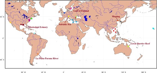
Figure 2. OLI/Landsat-8 derived RGB composites for the 20 stations listed in Table 1.

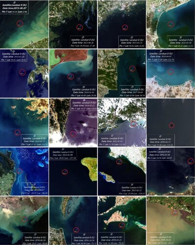
Table 1. Information for locations with matched in situ radiometric and Landsat 8 OLI measurements, including station number, station name and their abbreviations, latitude, and longitude.

Station #	Station name	Abbreviation	Latitude	Longitude
①	Southern North Sea of Europe-Strait of Dover	SoD	51.53°	2.96°
②	West Baltic Sea-Norrkoping Sea	NS	58.59°	17.47°
③	East Baltic Sea-Gulf of Finland	GoF	59.95°	24.93°
④	Northern Mediterranean-Adriatic Sea	AS	45.31°	12.51°
⑤	Central Mediterranean-Ionian Sea	IS	34.37°∼38.81°	20.42°∼29.39°
⑥	West Black Sea-Eastern Lacul Razim	ELR	44.60°	29.36°
⑦	West Black Sea-Varna Estuary	VE	43.04°	28.19°
⑧	Northwest Yellow Sea-Muping	MP	37.68°	121.70°
⑨	Northern Yellow Sea	NYS	37.42°	124.74°
⑩	Western Sea of Japan-South Korea's waters	SK	35.47°	129.62°
⑪	Northern South China Sea-Yangjiang Waters	YJ	21.69°∼21.70°	112.30°∼112.44°
⑫	Central South China Sea	CSCS	13.06°∼20.19°	113.53°∼117.95°
⑬	Great Barrier Reef	GBR	–18.52°	146.39°
⑭	Hawaiian Islands	HI	20.81°∼20.82°	–157.20°∼–157.19°
⑮	Northeast Pacific-Channel Islands of California	CIoC	33.56°	–118.12°
⑯	West Atlantic-Southern Caribbean	SC	10.50°	–64.67°
⑰	Northwest Atlantic-Mississippi Estuary	ME	28.87°	–90.48°
⑱	Northwest Atlantic-Chesapeake Bay	CB	33.41°∼36.9°	–78.51°∼–75.71°
⑲	Northwest Atlantic-Marthas Vineyard	MV	41.30°	–70.55°
⑳	West Atlantic-La Plata-Parana River	LPPR	–34.76°	–56.54°

The CruiseAOP instrument was equipped with three pre-calibrated radiometers (TriOS RAMSES-ARC-VIS), one for irradiance and the other two for radiance. The instrument has a rotatable component which can automatically control the observation geometry of the sensors. The total above-surface radiance (L_t), downwelling sky radiance (L_s), and downwelling incident irradiance (E_s) in the spectral range of 325–944 nm were simultaneously measured at an interval of 15 minutes. For each time stamp, 15 spectral scans were recorded for L_t, L_s, and E_s, respectively. The averaged spectra were then obtained. All measurements followed the NASA ocean optics protocols to minimize sun glint perturbations (Mueller et al. 2003). According to Lee et al. (2016), R_rs was calculated from (1) $R_{rs}\left(\lambda \right)={\displaystyle \frac{L_w\left(\lambda \right)}{E_s\left(\lambda \right)}={\displaystyle \frac{n{L}_w\left(\lambda \right)}{F_0\left(\lambda \right)}}}$(1) (2) $R_{rs}\left(\lambda \right)={\displaystyle \frac{L_w\left(\lambda \right)}{E_s\left(\lambda \right)}={\displaystyle \frac{L_t-{\rho }_s{L}_s\left(\lambda \right)}{E_s\left(\lambda \right)}-\mathrm{\Delta }}}$(2) where ρ_s is the Fresnel reflectance at the air–sea interface and was determined following Mobley (1999). F₀ represents the solar irradiance of perpendicular incident outside the atmosphere at mean sun-Earth distance. Δ is related to a second-order correction and determined by setting the spectrally averaged R_rs between 900 and 920 nm to 0 here.

2.2. Satellite data processing

On 11 February 2013, the Landsat-8 satellite was launched as a joint initiative between the U.S. Geological Survey (USGS) and NASA, carrying the Operational Land Imager (OLI) and the Thermal Infrared Sensor (TIRS). OLI measures top of atmosphere (TOA) radiance in 9 wavebands in the visible to shortwave infrared (SWIR) domain at a spatial resolution of 30 m. Landsat-8 OLI collection 1 level 1 data were downloaded from USGS. Five AC algorithms, namely Acolite, C2RCC, iCOR, L2gen, and Polymer, were implemented. Acolite, C2RCC and L2gen directly output R_rs while iCOR and Polymer yielded dimensionless water-leaving reflectance (ρ_w) that was transformed into R_rs via R_rs= ρ_w/π. R_rs at 443, 482, 561, and 655 nm was generated.

2.3. Optical water types

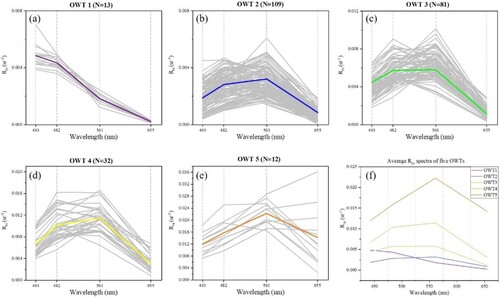
To meet the need for an assessment of AC processors across widely variable coastal water conditions, the fuzzy C-means (FCM) clustering algorithm proposed by Vantrepotte et al. (2012) was employed for the classification of optical water types (OWTs). As shown in Figure 3, five OWTs were achieved for all data involved in this study based on their spectral shape and m. They were numbered sequentially from blue, oligotrophic waters to moderately eutrophic, sediment-rich waters with an overall trend of increasing chlorophyll and optical complexity.

Figure 3. Averaged R_rs spectra for the five optical water types (OWTs).

To enable direct inter-comparison among the AC processors for each OWT, the following steps were carried out. First of all, pairs of matched in situ and satellite-derived R_rs were defined. If R_rs retrieval from any AC algorithm fails, the data pair would be rejected. 13 pairs of data were retained for OWT 1, 109 for OWT 2, 81 for OWT 3, 32 for OWT 4, and 12 for OWT 5. Secondly, the five algorithms were ranked based on statistical measures. Finally, the comprehensive ranking of each AC algorithm for each band was obtained.

2.4. Match-up analysis

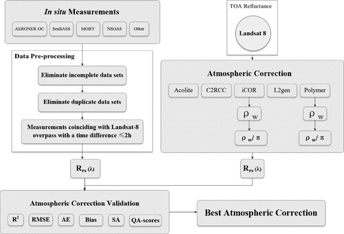
The flowchart of match-up analysis between in situ measurements and satellite observations is shown in Figure 4. For some in situ measurements, R_rs at certain bands was not available and thus discarded. Duplicated data were removed since different data sources were involved. The spatial and temporal windows were set to 5 × 5 and ±2 h, respectively. The matching exercise followed the approach proposed by Bailey and Werdell (2006). For each matched pair, the median of R_rs (λ) over a 5 × 5 pixel window centered at the station was used. A median is better than a mean because the former is less sensitive to spikes. Several flags were checked for satellite-derived R_rs, including cloud shadow, stray light, and sun glint. Finally, 262 pairs of matched field measurements and OLI observations were obtained, with 184 from AERONET-OC, 21 from SeaBASS, 33 from MOBY, 11 from Muping, and 13 from the SCS.

Figure 4. Flowchart for matchup analysis and satellite data processing in this study.

2.5. Statistical analysis

Along with slope, intercept, and determination coefficient (R²), the following statistical measures, i.e. bias, absolute error (AE), and root mean square error (RMSE), were used for the performance assessment of the five AC algorithms: (3) $\mathrm{b}\mathrm{i}\mathrm{a}\mathrm{s}\left(\text{\%}\right)={\displaystyle \frac{1}{n}\ast {\sum }_{i=1}^n{\displaystyle \frac{\left(R_{rs}{{}^{sat}}_i\left(\lambda \right)-R_{rs}{{}^{meas}}_i\left(\lambda \right)\right)}{R_{rs}{{}^{meas}}_i\left(\lambda \right)}}\ast 100}$(3) (4) $\mathrm{A}\mathrm{E}={\displaystyle \frac{1}{n}\ast {\sum }_{i=1}^n\left|R_{rs}{{}^{sat}}_i\left(\lambda \right)-R_{rs}{{}^{meas}}_i\left(\lambda \right)\right|}$(4) (5) $\mathrm{R}\mathrm{M}\mathrm{S}\mathrm{E}=\sqrt{{\displaystyle \frac{{\sum }_{i=1}^n{\left(R_{rs}{{}^{sat}}_i\left(\lambda \right)-R_{rs}{{}^{meas}}_i\left(\lambda \right)\right)}^2}{n}}}$(5) where n is the number of match-ups, R_rs^sat denotes satellite-derived R_rs using a specific AC algorithm, and R_rs^meas denotes field measured R_rs. Spectral Angle (SA) (Keshava 2004) was introduced to quantify the similarity between satellite-derived and in situ measured R_rs spectra. SA is insensitive to amplitude and calculated from (6) $\mathrm{S}\mathrm{A}={\cos }^{-1}{\displaystyle \frac{\sum _{i=1}^n{R}_{rs}{{}^{meas}}_i\times R_{rs}{{}^{sat}}_i}{\sqrt{\sum _{i=1}^n{\left(R_{rs}{{}^{meas}}_i\right)}^2}\sqrt{\sum _{i=1}^n{\left(R{{}_{rs}^{sat}}_i\right)}^2}}}$(6) where i denotes the ith band of OLI. Smaller SA indicates higher similarity. If R_rs for an OLI wavelength is not available, data for the nearest wavelength were used instead.

3. Description for AC algorithms

TOA radiance received by ocean color satellite sensors (L_toa) can be decomposed into several terms as follows: (7) $L_{toa}\left(\lambda \right)=L_R\left(\lambda \right)+L_A\left(\lambda \right)+L_{ra}\left(\lambda \right)+T\left(\lambda \right)L_g\left(\lambda \right)+L_b\left(\lambda \right)+t_d\left(\lambda \right)L_{wc}\left(\lambda \right)+t_d\left(\lambda \right)L_w\left(\lambda \right)$(7) L_R(λ) is the Rayleigh scattering of atmospheric molecules. L_A(λ) is the aerosol scattering in the atmosphere. L_ra(λ) is the multiple scattering of aerosol-molecular interaction. L_g(λ) is the reflection of sun glint on the sea surface entering the sensor field of view, also known as specular reflectance. L_b is the reflection from bottom. L_wc(λ) is the reflection of white bubble cloud entering the sensor field of view, also known as white cap reflection. L_w(λ) is water-leaving radiance. T(λ) is the direct transmittance, also known as beam transmittance. t_d(λ) is the atmospheric attenuation coefficient between sea surface and sensor, also known as atmospheric diffuse transmittance.

Acolite (version 20210114) is a generic image-base processor developed by the Royal Belgian Institute of Natural Sciences (RBINS). It does not need external inputs, such as aerosol optical thickness (AOT). The default dark spectrum fitting (DSF) approach was utilized (Vanhellemont 2019). This scheme assumes a homogeneous atmosphere. An automated method is performed to predict atmospheric path reflectance based on multiple dark pixels selected in a scene (such as ground surface shadows or water pixels). This approach requires the presence of SWIR bands to work over scenes with only turbid waters (Vanhellemont and Ruddick 2018).

The Case 2 Regional Coast Color (C2RCC) processor involves a multi-sensor per-pixel artificial neural network to perform the inversion of L_w from L_toa, as well as the retrieval of inherent optical properties (IOPs) (Doerffer and Schiller 2007; Brockmann et al. 2016). Characterization of optically complex waters through its IOPs as well as of coastal atmospheres is performed to parameterize radiative transfer models for water and atmosphere. A large dataset for reflectance at water surface is produced, which is then used as lower boundary conditions for the radiative transfer calculation in the atmosphere. A database of 5 million cases is generated, which forms the basis for neural network training. It can be imbedded into the SeNtinel Application Platform (SNAP, V6.0) software. The default settings were used for all images.

Image correction for atmospheric effects (iCOR) offers the ability of AC over inland, coastal, and transitional waters (Guanter, Gonzalez-Sanpedro, and Moreno 2007). It first identifies land and water pixels using a band threshold approach. Scene-specific aerosol optical thickness (AOT) is obtained following the SCAPE-M algorithm (Guanter, Gonzalez-Sanpedro, and Moreno 2007). An adjacency correction can optionally be applied using the SIMilarity Environmental Correction (SIMEC) approach (Sterckx et al. 2015). A MODerate resolution atmospheric TRANsmission (MODTRAN 5) look-up table is built (Berk et al. 2006), which requires ancillary information as inputs, such as solar and viewing angles and digital elevation model. If the above steps fail, Rayleigh scattering correction is automatically initiated with a default AOT of 0.1. Proper terrestrial pixel distributions are needed to obtain the best results. iCOR can be implemented as a plugin in the SNAP software (V6.0). In this study, the default settings were applied and the adjacency correction was implemented.

Level 2 generator (L2gen) is a combination of NASA atmospheric correction algorithms. It employs bio-optical models and resolves AC in an iterative process (Gordon and Wang 1994; Bailey, Franz, and Werdell 2010). An iterative scheme is exploited to estimate the aerosol radiance at the near-infrared (NIR) and/or shortwave infrared (SWIR) bands to relax the limitation of the ‘dark pixel’ assumption. In this study, OLI bands centered at 865 and 2201 nm were exploited. This NIR-SWIR band combination has been proven to yield the most robust R_rs in moderately turbid waters (Pahlevan et al. 2017). L2gen is a built-in program for SeaWiFS Data Analysis System (SeaDAS, V7.5).

The Polynomial based algorithm applied to MERIS (Polymer) is specially designed for oceanic waters with and without the presence of sun glint (Steinmetz, Deschamps, and Ramon 2011). Compared with other AC algorithms, it can thus improve valid data availability. It employs a spectra-matching optimization method on a pixel-by-pixel basis. It relies on two models, one for spectral reflectance of atmosphere and sun glint and the other for water reflectance in the visible wavebands. The bio-optical water reflectance model is extended to NIR wavebands using the similarity spectrum for turbid waters (Ruddick et al. 2006). The parameters for the two models are tuned iteratively to produce the best fit. Default settings for Polymer (V4.14) were used.

4. Results

4.1. Validation of R_rs from the five AC schemes

Figure 5 shows the scatter plots of in situ measured against OLI-derived R_rs in the visible region from the five AC schemes. The statistical results are summarized in Table 2. The histograms for AE, bias, RMSE, and R² are displayed in Figure 6. It can be seen that the performance of the five AC algorithms indicates discrepancies for different wavelengths. For the 443 nm band, L2gen demonstrates the best performance with the largest R² of 0.74, a slope closest to 1, and the smallest RMSE, AE and bias, followed by Polymer, C2RCC, iCOR, and Acolite. For the 482 nm band, Polymer produces the best result with the largest R² of 0.84 and the smallest RMSE. For the green band centered at 561 nm, L2gen also yields the best match between in situ and satellite-derived R_rs with a R² of 0.97, a RMSE of 0.0013 sr^–1, and a bias of –7%. In terms of R² and bias, C2RCC illustrates better performance than Polymer. The worst performance is found from iCOR. The performance of Acolite is ranked the fourth among the five algorithms. With respect to the red band centered at 655 nm, R_rs data from L2gen show the best agreement with in situ measurements with a slope closest to 1 and the smallest bias. Polymer and C2RCC have similar performance. Relatively large deviation from the 1:1 relationship is observed for R_rs from Acolite and iCOR while the latter agrees better with field measurements than the former. For all AC matchups, the scatter points are relatively dispersed for R_rs at 443 nm, which is consistent with previous findings (Pahlevan et al. 2021).

Figure 5. Scatter plots of satellite-derived versus in situ measured R_rs for visible bands of OLI/Landsat-8. The orange dashed lines refer to the 1:1 relationship and other colored lines represent the best-fitted relationships. Note that the scale for each band is different.

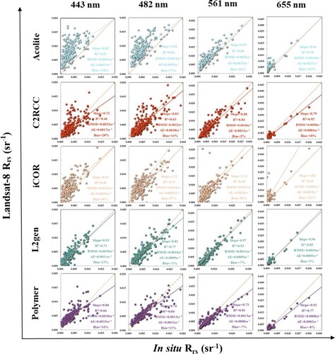
Figure 6. Histograms for absolute error (AE), bias, root mean square error (RMSE), and R² for satellite-derived vs in situ measured R_rs at visible bands of OLI/Landsat-8.

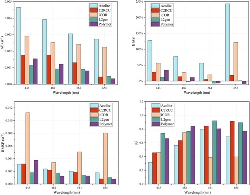
Table 2. Statistical results for remote sensing reflectance (R_rs) at four visible bands of Operational Lands Imager (OLI) Landsat 8 using five atmospheric correction (AC) algorithms, including Acolite, C2RCC, iCOR, L2gen, and Polymer. Statistical measures for comparison between in situ and satellite measurements include slope, intercept, R², root mean square error (RMSE), absolute error (AE), bias, spectral angle (SA), quality assurance (QA) score. N denotes the number of data samples. Best metrics for each band are highlighted in bold.

AC	Band	Slope	Intercept	R^2	RMSE (sr^–1)	AE (sr^–1)	Bias	SA (°)	QAS	N
Acolite	443	0.82	0.0055	0.31	0.0031	0.0047	128%	13.7	0.65	227
	482	0.82	0.0047	0.56	0.0024	0.0039	77%
	561	0.93	0.0031	0.80	0.0020	0.0031	56%
	655	0.96	0.0028	0.70	0.0018	0.0027	243%
C2RCC	443	0.72	0.0024	0.46	0.0032	0.0017	28%	8.6	0.98	262
	482	0.83	0.0010	0.63	0.0022	0.0018	14%
	561	0.88	0.0004	0.84	0.0018	0.0013	5%
	655	0.79	0.0004	0.92	0.0008	0.0004	18%
iCOR	443	0.83	0.0035	0.46	0.0112	0.0029	56%	19.4	0.60	253
	482	1.32	–0.0003	0.75	0.0034	0.0025	27%
	561	1.11	0.0007	0.39	0.0051	0.0024	20%
	655	1.62	0.0017	0.40	0.0081	0.0022	122%
L2gen	443	0.93	0.0010	0.74	0.0018	0.0011	13%	9.2	0.81	233
	482	0.82	0.0007	0.77	0.0018	0.0009	–3%
	561	0.97	–0.0003	0.92	0.0013	0.0009	–7%
	655	0.96	0.0002	0.89	0.0010	0.0005	1%
Polymer	443	0.80	0.0023	0.66	0.0038	0.0015	34%	10.8	0.96	261
	482	0.74	0.0019	0.84	0.0013	0.0012	11%
	561	0.73	0.0012	0.81	0.0013	0.0008	–7%
	655	0.92	0.0001	0.77	0.0008	0.0003	–8%

In general, R_rs for all bands is overestimated by Acolite and iCOR. AE and bias for R_rs from Acolite and iCOR are much larger than from other three algorithms. Note that L2gen exhibits near-zero biases at 482, 561, and 655 nm, which corroborates the findings of previous studies (Pahlevan et al. 2021). As shown in Table 3, L2gen has the best performance at 443 and 482 nm with the smallest AE while Polymer has the best performance at 561 and 655 nm. Polymer-derived versus in situ R_rs points are evenly scattered around the 1:1 line with R²s > 0.7 for all bands. L2gen produces the lowest bias, AE and RMSE for four bands while tends to overestimate R_rs at 443 and 482 nm, which is consistent with recent studies (Ilori, Pahlevan, and Knudby 2019; Xu et al. 2020). To further evaluate algorithm performance, radar charts displaying statistical measures for each band are shown in Figure 7. Each vertex of the hexagon represents a statistical parameter. The length of a spoke is proportional to the magnitude of a statistical measure. Results further away from the center represent higher metric values, demonstrating better performance than those closer to it. In this scenario, all statistical parameters can be superimposed to objectively assess the performance of each AC algorithm from a global perspective. It can be seen that the area for L2gen is the largest for all bands, indicative of the best comprehensive performance. The performance ranking is followed by Polymer, C2RCC, iCOR, and Acolite in order. Therefore, it can be concluded that L2gen has the best performance among the five AC schemes.

Figure 7. Radar map for each visible band of OLI in terms of bias, slope, intercept, R², RMSE, and AE.

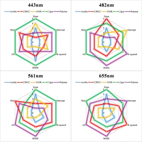
Table 3. ACs with the best performance for each station in terms of SA and average of AE (AAE) between in situ and satellite measured R_rs. The number in brackets in the second column indicates the number of matched in situ and OLI measured R_rs. The sixth to ninth columns represent ACs with the best performance for each visible band of Landsat 8 OLI for each station.

Station	Region with match-ups	Best AC	SA (°)	AAE (sr^–1)	443 nm	482 nm	561 nm	655 nm
①	SoD (5)	L2gen	5.20	0.0005	L2gen	L2gen	L2gen	L2gen
②	NS (14)	C2RCC	9.10	0.0004	C2RCC	C2RCC	Polymer	C2RCC
③	GoF (20)	L2gen	11.71	0.0005	L2gen	L2gen	Polymer	C2RCC
④	AS (40)	Polymer	7.06	0.0009	L2gen	L2gen	Polymer	Polymer
⑤	LS (4)	C2RCC	3.20	0.0006	C2RCC	Polymer	C2RCC	C2RCC
⑥	ELR (35)	C2RCC	6.72	0.0012	C2RCC	L2gen	L2gen	Polymer
⑦	VE (21)	C2RCC	7.19	0.0007	L2gen	L2gen	Polymer	Polymer
⑧	MP (11)	C2RCC	8.75	0.002	C2RCC	Polymer	Polymer	Polymer
⑨	CYS (2)	C2RCC	6.75	0.0004	C2RCC	C2RCC	L2gen	C2RCC
⑩	SK (1)	iCOR	1.00	0.0164	Polymer	Polymer	C2RCC	C2RCC
⑪	YJ (4)	Polymer	6.01	0.0053	L2gen	L2gen	L2gen	L2gen
⑫	CSCS (9)	Polymer	12.00	0.0082	Polymer	Polymer	Polymer	Polymer
⑬	GBR (6)	Polymer	5.26	0.0024	Polymer	Polymer	Polymer	Polymer
⑭	HI (8)	C2RCC	3.26	0.0009	L2gen	L2gen	Polymer	Polymer
⑮	CIoC (16)	Polymer	4.26	0.0010	L2gen	L2gen	Polymer	Polymer
⑯	SC (4)	C2RCC	8.44	0.0005	C2RCC	C2RCC	Polymer	C2RCC
⑰	ME (19)	C2RCC	5.11	0.0007	C2RCC	C2RCC	L2gen	C2RCC
⑱	CB (8)	L2gen	8.63	0.0003	L2gen	L2gen	L2gen	Polymer
⑲	MV (29)	C2RCC	6.81	0.0013	C2RCC	Polymer	Polymer	Polymer
⑳	LPPR (7)	iCOR	2.37	0.0046	Acolite	C2RCC	C2RCC	C2RCC

4.2. Relative performance assessments for five optical water types

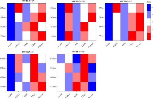
Figure 8 shows relative performance assessments of AC algorithms for the five OWTs. Overall, L2gen demonstrates good performance for all five OWTs, especially at 443 and 482 nm. In contrast, among the five algorithms, Acolite generally produces the poorest results for all five OWTs except for OWT5. It appears that Acolite is suitable for sediment-rich waters, consistent with previous findings (Renosh et al. 2020; Pereira-Sandoval et al. 2019). Polymer performs well for OWTs 1 to 3, especially at 561 nm, where it always illustrates the best results. Note that the performance of Polymer compromises in turbid coastal waters, such OWTs 4 and 5. C2RCC-derived R_rs shows the highest accuracy for OWT 2 among the five algorithms and indicates the best performance at 655 nm. This can be attributed to the precise handling of low R_rs values in the red bands by the neural network of C2RCC. The performance of iCOR has low ranking for OWTs 1 to 4. However, iCOR shows good performance for R_rs at 443 and 482 nm for OWT 5, ranking the first and second, respectively.

Figure 8. Performance assessment of five AC algorithms for five optical water types (OWTs). Different colors indicate their rankings for the visible bands of OLI/Landsat 8. Warm color indicates better performance. (For interpretation of the references to color in this figure legend, the reader is referred to the web version of this article.)

Figure 9 shows the comparison between averaged R_rs spectra from in-situ and satellite observations using different AC algorithms for the five OWTs. L2gen-generated R_rs spectra agree well with in situ measurements. In general, Acolite-obtained R_rs spectra deviate the most from in situ data for all OWTs except for OWT 5. This further verifies that Acolite is suitable for the treatment of highly turbid water bodies. The spectral shape of Polymer-derived R_rs is in good agreement with in situ measurements of OWTs 1 to 3, especially at 561 and 655 nm. Nevertheless, its performance degrades for OWTs 4 to 5. R_rs from iCOR is generally overestimated. Table 4 lists the most suitable OWT-specific AC algorithm for each wavelength based on spectral shape preference via calculating SA. It can be seen that the spectral similarity for R_rs from Polymer is the highest for OWT 1 with an SA of 1.15°. C2RCC has the smallest SAs for OWTs 2 and 4 with SAs of 4.92° and 1.31°, respectively. L2gen-derived R_rs has the most similar spectral shapes to the in-situ data for OWTs 3 and 5 with SAs of 3.94° and 1.57°, respectively. These findings are consistent with those shown in Figure 9.

Figure 9. Comparison between averaged R_rs spectra from in-situ and satellite observations using different AC algorithms for five OWTs.

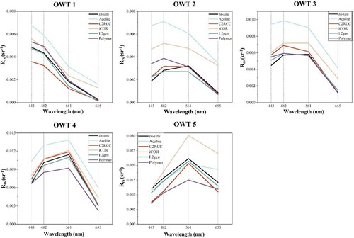
Table 4. AC algorithm assessment for different optical water types (OWTs) using SA and the optimal algorithm is highlighted in bold. The best band-specific algorithm for each OWT is also presented. The number in brackets in the first column indicates the number of matched in situ and OLI-measured R_rs for each OWT.

OWTs (of match-ups)	ACs	SA (°)	443 nm	482 nm	561 nm	655 nm
OWT 1 (13)	Acolite	8.26	Polymer	L2gen	Polymer	C2RCC
	C2RCC	1.42
	iCOR	7.95
	L2gen	3.29
	Polymer	1.15
OWT 2 (109)	Acolite	14.87	C2RCC	L2gen	Polymer	C2RCC
	C2RCC	4.92
	iCOR	15.14
	L2gen	7.71
	Polymer	13.91
OWT 3 (81)	Acolite	9.77	L2gen	Polymer	Polymer	C2RCC
	C2RCC	4.60
	iCOR	7.00
	L2gen	3.94
	Polymer	5.34
OWT 4 (32)	Acolite	7.16	Polymer	L2gen	L2gen	L2gen
	C2RCC	1.31
	iCOR	4.18
	L2gen	2.12
	Polymer	4.63
OWT 5 (12)	Acolite	8.48	iCOR	L2gen	L2gen	L2gen
	C2RCC	8.03
	iCOR	9.33
	L2gen	1.57
	Polymer	6.03

4.3. Comparison of R_rs spectra for different stations

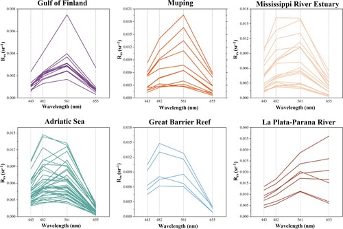
In situ measured R_rs spectra with matched satellite measurements for six sites from five continents, three in the northern hemisphere and three in the southern hemisphere, respectively, across various types of waters are shown in Figure 10. R_rs from the Gulf of Finland (GoF) was generally lower than 0.008 sr^–1 and peaked in the green region with a minimum in the blue region < 0.0015 sr^–1. These spectral features were attributed to high contents of colored dissolved organic matter (CDOM), whose absorption at 412 nm varied between 0.8 and 1.6 m^–1 (Kowalczuk 1999). R_rs spectra from Muping and Mississippi River Estuary were similar and characterized by peaks at 561 nm that varied in the range of 0.003–0.02 sr^–1 and 0.0026–0.016 sr^–1 for the two stations, respectively. Note that there were several cases when R_rs peaked at 482 nm and was < 0.003 sr^–1 for both stations, which was caused by the landward movement of clear blue waters around them. For the Adriatic Sea and Great Barrier Reef stations, the peak wavelength of R_rs spectra varied between 482 and 561 nm. The peak values also demonstrated relatively large ranges, almost an order of magnitude. R_rs spectra from Muping, Mississippi River Estuary, Adriatic Sea, and Great Barrier Reef were typical for coastal waters influenced by both freshwater discharge and local ocean circulation (Mélin et al. 2016). R_rs spectra from the La Plata-Parana River were characterized by high values in the red domain. R_rs spectral peak at 561 gradually disappeared and the entire spectra were uplifted, which was associated with high loads of suspended sediment and agreed well with the findings in the Yangtze River Estuary (Pan, Shen, and Wei 2018).

Figure 10. In situ measured R_rs spectra at six sampling sites. Only those with matched satellite observations are shown here.

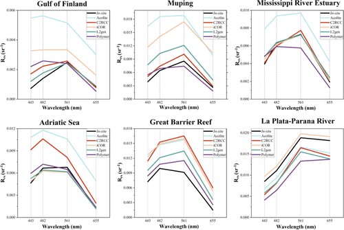
SAs computed for all stations over global oceans are illustrated in Figure 11. L2gen and C2RCC achieve the lowest median SA of 8° while the former has a smaller interquartile range and thus tighter distribution than the latter. Averaged in situ R_rs spectra and the matched satellite observations for the six stations are shown in Figure 12. The best-performing AC algorithm for all stations in terms of SA and average of AE (AAE) is summarized in Table 3. Apparently, great discrepancies can be recognized for different AC schemes. For example, C2RCC demonstrates the best performance for the Muping station with an SA of 8.75° and an AAE of 0.002 sr^–1. For the Great Barrier Reef station, R_rs spectra from Polymer have the highest similarity to in situ data. Among the five algorithms, R_rs spectra from Acolite generally deviate the most from in situ measurements. On the other hand, it deserves noting that the performance of AC algorithms varies for different bands. Table 3 lists the optimal AC algorithm for each band at each station. Except for several cases where L2gen or Polymer produces the best R_rs retrievals for all bands, mixed AC solutions are observed. Note that Acolite yields the best R_rs at 443 nm in the very turbid La Plata-Prana River. It may therefore be advantageous to seek a fit-for-purpose AC that estimates satisfactory R_rs retrievals in only one or two individual bands for specific applications.

Figure 11. Spectral angle for each AC processor. Smaller spectral angle would imply more similar shape. The red line represents the median and the boxes cover the 25–75% range. The upper and lower whiskers represent values outside the middle 50% (excluding outliers), defined as 1.5 × interquartile range (1.5 IQR). Box plot in depicts median (horizontal line), interquartile range (box), 1.5 × interquartile range (error bars), and outliers (black dots) which fall more than 1.5 times the interquartile range. (For interpretation of the references to color in this figure legend, the reader is referred to the web version of this article.)

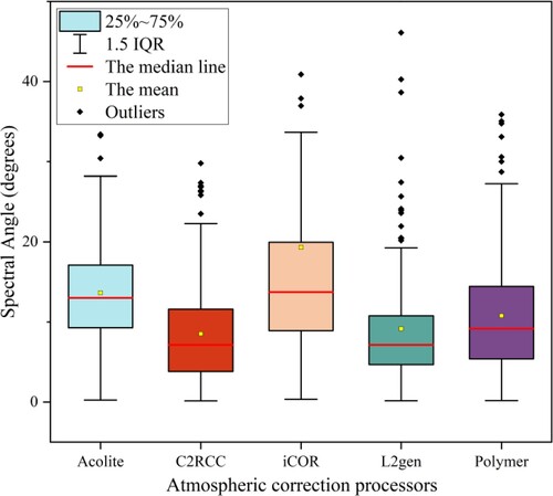
Figure 12. Comparison between averaged R_rs spectra from field measurements and satellite observations using different atmospheric correction algorithms.

4.4. Inter-comparison of satellite-derived R_rs spectra

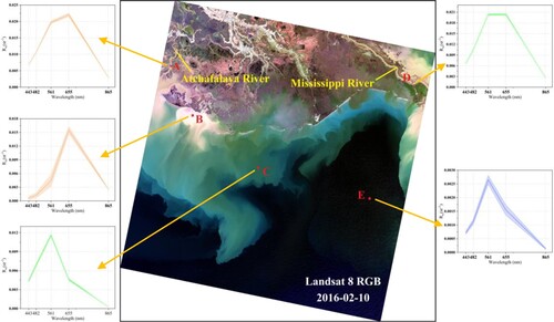
The quality assurance (QA) evaluation system developed by Wei, Lee, and Shang (2016) is introduced here to further assess the quality of R_rs from each AC algorithm in terms of spatial distribution for different OWTs. It was applied to a satellite scene on 20 February 2016 with clear sky conditions covering the region that receives freshwater and nutrients via two large rivers, namely the Mississippi River (MR) and the Atchafalaya River (AR), as illustrated in Figure 13. A previous study showed that riverine nitrogen input accounted for 80% of the total nitrogen load on this shelf (Xue et al. 2013), making the MR-AR system a major source of nutrients to support local primary production (Joshi and D’Sa 2020). The unique absorption, scattering, and fluorescence properties of optically active constituents affect light fields, resulting in variations of R_rs spectra. The yellowish-brown color (areas A and D in Figure 13) represents mineral-rich water with a R_rs peak at 655 nm. R_rs for area B has a higher rate of change than for area A in the visible domain. In this dynamic mixing zone where CDOM and sediment-rich plume water mixed with oligotrophic offshore waters, apparent discrepancies in water color can be observed. The green color over area C in Figure 13 represents waters with more contents of phytoplankton than other areas with R_rs peaks in the green region (e.g. 561 nm). For area E, R_rs peaks at 561 nm while an order of magnitude smaller than those for area C.

Figure 13. True color composite for 10 February 2016 over the area affected by the Atchafalaya River and the Mississippi River. Landsat-8 OLI-derived R_rs spectra for five locations, i.e. A–E, representing different water conditions are shown. The colored line denotes the averaged R_rs for the 30 × 30 pixels and the shaded color denotes standard deviation. (For interpretation of the references to color in this figure legend, the reader is referred to the web version of this article.)

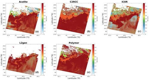
Figure 14 shows the comparison of QA scores for R_rs derived from different AC processors. It can be seen that R_rs retrieved from all algorithms has higher accuracy in offshore waters than in nearshore waters, which is likely associated with high loads of suspended sediment in nearshore water. Note that R_rs over areas with high sediment was masked in the L2gen algorithm although L2gen-produced R_rs generally demonstrates high quality. In the vicinity of our sampling site (around area C), QA score is high. C2RCC-derived R_rs demonstrates the best spatial smoothness than those from other algorithms. In clear blue waters, C2RCC and Polymer has good performance, followed by Acolite. In contrast, QA scores for R_rs from L2gen and iCOR are even lower than 0.3 in some areas. These findings are related to the mechanism of AC algorithms mentioned above.

Figure 14. Quality assurance score (QAS) for OLI/Landsat 8-measured R_rs from different atmospheric correction processors. The scene was collected on 10 February 2016. The higher QAS, the better data quality.

5. Discussion

5.1. Uncertainties of matchup analysis

Although field data are usually considered as ‘ground truth’, they also contain some uncertainties, like incomplete calibration, non-standard instrument operation, ship shadow, white cap, sun glint, and the Fresnel reflection of sky radiance (Mobley 1999). A recent study reported that radiometric measurements at water surface may have an uncertainty of 5–50% in the visible region (Alikas et al. 2020). Another study showed that even the same measurement technique was used with well-calibrated instruments, the results differed by up to 10% from AERONET-OC (Tilstone et al. 2020). This phenomenon can be explained by the following reasons. Firstly, some uncontrollable factors, such as sea wave and underwater mixing process, caused rapid changes in the aquatic light field and introduced uncertainties (Ackleson 2003). Secondly, variations in water depth and optical properties of the water column may result in inaccurate measurements (Mishra et al. 2007). Thirdly, in situ data from different sources were used in this study. They were determined with hyperspectral radiometers from different manufacturers with different calibration histories and data processing procedures also differed. All these factors would introduce potential errors to field data. The spatial difference between field and satellite observations is well-known since the latter covers much larger areas than the former. Furthermore, the diversity of benthic substrates is a potential source of differences between them since variations in optical properties for different benthic habitats can be anticipated (Karpouzli and Malthus 2003; Kutser, Dekker, and Skirving 2003). In optically shallow waters, different types of benthic habitats (like seagrass, bare sand, and coral) can affect the accuracy of in situ measurements (Zeng et al. 2022). For example, sites in the Great Barrier Reef in Figure 10 show greater variations in blue wavelengths than in other wavelengths, which may be due to uncertainty in the measurement of surface radiation (i.e. changes in sky conditions) or strong absorption of benthic corals in blue wavelengths.

Temporal dynamics are one of the key characteristics that ocean and atmosphere differ from land (Cui et al. 2014). The time difference between in situ and satellite measurements has also persisted. Although in situ data collected within ±2 h of satellite overpass were used to represent the matching results, ocean color satellite data are often biased in turbid coastal waters of complex physical and bio-optical properties. For example, rapid changes in sediment re-suspension caused by wind, tide, river plume, or precipitation during the 2 h period can affect the optical properties of water column. Moreover, the extent to which wind and tidal changes affect sediment re-suspension depends on the local bottom topography and varies for different coastal regions (Choi et al. 2012; Shi and Wang 2009; Nezlin and DiGiacomo 2005). An alternative is to use matching records with the same collection time. However, the 16-day revisit frequency of Landsat 8 poses limitations.

Hence, increasing the amount of available data may provide a feasible solution, which can decrease the potential uncertainties of in situ measurements during inappropriate conditions. Time series collection of in situ data can be made through a large number of regular and continuous field work. This requires various shared ocean color field observations (such as SeaBASS and MOBY) to harmonize data inputs from various sources, expand data reserves, unify data formats, and simplify the process of data submission and acquisition. These efforts would greatly facilitate future atmospheric correction assessments. Using a combination of various methods to create a large data pool may minimize systematic errors in the performance evaluation (Pahlevan et al. 2021). Therefore, it is possible to characterize the optical properties and their spatiotemporal variations over oceans, which, in turn, can improve the accuracy of AC.

5.2. Advantages and disadvantages for each AC processor

5.2.1. Acolite

The most recent version of Acolite updated the look-up table (LUT) for dark spectral fitting, using the default continental and maritime aerosol models, and also supports the addition of additional aerosol models (Vanhellemont 2019). Acolite has been validated over Pléiades images in turbid coastal waters in Zeebrugge and the results showed that R_rs products from the newly developed DSF algorithm were superior to those from the SWIR method. But this algorithm can hardly obtain valid values in clear water (Vanhellemont and Ruddick 2018). DSF is similar to ‘black NIR’ or ‘black SWIR’ (Gordon and Wang 1994). Involving land pixels in the processing window provides better performance than using any type of water pixels. Therefore, there is a reasonable explanation for its poor performance for OWTs 1 to 4 while good for OWT 5 since OWT 5 is closer to land. In addition, the inaccurate aerosol calculation is a potential cause of errors. A key step of DSF is to find all ‘dark’ pixels in the entire scene. Vanhellemont and Ruddick (2018) emphasized that using samples with dark pixels would greatly facilitate AC. However, Acolite dynamically identifies the darkest pixels for each band and does not implement adjacency correction. Therefore, land pixels may contaminate R_rs of adjacent water pixels.

5.2.2. C2RCC

C2RCC generally produced good performance in various regions and bands, ranked the third behind L2gen and Polymer. Unlike Acolite and L2gen, C2RCC had almost no pixel windows rejected since the dependence of the algorithm on input parameters is relatively low. However, C2RCC tended to highly underestimate R_rs for OWTs 1 and 5. This could be related to the fact that the optical conditions of the training set (Soriano-González et al. 2022) were closer to those of OWTs 2 to 4. However, the optical conditions of OWTs 1 and 5 included in this study may differ from those in the training dataset for C2RCC, which limited the use of this processor in eutrophic and oligotrophic waters (Ligi et al. 2017).

However, the present version of the C2RCC processor does not correct for the effect of sun glint. Through feedbacks from the scientific community to characterize the scope and limitation, C2RCC is constantly improved and the future version is expected to improve the accuracy of the blue band and correct for sun glint effect. Since the good performance of C2RCC is related to its capability of capturing slight effects during calibration, new machine-learning solutions should be considered (Pahlevan et al. 2021). Feasible measures include improving forward radiative transfer modeling and exploring the latest architectures (e.g. optimization functions, loss functions, activation functions) or models (e.g. Convolutional Neural Network, Recurrent Neural Network).

5.2.3. iCOR

iCOR is an image-based algorithm. It does not require profound knowledge of radiative transfer and absolute calibration of sensors, which makes it easy to implement. However, this image-based process requires the radiance from cloud shadow over water and land pixels to derive relevant parameters for the correction, which are not always present. As shown in Figure 9, iCOR generally overestimated reflectance for five OWTs due to limited land pixels for aerosol estimation. The extrapolation of land pixels probably underestimated atmospheric path radiation in coastal waters. It is very likely that these corrections returned default values of aerosol optical thickness (Warren et al. 2019). This may help to explain the poor performance of iCOR at offshore stations, such as Gulf of Finland and Muping. Note that adjacency effect influenced by land cover type and its seasonal variation, topography and other environmental conditions can affect the estimation of aerosol types and thickness, especially in inland and coastal waters, and further influence the accuracy of AC (Pahlevan et al. 2021). At present, iCOR is the only processor that corrects adjacency effect.

5.2.4. L2gen

As illustrated in Figure 5 and Table 2, L2gen achieved the best agreement with field measurements and was the most stable and balanced among the five algorithms for all OWTs. This can be explained by the following reasons: (1) Aerosol data used in L2gen were mainly obtained from AERONET-OC (Ahmad et al. 2010) that is also the major source of in situ data for matchup in this study; (2) The built-in bio-optical model and iterative scheme with NIR and SWIR switching options contribute to the stability of retrieval; (3) The effective standard flagging system can remove low-quality pixels and improve the retrieval quality. However, L2gen also showed systematic underestimation for all OWTs except for OWT 3, as shown in Figures 6 and 12. This phenomenon could be related to adjacency effects or uncertainties in estimating the aerosol contribution because of low signal-to-noise ratio propagation into the blue band when extrapolated from NIR and SWIR bands. They both led to overestimation of aerosols and retrieval of negative or low R_rs (Ibrahim et al. 2018). Therefore, uncertainties still exist in L2gen-retrieved R_rs data. L2gen requires an accurate understanding of aerosol types to obtain high-quality R_rs retrievals. Hence, uncertainties for L2gen-derived R_rs are mainly determined by uncertainties in aerosol LUTs, spectral extrapolations, and absorbing aerosols (Gordon, Du, and Zhang 1997; Franz et al. 2015).

In view of the abovementioned potential sources of uncertainties, Pahlevan et al. (2014) and Franz et al. (2015) investigated vicarious calibration gains for OLI, which apparently improved the accuracy of R_rs. However, alternative calibration gains also introduced some uncertainties as a result of algorithm failure caused by residual effects from cloud shadow or overcorrection for aerosol contribution in one or more visible band. Overcorrection usually occurs when water-leaving radiance is not negligible for bands used to estimate aerosol contributions (Amin et al. 2009). Pahlevan et al. (2014) found that alternative calibration gains could also result in overcorrection of L2gen-derived R_rs at 443 nm.

5.2.5. Polymer

The Polymer algorithm assumes that the Angstrom coefficient of aerosol scattering is 1.0 (Zhang et al. 2018). From the perspective of global statistics, Angstrom coefficient usually varies between 0.5 and 1.3 (Hu, Lee, and Franz 2012). For clear open oceanic waters, it is close to 1.0. Nevertheless, it will deviate from 1.0 for coastal waters and estuaries, resulting in incorrect spectral shape of aerosol reflectance and then leading to errors in the retrieved R_rs. As reported by Steinmetz, Deschamps, and Ramon (2011), inappropriate estimation of wind speed at each pixel would yield negative reflectivity. Furthermore, Polymer simplifies that reflectance can be modeled as a function of two parameters, i.e. chlorophyll-a concentration and a coefficient (g) to account for backscattering variability (Zhang et al. 2018). In clear open oceanic waters where optical properties are mainly determined by chlorophyll-a, like OWTs 1 to 3, the algorithm demonstrated good performance, especially at 561 and 655 nm. Obvious overestimation can be clearly seen for R_rs at 443 and 482 nm. This is related to the following reasons: (1) Insufficient correction for strong Rayleigh scattering in the blue to green spectral domain; (2) The spectral optimization did not account for contributions of CDOM to IOPs, other than chlorophyll-a (Steinmetz and Ramon 2018). In turbid coastal waters, like OWTs 4 to 5, changes in optical properties are affected not only by phytoplankton and their appendage, but also by other substances, such as suspended inorganic particles and CDOM (Babin et al. 2003; Siegel and Michaels 1996; Jiang et al. 2014). The assumptions made in Polymer are not applicable. Polymer would thus greatly underestimate R_rs as different IOP models produced different phytoplankton concentration outputs (Windle et al. 2022).

5.3. Potential improvements towards AC processors

As discussed above, each AC scheme has their own advantage and disadvantage. The choice of optimal AC for specific region varies, especially for coastal turbid waters. Relative large errors may be expected when data outside the range of those used for algorithm development are involved. Therefore, optical classification of OWTs is essential to improve the accuracy of different AC algorithms. In addition, there exists other potential improvements toward different AC processors.

Dependent upon sun-target-sensor geometry, sun glint may pose a major challenge for ocean color remote sensing from space. Although it can provide information to extract surface features, like oil spill and internal wave, it hinders quantitative retrievals of biogeochemical variables from satellite observations. It was usually masked by defining a threshold during AC, like Acolite and L2gen, resulting in reduction of valid satellite data. To date, Polymer is the only processor capable of correcting sun glint. With more studies providing insights into the mechanism of sun glint, it is promising to address concerns caused by sun glint in the near future. Adjacency effect is another source of uncertainty to be addressed during AC. In the atmosphere-land system, adjacency effect always happens due to the presence of scattering atmosphere (Frouin et al. 2019). For in situ observations close to land, there would inevitably be interference of land pixels in the correction process. Among the five algorithms evaluated here, only iCOR considered this effect.

Complex aerosol properties can be significantly influenced by different continental and monsoon climates, which help absorb various anthropogenic particles, as well as desert dust in certain seasons (Mélin et al. 2010). Therefore, it is necessary to develop regional aerosol models suitable for different climate conditions in different regions in the future to describe the characteristics of different aerosols. At the same time, accurately calibrated paired datasets need to be expanded to validate and improve the accuracy and stability of aerosol models. In complex coastal environments, combination of multi-source remote sensing data can be considered. For example, the vertical structure of aerosols can be inferred from active remote sensing data such as LIDAR (Tian et al. 2009). In the future design of ocean color satellite sensors, payloads for concurrent measurements of aerosol and ocean color can be considered to provide more accurate aerosol information for AC. More detailed information is also conducive to the optimization of AC algorithm.

Polarization observation is also valuable for the improvement of AC accuracy. Some scientific research has identified that atmospheric products related to both clouds and aerosols can only be obtained with a multi-angle polarimeter which provides information for the simultaneous retrieval of R_rs and aerosol properties (Dubovik et al. 2011; Hasekamp, Litvinov, and Butz 2011; Peers et al. 2015). Polarization measurements of scattered radiance in the NIR and SWIR domain provide determination of aerosol physical properties, i.e. size distribution and refractive index. Hence, the sensitivity of polarized radiance to aerosol types has the potential to improve AC, particularly in turbid coastal waters. He et al. (2014) provided further evidence of advantages of polarimetry for atmospheric correction over oceans. Polarization capabilities were added in the Pre-Aerosol, Clouds, and ocean Ecosystem (PACE) mission in addition to and complementary with the Ocean Color Instrument (OCI) (Waluschka et al. 2021).

Additionally, it is deemed necessary to apply an OWT classification before AC. This procedure would assist in better evaluating the performance of AC algorithms in local or global scales. Otherwise, the results can be affected. For instance, data out of the range for algorithm development could easily lead to failure, or the magnitude of adjacency effect in the visible bands could be underestimated (Bulgarelli and Zibordi 2018; Pereira-Sandoval et al. 2019). Furthermore, it would be helpful to have IOP data, like chlorophyll-a and CDOM, to improve the classification.

5.4. Other considerations

As stated above, uncertainties may appear even when executing the optimal AC for OLI images. In addition to the aforementioned reasons, these uncertainties can also be explained by the following reasons. Firstly, it is found that the inaccuracy during the removal of aerosol contribution is still the main source of error in R_rs inversion (Warren et al. 2019). Aerosol models used by the AC processors do not necessarily accurately represent aerosol types over land and coastal waters. Secondly, environmental factors affect the accuracy of R_rs retrieval. Ilori, Pahlevan, and Knudby (2019) investigated the influence of AOT, solar zenith angle (SZA), and wind speed. They found that AOT had no significant effect on the performance of L2gen and Acolite while SZA had a significant effect on the quality of L2gen- and Acolite-derived R_rs. AOT and SZA were reported to reduce the quality of water leaving radiance obtained by SeaWiFS and MODIS sensors (Zibordi, Mélin, and Berthon 2006). The effect of wind speed on R_rs is similar to that of SZA. Finally, ancillary information for the operation of atmospheric correction processors is a very important criterion, such as computational efficiency and output data size. The averaged time for each algorithm to process an entire image (computational efficiency) and the averaged size of R_rs products are recorded and displayed in Table 5. It can be seen that L2gen-yielded R_rs has the smallest size. Although the five algorithms were implemented on different configurations and environments, Acolite seems to have the largest computational efficiency, followed by L2gen. It should be noted that the data size of R_rs data is related to the choice of output and the calculation efficiency is related to CPU and RAM.

Table 5. Comparison among the five AC algorithms in terms of computation efficiency and output data size.

Processors	Computation efficiency (one image)	Output data size	Configuration and Environment
Acolite (V20210114)	∼20 minutes	∼2.5GB	System: Ubuntu 18.04 CPU: Intel(R) Core (TM) i7-9700F CPU @ 3.00 GHz RAM: 16.0 GB
C2RCC (V6.0)	∼4 hours (gpt) ∼10 hours (GUI)	∼6GB
iCOR (V2.0.0)	∼1 hour	∼1.6GB	System: Ubuntu 18.04 (virtual machine) CPU: Intel(R) Core (TM) i7-9700F CPU @ 3.00 GHz Number of processors = 6/16 RAM: 10.0 GB
L2gen (V7.5.3)	∼50 minutes	∼400MB
Polymer (V4.12)	∼2 hours (Add precorrection)	∼1.5GB	System: Ubuntu 16.04 (server) CPU: Intel(R) Xeon(R) Gold 6148 CPU @ 2.40GHz RAM: 72.0 GB

6. Conclusion

AC is a prerequisite for quantitative applications of ocean color satellite data. This study provides an assessment of five AC algorithms (Acolite, C2RCC, iCOR, L2gen, and Polymer) for Landsat-8 OLI imagery over a variety of water types in global oceans. This is also the first time to match the most applicable AC algorithm for OLI based on accuracy or spectral similarity on a global scale. L2gen-produced R_rs demonstrated the best agreement with in situ measurements among the five algorithms, followed by Polymer, C2RCC, iCOR, and Acolite in order. Classification of OWTs was carried out using in situ measurements with matched satellite observations. OWT-specific analysis showed that L2gen produced the most accurate R_rs for the five OWTs. Potential improvement for future AC algorithms was recommended, especially to address major concerns, such as sun glint and adjacency effect.

Synoptic views from space-borne satellite sensors provide a unique vintage point to document and determine changes in marine environments and their drivers. Satellite observations play a significant role in supporting the framework for Sustainable Development Goals (SDGs), like Clean Water and Sanitation (SDG 6), Sustainable Cities and Communities (SDG 11), Climate Action (SDG 13), Life below Water (SDG 14), and Life on Land (SDG 15) (Sudmanns et al. 2020; Guo 2021). Accurate AC approaches, especially over turbid waters, is critical to leverage the maturity of existing operational ocean color algorithms and further pave the road for assessing the effects of climate change and anthropogenic activities on marine ecosystems. Our findings can provide deeper insights into the improvement of future AC schemes and thus our knowledge on long-term variations in oceans can be strengthened to contribute to the development of Digital Earth.

Acknowledgements

The authors give their appreciations to the United States Geological Survey (USGS) for providing Landsat-8 OLI data and NASA for providing AERONET-OC and SEABSS data.

Disclosure statement

No potential conflict of interest was reported by the author(s).

Data availability statement

The data that support the findings of this study are openly available in https://seabass.gsfc.nasa.gov/search_results/val. https://aeronet.gsfc.nasa.gov/new_web/data.html. Please contact us if you need additional materials.

Additional information

Funding

Funding support for this study is provided by the National Natural Science Foundation of China [grant number 42176173], the Innovation Group Project of Southern Marine Science and Engineering Guangdong Laboratory (Zhuhai) [grant number 311020004], Southern Marine Science and Engineering Guangdong Laboratory (Zhuhai) [grant number SML2021SP308], and Guangdong Geographical Science Data Center [grant number 2021B1212100003].

References

- Ackleson, Steven G. 2003. “Light in Shallow Waters: A Brief Research Review.” Limnology and Oceanography 48 (1part2): 323–328. doi:10.4319/lo.2003.48.1_part_2.0323.
- Ahmad, Ziauddin, Bryan A. Franz, Charles R. McClain, Ewa J. Kwiatkowska, Jeremy Werdell, Eric P. Shettle, and Brent N. Holben. 2010. “New Aerosol Models for the Retrieval of Aerosol Optical Thickness and Normalized Water-Leaving Radiances from the SeaWiFS and MODIS Sensors Over Coastal Regions and Open Oceans.” Applied Optics 49 (29): 5545–5560. doi:10.1364/AO.49.005545.
- Alikas, Krista, Viktor Vabson, Ilmar Ansko, Gavin H. Tilstone, Giorgio Dall’Olmo, Francesco Nencioli, Riho Vendt, Craig Donlon, and Tania Casal. 2020. “Comparison of Above-Water Seabird and TriOS Radiometers Along an Atlantic Meridional Transect.” Remote Sensing 12 (10): 1669. doi:10.3390/rs12101669.
- Amin, Ruhul, Alex Gilerson, Jing Zhou, Barry Gross, Fred Moshary, and Sam Ahmed. 2009. “Impacts of Atmospheric Corrections on Algal Bloom Detection Techniques.” Paper Presented at the Eighth Conference on Coastal Atmospheric, Oceanic Prediction, Processes, Phoenix, Arizona, USA.
- Babin, Marcel, Dariusz Stramski, Giovanni M. Ferrari, Herve Claustre, Annick Bricaud, Grigor Obolensky, and Nicolas Hoepffner. 2003. “Variations in the Light Absorption Coefficients of Phytoplankton, Nonalgal Particles, and Dissolved Organic Matter in Coastal Waters Around Europe.” Journal of Geophysical Research: Oceans 108 (C7). doi:10.1029/2001JC000882.
- Bailey, Sean W., Bryan A. Franz, and P. Jeremy Werdell. 2010. “Estimation of Near-Infrared Water-Leaving Reflectance for Satellite Ocean Color Data Processing.” Optics Express 18 (7): 7521–7527. doi:10.1364/OE.18.007521.
- Bailey, Sean W., and P. Jeremy Werdell. 2006. “A Multi-Sensor Approach for the On-Orbit Validation of Ocean Color Satellite Data Products.” Remote Sensing of Environment 102 (1–2): 12–23. doi:10.1016/j.rse.2006.01.015.
- Berk, Alexander, Gail Anderson, Prabhat Acharya, Lawrence Bernstein, Leon Muratov, Jamine Lee, Marsha Fox, Steve M. Adler-Golden, James H. Chetwynd, Jr., and Michael L. Hoke. 2006. MODTRAN5: 2006 Update. Vol. 6233, Defense and Security Symposium: SPIE.
- Brockmann, Carsten, Roland Doerffer, Marco Peters, Stelzer Kerstin, Sabine Embacher, and Ana Ruescas. 2016. “Evolution of the C2RCC Neural Network for Sentinel 2 and 3 for the Retrieval of Ocean Colour Products in Normal and Extreme Optically Complex Waters.” Paper Presented at the Living Planet Symposium, Prague, Czech Republic.
- Bulgarelli, Barbara, and Giuseppe Zibordi. 2018. “On the Detectability of Adjacency Effects in Ocean Color Remote Sensing of Mid-Latitude Coastal Environments by SeaWiFS, MODIS-A, MERIS, OLCI, OLI and MSI.” Remote Sensing of Environment 209: 423–438. doi:10.1016/j.rse.2017.12.021.
- Chen, Hao, Zhen-liang Liao, Xian-yong Gu, Jia-qiang Xie, Huai-zheng Li, and Jin Zhang. 2017. “Anthropogenic Influences of Paved Runoff and Sanitary Sewage on the Dissolved Organic Matter Quality of Wet Weather Overflows: An Excitation–Emission Matrix Parallel Factor Analysis Assessment.” Environmental Science & Technology 51 (3): 1157–1167. doi:10.1021/acs.est.6b03727.
- Choi, Jong-Kuk, Young Je Park, Jae Hyun Ahn, Hak-Soo Lim, Jinah Eom, and Joo-Hyung Ryu. 2012. “GOCI, the World's First Geostationary Ocean Color Observation Satellite, for the Monitoring of Temporal Variability in Coastal Water Turbidity.” Journal of Geophysical Research: Oceans 117 (C9). doi:10.1029/2012JC008046.
- Chomko, Roman M., and Howard R. Gordon. 1998. “Atmospheric Correction of Ocean Color Imagery: Use of the Junge Power-Law Aerosol Size Distribution with Variable Refractive Index to Handle Aerosol Absorption.” Applied Optics 37 (24): 5560–5572. doi:10.1364/AO.37.005560.
- Cui, Tingwei, Jie Zhang, Junwu Tang, Shubha Sathyendranath, Steve Groom, Yi Ma, Wei Zhao, and Qingjun Song. 2014. “Assessment of Satellite Ocean Color Products of MERIS, MODIS and SeaWiFS Along the East China Coast (in the Yellow Sea and East China Sea).” ISPRS Journal of Photogrammetry and Remote Sensing 87: 137–151. doi:10.1016/j.isprsjprs.2013.10.013.
- Doerffer, R., and H. Schiller. 2007. “The MERIS Case 2 Water Algorithm.” International Journal of Remote Sensing 28 (3–4): 517–535. doi:10.1080/01431160600821127.
- Dubovik, O., M. Herman, A. Holdak, T. Lapyonok, D. Tanré, J. L. Deuzé, F. Ducos, A. Sinyuk, and A. Lopatin. 2011. “Statistically Optimized Inversion Algorithm for Enhanced Retrieval of Aerosol Properties from Spectral Multi-Angle Polarimetric Satellite Observations.” Atmospheric Measurement Techniques 4 (5): 975–1018. doi:10.5194/amt-4-975-2011.
- Franz, Bryan A., Sean W. Bailey, Norman Kuring, and P. Jeremy Werdell. 2015. “Ocean Color Measurements with the Operational Land Imager on Landsat-8: Implementation and Evaluation in SeaDAS.” Journal of Applied Remote Sensing 9 (1): 096070. doi:10.1117/1.JRS.9.096070.
- Frouin, Robert J., Bryan A. Franz, Amir Ibrahim, Kirk Knobelspiesse, Ziauddin Ahmad, Brian Cairns, Jacek Chowdhary, et al. 2019. “Atmospheric Correction of Satellite Ocean-Color Imagery During the PACE Era.” Frontiers in Earth Science 7. doi:10.3389/feart.2019.00145.
- Gordon, Howard R., Dennis K. Clark, Warren A. Hovis, Roswell W. Austin, and Charles S. Yentsch. 1985. “Ocean Color Measurements.” In Advances in Geophysics, 297–333. Elsevier. doi:10.1016/S0065-2687(08)60408-2.
- Gordon, Howard R., Tao Du, and Tianming Zhang. 1997. “Remote Sensing of Ocean Color and Aerosol Properties: Resolving the Issue of Aerosol Absorption.” Applied Optics 36 (33): 8670–8684. doi:10.1364/AO.36.008670.
- Gordon, Howard R., and Menghua Wang. 1994. “Retrieval of Water-Leaving Radiance and Aerosol Optical Thickness Over the Oceans with SeaWiFS: A Preliminary Algorithm.” Applied Optics 33 (3): 443–452. doi:10.1364/AO.33.000443.
- Goyens, C., C. Jamet, and T. Schroeder. 2013. “Evaluation of Four Atmospheric Correction Algorithms for MODIS-Aqua Images Over Contrasted Coastal Waters.” Remote Sensing of Environment 131: 63–75. doi:10.1016/j.rse.2012.12.006.
- Guanter, L., M. D. Gonzalez-Sanpedro, and J. Moreno. 2007. “A Method for the Atmospheric Correction of ENVISAT/MERIS Data Over Land Targets.” International Journal of Remote Sensing 28 (3–4): 709–728. doi:10.1080/01431160600815525.
- Guanter, L., A. Ruiz-Verdu, D. Odermatt, C. Giardino, S. Simis, V. Estelles, T. Heege, J. A. Dominguez-Gomez, and J. Moreno. 2010. “Atmospheric Correction of ENVISAT/MERIS Data Over Inland Waters: Validation for European Lakes.” Remote Sensing of Environment 114 (3): 467–480. doi:10.1016/j.rse.2009.10.004.
- Guo, Huadong. 2021. Big Earth Data in Support of the Sustainable Development Goals (2019). EDP Sciences.
- Hasekamp, Otto P., Pavel Litvinov, and André Butz. 2011. “Aerosol Properties Over the Ocean from PARASOL Multiangle Photopolarimetric Measurements.” Journal of Geophysical Research: Atmospheres 116 (D14). https://doi.org/10.1029/2010JD015469.
- He, X. Q., Y. Bai, D. L. Pan, J. W. Tang, and D. F. Wang. 2012. “Atmospheric Correction of Satellite Ocean Color Imagery Using the Ultraviolet Wavelength for Highly Turbid Waters.” Optics Express 20 (18): 20754–20770. doi:10.1364/OE.20.020754.
- He, Xianqiang, Delu Pan, Yan Bai, Difeng Wang, and Zengzhou Hao. 2014. “A new Simple Concept for Ocean Colour Remote Sensing Using Parallel Polarisation Radiance.” Scientific Reports 4 (1): 3748. https://doi.org/10.1038/srep03748.
- Hu, C. M., K. L. Carder, and F. E. Muller-Karger. 2000. “Atmospheric Correction of SeaWiFS Imagery Over Turbid Coastal Waters: A Practical Method.” Remote Sensing of Environment 74 (2): 195–206. doi:10.1016/S0034-4257(00)00080-8.
- Hu, Chuanmin, Zhongping Lee, and Bryan Franz. 2012. “Chlorophyll Algorithms for Oligotrophic Oceans: A Novel Approach Based on Three-Band Reflectance Difference.” Journal of Geophysical Research: Oceans 117 (C1). doi:10.1029/2011JC007395.
- Huang, X. C., J. H. Zhu, B. Han, C. Jamet, Z. Tian, Y. L. Zhao, J. Li, and T. J. Li. 2019. “Evaluation of Four Atmospheric Correction Algorithms for GOCI Images Over the Yellow Sea.” Remote Sensing 11 (14). doi:10.3390/rs11141631.
- Ibrahim, Amir, Bryan Franz, Ziauddin Ahmad, Richard Healy, Kirk Knobelspiesse, Bo-Cai Gao, Chris Proctor, and Peng-Wang Zhai. 2018. “Atmospheric Correction for Hyperspectral Ocean Color Retrieval with Application to the Hyperspectral Imager for the Coastal Ocean (HICO).” Remote Sensing of Environment 204: 60–75. doi:10.1016/j.rse.2017.10.041.
- Ilori, C. O., N. Pahlevan, and A. Knudby. 2019. “Analyzing Performances of Different Atmospheric Correction Techniques for Landsat 8: Application for Coastal Remote Sensing.” Remote Sensing 11 (4): 469. https://doi.org/10.3390/rs11040469.
- Jaelani, L. M., B. Matsushita, W. Yang, and T. Fukushima. 2015. “An Improved Atmospheric Correction Algorithm for Applying MERIS Data to Very Turbid Inland Waters.” International Journal of Applied Earth Observation and Geoinformation 39: 128–141. doi:10.1016/j.jag.2015.03.004.
- Jamet, C., H. Loisel, C. P. Kuchinke, K. Ruddick, G. Zibordi, and H. Feng. 2011. “Comparison of Three SeaWiFS Atmospheric Correction Algorithms for Turbid Waters Using AERONET-OC Measurements.” Remote Sensing of Environment 115 (8): 1955–1965. doi:10.1016/j.rse.2011.03.018.
- Jiang, Guangjia, Ronghua Ma, Hongtao Duan, Steven A Loiselle, Jingping Xu, and Dianwei Liu. 2014. “Remote Determination of Chromophoric Dissolved Organic Matter in Lakes, China.” International Journal of Digital Earth 7 (11): 897–915. doi:10.1080/17538947.2013.805261.
- Joshi, Ishan D., and Eurico J. D’Sa. 2020. “Optical Properties Using Adaptive Selection of NIR/SWIR Reflectance Correction and Quasi-Analytic Algorithms for the MODIS-Aqua in Estuarine-Ocean Continuum: Application to the Northern Gulf of Mexico.” IEEE Transactions on Geoscience and Remote Sensing 58 (9): 6088–6105. doi:10.1109/TGRS.2020.2973157.
- Karpouzli, Evanthia, and Tim Malthus. 2003. “Hyperspectral Discrimination of Coral Reef Benthic Communities.” Paper Presented at the IGARSS 2003. 2003 IEEE International Geoscience and Remote Sensing Symposium. Proceedings (IEEE Cat. No. 03CH37477), Toulouse, France.
- Keshava, Nirmal. 2004. “Distance Metrics and Band Selection in Hyperspectral Processing with Applications to Material Identification and Spectral Libraries.” IEEE Transactions on Geoscience and Remote Sensing 42 (7): 1552–1565. doi:10.1109/TGRS.2004.830549.
- Konig, M., M. Hieronymi, and N. Oppelt. 2019. “Application of Sentinel-2 MSI in Arctic Research: Evaluating the Performance of Atmospheric Correction Approaches Over Arctic Sea Ice.” Frontiers in Earth Science 7. doi:10.3389/feart.2019.00022.
- Kowalczuk, Piotr. 1999. “Seasonal Variability of Yellow Substance Absorption in the Surface Layer of the Baltic Sea.” Journal of Geophysical Research: Oceans 104 (C12): 30047–30058. https://doi.org/10.1029/1999JC900198.
- Kutser, Tiit, Arnold G. Dekker, and William Skirving. 2003. “Modeling Spectral Discrimination of Great Barrier Reef Benthic Communities by Remote Sensing Instruments.” Limnology and Oceanography 48 (1part2): 497–510. doi:10.4319/lo.2003.48.1_part_2.0497.
- Lee, Zhongping, Shaoling Shang, Gong Lin, Jun Chen, and David Doxaran. 2016. “On the Modeling of Hyperspectral Remote-Sensing Reflectance of High-Sediment-Load Waters in the Visible to Shortwave-Infrared Domain.” Applied Optics 55 (7): 1738–1750. doi:10.1364/AO.55.001738.
- Ligi, Martin, Tiit Kutser, Kari Kallio, Jenni Attila, Sampsa Koponen, Birgot Paavel, Tuuli Soomets, and Anu Reinart. 2017. “Testing the Performance of Empirical Remote Sensing Algorithms in the Baltic Sea Waters with Modelled and In Situ Reflectance Data.” Oceanologia 59 (1): 57–68. doi:10.1016/j.oceano.2016.08.002.
- Malenovsky, Z., H. Rott, J. Cihlar, M. E. Schaepman, G. Garcia-Santos, R. Fernandes, and M. Berger. 2012. “Sentinels for Science: Potential of Sentinel-1, -2, and -3 Missions for Scientific Observations of Ocean, Cryosphere, and Land.” Remote Sensing of Environment 120: 91–101. doi:10.1016/j.rse.2011.09.026.
- Marrari, M., C. M. Hu, and K. Daly. 2006. “Validation of SeaWiFS Chlorophyll a Concentrations in the Southern Ocean: A Revisit.” Remote Sensing of Environment 105 (4): 367–375. doi:10.1016/j.rse.2006.07.008.
- Martins, V. S., C. C. F. Barbosa, L. A. S. de Carvalho, D. S. F. Jorge, F. D. Lobo, and E. M. L. D. Novo. 2017. “Assessment of Atmospheric Correction Methods for Sentinel-2 MSI Images Applied to Amazon Floodplain Lakes.” Remote Sensing 9 (4). doi:10.3390/rs9040322.
- Mélin, Frédéric. 2019. Uncertainties in Ocean Colour Remote Sensing. Dartmouth: International Ocean Colour Coordinating Group (IOCCG). https://repository.oceanbestpractices.org/handle/11329/1178.
- Mélin, F., M. Clerici, G. Zibordi, B. N. Holben, and A. Smirnov. 2010. “Validation of SeaWiFS and MODIS Aerosol Products with Globally Distributed AERONET Data.” Remote Sensing of Environment 114 (2): 230–250. doi:10.1016/j.rse.2009.09.003.
- Mélin, F., G. Sclep, T. Jackson, and S. Sathyendranath. 2016. “Uncertainty Estimates of Remote Sensing Reflectance Derived from Comparison of Ocean Color Satellite Data Sets.” Remote Sensing of Environment 177: 107–124. doi:10.1016/j.rse.2016.02.014.
- Mishra, Deepak R., Sunil Narumalani, Donald Rundquist, Merlin Lawson, and R. Perk. 2007. “Enhancing the Detection and Classification of Coral Reef and Associated Benthic Habitats: A Hyperspectral Remote Sensing Approach.” Journal of Geophysical Research: Oceans 112 (C8). doi:10.1029/2006JC003892.
- Mobley, Curtis D. 1999. “Estimation of the Remote-Sensing Reflectance from Above-Surface Measurements.” Applied Optics 38 (36): 7442–7455. doi:10.1364/AO.38.007442.
- Mograne, M. A., C. Jamet, H. Loisel, V. Vantrepotte, X. Meriaux, and A. Cauvin. 2019. “Evaluation of Five Atmospheric Correction Algorithms Over French Optically-Complex Waters for the Sentinel-3A OLCI Ocean Color Sensor.” Remote Sensing 11 (6). doi:10.3390/rs11060668.
- Mouw, C. B., S. Greb, D. Aurin, P. M. DiGiacomo, Z. Lee, M. Twardowski, C. Binding, et al. 2015. “Aquatic Color Radiometry Remote Sensing of Coastal and Inland Waters: Challenges and Recommendations for Future Satellite Missions.” Remote Sensing of Environment 160: 15–30. doi:10.1016/j.rse.2015.02.001.
- Mu, B., P. Qin, C. Liu, X. J. Liang, and T. X. Huang. 2019. “An Assessment of Atmospheric Correction Methods for GOCI Images in the Yellow River Estuary.” Journal of Coastal Research, 171–182. doi:10.2112/Si90-021.1.
- Mueller, James L., André Morel, Robert Frouin, Curtiss Davis, Robert Arnone, Kendall Carder, Zhongping Lee, et al. 2003. “Radiometric Measurements and Data Analysis Protocols.” In Ocean Optics Protocols for Satellite Ocean Color Sensor Validation, Revision 4, Volume III, edited by James L. Mueller, Giulietta S. Fargion, and Charles R. McClain. Greenbelt, MD: Goddard Space Flight Space Center.
- Nezlin, Nikolay P., and Paul M. DiGiacomo. 2005. “Satellite Ocean Color Observations of Stormwater Runoff Plumes Along the San Pedro Shelf (Southern California) During 1997–2003.” Continental Shelf Research 25 (14): 1692–1711. doi:10.1016/j.csr.2005.05.001.
- Osterholz, Helena, Christian Burmeister, Susanne Busch, Madleen Dierken, Helena C. Frazão, Regina Hansen, Jenny Jeschek, et al. 2021. “Nearshore Dissolved and Particulate Organic Matter Dynamics in the Southwestern Baltic Sea: Environmental Drivers and Time Series Analysis (2010–2020).” Frontiers in Marine Science 8. doi:10.3389/fmars.2021.795028.
- Pahlevan, Nima, Zhongping Lee, Jianwei Wei, Crystal B Schaaf, John R Schott, and Alexander Berk. 2014. “On-Orbit Radiometric Characterization of OLI (Landsat-8) for Applications in Aquatic Remote Sensing.” Remote Sensing of Environment 154: 272–284. doi:10.1016/j.rse.2014.08.001.
- Pahlevan, Nima, Antoine Mangin, Sundarabalan V. Balasubramanian, Brandon Smith, Krista Alikas, Kohei Arai, Claudio Barbosa, Simon Bélanger, Caren Binding, and Mariano Bresciani. 2021. “ACIX-Aqua: A Global Assessment of Atmospheric Correction Methods for Landsat-8 and Sentinel-2 Over Lakes, Rivers, and Coastal Waters.” Remote Sensing of Environment 258: 112366. doi:10.1016/j.rse.2021.112366.
- Pahlevan, Nima, S. Sarkar, B. A. Franz, S. V. Balasubramanian, and J. He. 2017. “Sentinel-2 MultiSpectral Instrument (MSI) Data Processing for Aquatic Science Applications: Demonstrations and Validations.” Remote Sensing of Environment 201: 47–56. doi:10.1016/j.rse.2017.08.033.
- Pan, Yanqun, Fang Shen, and Xiaodao Wei. 2018. “Fusion of Landsat-8/OLI and GOCI Data for Hourly Mapping of Suspended Particulate Matter at High Spatial Resolution: A Case Study in the Yangtze (Changjiang) Estuary.” Remote Sensing 10 (2): 158. doi:10.3390/rs10020158.
- Peers, F., F. Waquet, C. Cornet, P. Dubuisson, F. Ducos, P. Goloub, F. Szczap, D. Tanré, and F. Thieuleux. 2015. “Absorption of Aerosols Above Clouds from POLDER/PARASOL Measurements and Estimation of Their Direct Radiative Effect.” Atmospheric Chemistry and Physics 15 (8): 4179–4196. doi:10.5194/acp-15-4179-2015.
- Pereira-Sandoval, M., A. Ruescas, P. Urrego, A. Ruiz-Verdu, J. Delegido, C. Tenjo, X. Soria-Perpinya, E. Vicente, J. Soria, and J. Moreno. 2019. “Evaluation of Atmospheric Correction Algorithms Over Spanish Inland Waters for Sentinel-2 Multi Spectral Imagery Data.” Remote Sensing 11 (12). doi:10.3390/rs11121469.
- Pflug, B., R. Richter, R. D. Reyes, and P. Reinartz. 2019. “Comparing Atmospheric Correction Performance for Sentinel-2 and Landsat-8 Data.” In 2019 IEEE International Geoscience and Remote Sensing Symposium (IGARSS 2019), Yokohama, Japan, 6433–6436.
- Platt, Trevor. 2008. Why Ocean Colour? The Societal Benefits of Ocean-Colour Technology. International Ocean-Colour Coordinating Group.
- Renosh, P. R., D. Doxaran, L. De Keukelaere, and J. I. Gossn. 2020. “Evaluation of Atmospheric Correction Algorithms for Sentinel-2-MSI and Sentinel-3-OLCI in Highly Turbid Estuarine Waters.” Remote Sensing 12 (8). doi:10.3390/rs12081285.
- Ruddick, Kevin G., Vera De Cauwer, Young-Je Park, and Gerald Moore. 2006. “Seaborne Measurements of Near Infrared Water-Leaving Reflectance: The Similarity Spectrum for Turbid Waters.” Limnology and Oceanography 51 (2): 1167–1179. doi:10.4319/lo.2006.51.2.1167.
- Ruddick, K. G., F. Ovidio, and M. Rijkeboer. 2000. “Atmospheric Correction of SeaWiFS Imagery for Turbid Coastal and Inland Waters.” Applied Optics 39 (6): 897–912. doi:10.1364/ao.39.000897.
- Shanmugam, P. 2012. “CAAS: An Atmospheric Correction Algorithm for the Remote Sensing of Complex Waters.” Annales Geophysicae 30 (1): 203–220. doi:10.5194/angeo-30-203-2012.
- Shi, Wei, and Menghua Wang. 2009. “Satellite Observations of Flood-Driven Mississippi River Plume in the Spring of 2008.” Geophysical Research Letters 36 (7). doi:10.1029/2009GL037210.
- Siegel, David A., and Anthony F. Michaels. 1996. “Quantification of Non-Algal Light Attenuation in the Sargasso Sea: Implications for Biogeochemistry and Remote Sensing.” Deep Sea Research Part II: Topical Studies in Oceanography 43 (2–3): 321–345. doi:10.1016/0967-0645(96)00088-4.
- Siegel, D. A., M. H. Wang, S. Maritorena, and W. Robinson. 2000. “Atmospheric Correction of Satellite Ocean Color Imagery: The Black Pixel Assumption.” Applied Optics 39 (21): 3582–3591. doi:10.1364/AO.39.003582.
- Son, S., and M. H. Wang. 2012. “Water Properties in Chesapeake Bay from MODIS-Aqua Measurements.” Remote Sensing of Environment 123: 163–174. doi:10.1016/j.rse.2012.03.009.
- Soriano-González, Jesús, Esther Patricia Urrego, Xavier Sòria-Perpinyà, Eduard Angelats, Carles Alcaraz, Jesús Delegido, Antonio Ruíz-Verdú, Carolina Tenjo, Eduardo Vicente, and José Moreno. 2022. “Towards the Combination of C2RCC Processors for Improving Water Quality Retrieval in Inland and Coastal Areas.” Remote Sensing 14 (5): 1124. doi:10.3390/rs14051124.
- Steinmetz, F., P. Y. Deschamps, and D. Ramon. 2011. “Atmospheric Correction in Presence of sun Glint: Application to MERIS.” Optics Express 19 (10): 9783–9800. doi:10.1364/OE.19.009783.
- Steinmetz, François, and Didier Ramon. 2018. Sentinel-2 MSI and Sentinel-3 OLCI Consistent Ocean Colour Products Using POLYMER. Vol. 10778, SPIE Asia-Pacific Remote Sensing: SPIE.
- Sterckx, S., S. Knaeps, Susanne Kratzer, and K. Ruddick. 2015. “SIMilarity Environment Correction (SIMEC) Applied to MERIS Data Over Inland and Coastal Waters.” Remote Sensing of Environment 157: 96–110. doi:10.1016/j.rse.2014.06.017.
- Sudmanns, Martin, Dirk Tiede, Stefan Lang, Helena Bergstedt, Georg Trost, Hannah Augustin, Andrea Baraldi, and Thomas Blaschke. 2020. “Big Earth Data: Disruptive Changes in Earth Observation Data Management and Analysis?” International Journal of Digital Earth 13 (7): 832–850. doi:10.1080/17538947.2019.1585976.
- Tian, Liqiao, Xiaoling Chen, Tinglu Zhang, Wei Gong, Liqiong Chen, Jianzhong Lu, Xi Zhao, Wei Zhang, and Zhifeng Yu. 2009. “Atmospheric Correction of Ocean Color Imagery Over Turbid Coastal Waters Using Active and Passive Remote Sensing.” Chinese Journal of Oceanology and Limnology 27 (1): 124. doi:10.1007/s00343-009-0124-x.
- Tilstone, Gavin, Giorgio Dall’Olmo, Martin Hieronymi, Kevin Ruddick, Matthew Beck, Martin Ligi, Maycira Costa, et al. 2020. “Field Intercomparison of Radiometer Measurements for Ocean Colour Validation.” Remote Sensing 12 (10): 1587. doi:10.3390/rs12101587.
- Vanhellemont, Quinten. 2019. “Adaptation of the Dark Spectrum Fitting Atmospheric Correction for Aquatic Applications of the Landsat and Sentinel-2 Archives.” Remote Sensing of Environment 225: 175–192. doi:10.1016/j.rse.2019.03.010.
- Vanhellemont, Quinten, and Kevin Ruddick. 2018. “Atmospheric Correction of Metre-Scale Optical Satellite Data for Inland and Coastal Water Applications.” Remote Sensing of Environment 216: 586–597. doi:10.1016/j.rse.2018.07.015.
- Vantrepotte, Vincent, Hubert Loisel, David Dessailly, and Xavier Mériaux. 2012. “Optical Classification of Contrasted Coastal Waters.” Remote Sensing of Environment 123: 306–323. doi:10.1016/j.rse.2012.03.004.
- Volpe, G., R. Santoleri, V. Vellucci, M. R. d'Alcala, S. Marullo, and F. D'Ortenzio. 2007. “The Colour of the Mediterranean Sea: Global Versus Regional Bio-Optical Algorithms Evaluation and Implication for Satellite Chlorophyll Estimates.” Remote Sensing of Environment 107 (4): 625–638. doi:10.1016/j.rse.2006.10.017.
- Waluschka, Eugene, Nicholas Collins, William Cook, Eric Gorman, George Hilton, Joseph Knuble, Gerhard Meister, and Jeffrey McIntire. 2021. PACE Ocean Color Instrument Polarization Testing and Results. Vol. 11829, SPIE Optical Engineering + Applications: SPIE.
- Wang, M. H. 2007. “Remote Sensing of the Ocean Contributions from Ultraviolet to Near-Infrared Using the Shortwave Infrared Bands: Simulations.” Applied Optics 46 (9): 1535–1547. doi:10.1364/AO.46.001535.
- Wang, Junwei, Zhongping Lee, Jianwei Wei, and Keping Du. 2020. “Atmospheric Correction in Coastal Region Using Same-Day Observations of Different Sun-Sensor Geometries with a Revised POLYMER Model.” Optics Express 28 (18): 26953–26976. doi:10.1364/OE.393968.
- Wang, M. H., and W. Shi. 2007. “The NIR-SWIR Combined Atmospheric Correction Approach for MODIS Ocean Color Data Processing.” Optics Express 15 (24): 15722–15733. doi:10.1364/OE.15.015722.
- Warren, M. A., S. G. H. Simis, V. Martinez-Vicente, K. Poser, M. Bresciani, K. Alikas, E. Spyrakos, C. Giardino, and A. Ansper. 2019. “Assessment of Atmospheric Correction Algorithms for the Sentinel-2A MultiSpectral Imager Over Coastal and Inland Waters.” Remote Sensing of Environment 225: 267–289. doi:10.1016/j.rse.2019.03.018.
- Wei, J. W., Z. P. Lee, R. Garcia, L. Zoffoli, R. A. Armstrong, Z. H. Shang, P. Sheldon, and R. F. Chen. 2018. “An Assessment of Landsat-8 Atmospheric Correction Schemes and Remote Sensing Reflectance Products in Coral Reefs and Coastal Turbid Waters.” Remote Sensing of Environment 215: 18–32. doi:10.1016/j.rse.2018.05.033.
- Wei, Jianwei, Zhongping Lee, and Shaoling Shang. 2016. “A System to Measure the Data Quality of Spectral Remote-Sensing Reflectance of Aquatic Environments.” Journal of Geophysical Research: Oceans 121 (11): 8189–8207. doi:10.1002/2016JC012126.
- Windle, Anna E., Hayley Evers-King, Benjamin R. Loveday, Michael Ondrusek, and Greg M. Silsbe. 2022. “Evaluating Atmospheric Correction Algorithms Applied to OLCI Sentinel-3 Data of Chesapeake Bay Waters.” Remote Sensing 14 (8): 1881. doi:10.3390/rs14081881.
- Xu, Y., L. Feng, D. Zhao, and J. Z. Lu. 2020. “Assessment of Landsat Atmospheric Correction Methods for Water Color Applications Using Global AERONET-OC Data.” International Journal of Applied Earth Observation and Geoinformation 93. doi:10.1016/j.jag.2020.102192.
- Xue, Cheng, Shuguo Chen, Zhongping Lee, Lianbo Hu, Xinhao Shi, Mingsen Lin, Jianqiang Liu, Chaofei Ma, Qingjun Song, and Tinglu Zhang. 2021. “Iterative Near-Infrared Atmospheric Correction Scheme for Global Coastal Waters.” ISPRS Journal of Photogrammetry and Remote Sensing 179: 92–107. https://doi.org/10.1016/j.isprsjprs.2021.07.005.
- Xue, Zuo, Ruoying He, Katja Fennel, W.-J. Cai, Steven Lohrenz, and C. Hopkinson. 2013. “Modeling Ocean Circulation and Biogeochemical Variability in the Gulf of Mexico.” Biogeosciences 10 (11): 7219–7234. doi:10.5194/bg-10-7219-2013.
- Zeng, Kai, Zhantang Xu, Yuezhong Yang, Yongming Liu, Hongwuyi Zhao, Yu Zhang, Baicheng Xie, Wen Zhou, Cai Li, and Wenxi Cao. 2022. “In Situ Hyperspectral Characteristics and the Discriminative Ability of Remote Sensing to Coral Species in the South China Sea.” GIScience & Remote Sensing 59 (1): 272–294. doi:10.1080/15481603.2022.2026641.
- Zhang, M. W., C. M. Hu, J. Cannizzaro, D. English, B. B. Barnes, P. Carlson, and L. Yarbro. 2018. “Comparison of two Atmospheric Correction Approaches Applied to MODIS Measurements Over North American Waters.” Remote Sensing of Environment 216: 442–455. doi:10.1016/j.rse.2018.07.012.
- Zibordi, G., F. Mélin, and J.-F. Berthon. 2006. “Comparison of SeaWiFS, MODIS and MERIS Radiometric Products at a Coastal Site.” Geophysical Research Letters 33 (6). doi:10.1029/2006GL025778.