A fully automatic and high-accuracy surface water mapping framework on Google Earth Engine using Landsat time-series

ABSTRACT

Efficient and continuous monitoring of surface water is essential for water resource management. Much effort has been devoted to the task of water mapping based on remote sensing images. However, few studies have fully considered the diverse spectral properties of water for the collection of reference samples in an automatic manner. Moreover, water area statistics are sensitive to the satellite image observation quality. This study aims to develop a fully automatic surface water mapping framework based on Google Earth Engine (GEE) with a supervised random forest classifier. A robust scheme was built to automatically construct training samples by merging the information from multi-source water occurrence products. The samples for permanent and seasonal water were mapped and collected separately, so that the supplement of seasonal samples can increase the spectral diversity of the sample space. To reduce the uncertainty of the derived water occurrences, temporal correction was applied to repair the classification maps with invalid observations. Extensive experiments showed that the proposed method can generate reliable samples and produce good-quality water mapping results. Comparative tests indicated that the proposed method produced water maps with a higher quality than the index-based detection methods, as well as the GSWD and GLAD datasets.

KEYWORDS:

• Water mapping
• automatic training samples
• temporal correction
• Google Earth Engine

1. Introduction

Surface water resources play a significant role in the sustainable development of aquatic and terrestrial ecosystems, and also human society (Vörösmarty et al. 2010; Wood et al. 2011). With the ongoing global climate change and intensified human activities, the spatial and temporal distribution of surface water has undergone drastic changes (Xu, Cheng, and Gun 2022). As a result, the efficient and continuous monitoring of surface water dynamics has become essential for water resource management and protection.

Satellite remote sensing has been the most popular technique for open surface water extraction, especially at national and global scales. In terms of water detection methods, most of the existing studies have used optical images as the data source and exploited the distinguishing optical properties of water pixels in the sensor wavebands (Bukata et al. 2018). This can be generally implemented in either an unsupervised or supervised manner. The unsupervised methods are widely used, given their easy implementation and computational efficiency. However, they always require thresholds, for which the optimal values can vary in different regions. Moreover, the choice among the different water extraction indices is another challenge (Fisher, Flood, and Danaher 2016; Zou et al. 2018). The supervised classification methods use labeled water and non-water samples to train a classifier (e.g. random forest (RF)), and generate the classification results using the trained model. The supervised methods can achieve a relatively high accuracy in surface mapping applications and have good adaptability (Li and Xu 2021; Mueller et al. 2016). However, the accuracy of the supervised classification relies on the quality of the training sample sets. In most of the existing works, the researchers have used manually collected samples for training the classifiers. However, the labeling process is labor-intensive and subjective, and the spatial and temporal distribution of the training samples can introduce uncertainty into the classification results.

Along with the many water detection methods, researchers have also generated surface water mapping products for the analysis of long-term changes. The Google Earth Engine cloud computing platform combines a multi-petabyte catalog of satellite imagery and geospatial datasets with planetary-scale analysis capabilities (Wu 2020; Amani et al. 2019; Markos, Sims, and Giuliani 2022), which promoted the possibility of generating global-scale and high-resolution water dynamics datasets (Gorelick et al. 2017). For example, Pekel et al. (2016) produced the 30-m Global Surface Water Dataset (GSWD) from 1984 to 2020, which documents the distribution and changes in global surface water. The other representative surface water product is the 30-m global inland water dynamics maps for 1999–2021 released by the Global Land Analysis and Discovery (GLAD) laboratory (referred to as the GLAD product hereafter) (Pickens et al. 2020). However, both studies involved the collection of large amounts of manually labeled training samples for the classification. Furthermore, open access to the data and codes used in these works is not yet available.

Based on these facts, a cost-effective and high-accuracy surface water extraction framework is still necessary for the large-scale monitoring of surface water extent and changes. For large-scale applications, there are two major issues that need to be addressed. Firstly, it is necessary to collect enough samples representing the diverse water properties. With the effort made in the previous studies, the multi-source surface water mapping products with long time series can provide some useful information. Recently, Li and Xu (2021) attempted to automatically select training samples from the GSWD dataset for surface water mapping. However, the training samples in this work were collected from a single dataset, while the random selection and outlier removal processing can fail in areas with poor-quality source data. Moreover, the water pixels with different temporal characteristics were treated equally. Among the water pixels, the reflection spectrum of seasonal water pixels distributed within shallow inundated areas can be partly affected by the reflected signals from the underlying/neighboring land or a high concentration of suspended matter and phytoplankton in the water (Campos, Sillero, and Brito 2012), which are easily misclassified. Therefore, for the extraction of water samples, the key issue is to consider the dynamic variations of the water areas and spectral properties. Furthermore, the statistics of water area (e.g. the water occurrence) are highly sensitive to the observation quality of the satellite remote sensing images, which can be easily contaminated by cloud and shadow. This leads to inconsistency among the statistics of the multiple water datasets for different periods. Moreover, cloud contamination could lead to underestimated water surface areas, even that monthly averaging operation was conducted (Zhao and Gao 2018; Zhang et al. 2020).

To address the above two issues, we aimed to develop a fully automatic GEE-based surface water mapping framework based on a supervised RF classifier. Firstly, we built a robust scheme to automatically construct training samples by merging the information among the multi-source water occurrence products. The samples for potentially permanent and seasonal water were mapped and collected separately, so that the supplement of seasonal samples can increase the spectral diversity of the sample space. The obtained training samples were then fed into the RF classifier to obtain the water mapping results. Secondly, to reduce the influence of the invalid observations, an automatic correction method for the contaminated images was introduced into the proposed framework, to repair the classification results (Zhao and Gao 2018). The idea behind the correction method is to combine the uncontaminated part of the water area in the images and the temporal water occurrence statistics, to infer the distribution of the contaminated water pixels. Lastly, this study provides an open-access, fully automatic, and scale-adaptive GEE-based monitoring tool for the tracking of highly dynamic water information.

2. Study area and data

2.1. Study area

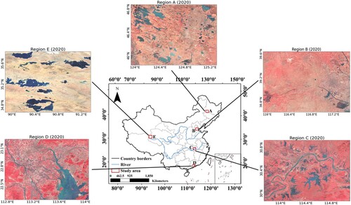
The distribution of surface water in China is characterized as extremely uneven and highly dynamic (Zhang et al. 2020). Therefore, to assess the robustness of the proposed method, we selected five typical sites in China with varied climate, topography, and urbanization conditions (Regions A–E, in Figure 1). Regions A and B are located in northern China, where the precipitation is much less than in the humid southern regions. As a result, the surface water resources are relatively sparsely distributed in these regions. Region C is part of the Wuhan urban agglomeration located in the middle reaches of the Yangtze River, where abundant lakes and drainage systems are found. Region D lies near the Pearl River estuary and belongs to the Pearl River Delta urban agglomeration. Both Regions C and D represent the southern regions in China, with abundant water resources, dense artificial land surfaces, and high precipitation in the wet seasons (i.e. spring and summer). Comparatively, Region E lies in the northern part of the Tibetan Plateau, with low population, where the changes of the water resources are mainly due to climate change. In this area, there are several large lakes that are distinct from the neighboring land areas. However, this high-altitude area is frequently covered by cloud, which brings difficulty to the accurate mapping of long-term surface water dynamics. Some detailed information about the study sites is presented in Table S1.

Figure 1. Overview of the five study sites in China.

2.2. Data

2.2.1. Landsat archives

In this study, we incorporated the Landsat 5 Thematic Mapper (TM), Landsat 7 Enhanced Thematic Mapper Plus (ETM+), and Landsat 8 Operational Land Imager (OLI) surface reflectance products from 1 January 1999 to 31 December 2020 covering the five study sites. All the available image scenes were used for the surface water mapping and occurrence statistics, regardless of the contamination by cloud, shadow, and data voids. The use of the contaminated images can increase the potential information for water mapping (Yao et al. 2019), while the processing of the contaminated pixels was further implemented with quality assessment (Section 3.1) and a temporal correction algorithm (Section 3.4). All the data were accessed and processed using the GEE platform.

2.2.2. GSWD and GLAD products

Two comprehensive global surface products were used in this study to extract the training samples and act as reference data for the temporal correction of the contaminated information. The GSWD product is a 30-m spatial resolution global surface water dataset released by the Joint Research Centre (JRC) (Pekel et al. 2016). The product records the spatial and temporal distribution of surface water from 1984 to 2020. In this study, we used the surface water occurrence (SWO), yearly water history (YWH) datasets and monthly water history (MWH) from GSWD. The SWO dataset gives the long-term frequency of where water was present on the Earth’s surface from March 1984 to December 2020, with the values ranging from 0 to 100. The YWH dataset provides information on the intra-annual seasonality of water areas over the past 3.7 decades, where the pixels over the globe are classified as no observations, not water, seasonal water, and permanent water, based on the monthly water maps throughout the year. The MWH dataset records water detection results at monthly scales, and each pixel is classified as invalid, non-water or water, respectively.

Recently, the GLAD laboratory released a new 30-m global surface water dataset (i.e. the GLAD product) (Pickens et al. 2020). This dataset was generated from all the Landsat 5, 7, and 8 images acquired from 1999 to 2021. The annual water percent (AWP) dataset from GLAD was used in our study, which provides the percentage of water presence for the valid observations to represent the intra-annual variation of water extent throughout a year. For this dataset, the ratio of $\mathrm{water}/(\mathrm{water}+\mathrm{land})$ per season was first counted with the number of valid observations, and the average of the seasons with enough data was used to obtain the AWP.

2.2.3. Manually labeled samples

Manually collected samples were used to assess the accuracy of the obtained classification results. The reference water and non-water samples for the validation were produced from the Landsat monthly image archives at an annual scale in 2000, 2005, 2010, 2015, and 2020, respectively. The five-year maximum water maps of GSWD-YWH are merged to obtain the union set, and determine the extent of water and non-water stratums. Specifically, the image with the lowest cloud cover was selected, and the water and non-water pixels were then visually identified from the valid pixels (i.e. those pixels with no cloud or shadow cover) using high-resolution Google Earth imagery as auxiliary information. If all the images in one month were covered with a high percentage (>70%) of cloud, the images were abandoned. At each year scale, 1000 control points were collected for each study region, where the sample sizes allocated to water and non-water stratums were approximately proportional to the area of each category calculated based on water and non-water stratums defined. In the cases where area proportion of water was less than 10% (e.g. Region B), the sample size for water class was set as 10% of the total number. The specific information about the sample allocation was presented in Table S2.

In total, 5000 manually labeled samples were collected for the independent validation for each study site. The reference samples were distributed all over the study sites (see Figure 5), covering permanent water pixels located in the central parts of large lakes and reservoirs, seasonal water pixels distributed along the borders of water bodies, and non-water pixels belonging to different land-cover types. In Table S2, we also showed the seasonal characteristics of water samples, where the extent of permanent and seasonal water area was determined based on the GSWD-YWH data.

3. Method

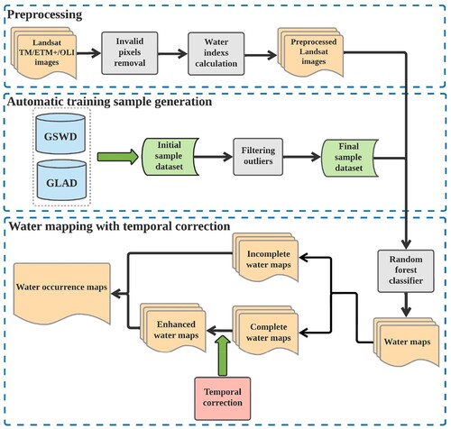
The automatic processing flow for the surface water mapping in this study was shown in Figure 2. Firstly, the available images were preprocessed with the invalid pixels masked (Section 3.1). The water and non-water samples were then automatically selected from the image archives, integrating information from the GSWD and GLAD water occurrence datasets, to construct the training sets (Section 3.2). The masked images and the labeled training samples were used to train the RF classifier for surface water extraction in a supervised manner (Section 3.3). To deal with the potential invalid pixels, the per-scene classification results obtained by the trained RF model were repaired based on the temporal information inferred from the GSWD-SWO statistics (Sections 3.4). The water occurrence maps can be then derived (Section 3.5).

Figure 2. Flowchart of the automatic surface water mapping framework.

3.1. Data preprocessing

The surface reflectance products from the Landsat 5, 7, and 8 satellites were used in this study, which have been processed with radiometric calibration, atmospheric and geometric correction. The extra necessary processing for the images included masking of the low-quality observations, e.g. the pixels contaminated by cloud, cloud shadow, snow/ice, and terrain shadow. Firstly, the Quality Assessment band of each Landsat image was used to identify the poor-quality observations (Zhu, Wang, and Woodcock 2015). To reduce the effects of topographic shadows with a similar low reflectance to water pixels, the topographic shadows were further masked using the SRTM DEM V3, along with the azimuth and zenith angles for each scene (Zou et al. 2018). This was implemented using the ee.Terrain.hillShadow tool on the GEE platform. All the detected low-quality pixels were masked as invalid values, which were excluded from the subsequent training sample construction and water detection process.

3.2. Automatic training sample construction

The key issue for accurate surface water mapping is to construct representative training samples composed of labeled water and non-water pixels. However, this is a challenging task, due to the heterogenous spectral characteristics of water bodies. To capture sufficient water samples with diverse reflection spectra, it is necessary to extract samples from multi-temporal images, due to the highly dynamic nature of water areas. As the detection errors for mapping seasonal water mainly influence the accuracy, the samples should cover both permanent and seasonal water pixels. With the successive release of water datasets, there is now a chance to automatically extract training sample sets from the existing water maps. Nevertheless, the accuracy of the water mapping results for the water products differs with the different data and processing flows employed. Based on these facts, we propose a robust scheme for the automatic construction of training samples by integrating information from multiple water mapping datasets in this study, as shown in Figure 3.

Figure 3. Automatic construction of training samples based on the multiple water occurrence products.

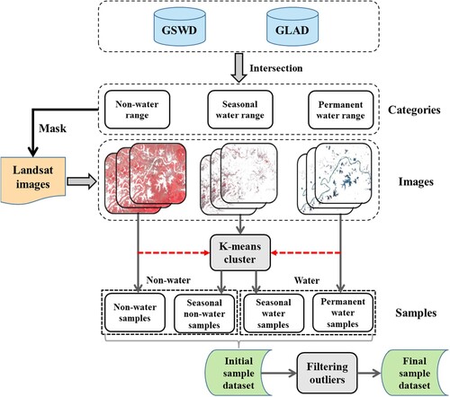
Firstly, an initial training sample set was generated by merging the corresponding classes provided by the GSWD-YWH and GLAD-AWP datasets to obtain the extent of three water types, i.e. permanent water, seasonal water, and non-water. Before this, the water percent values of the GLAD-AWP dataset needed to be converted to labels of water types that were consistent with the GSWD-YWH dataset. We adopted the thresholds to distinguish the annual water occurrence (denoted as $Fw$ hereafter) into permanent water ($Fw\ge 0.75$), seasonal water ($0.25\le Fw<0.75$), and non-water ($Fw<0.25$) areas (Zou et al. 2017). It should be noted that the criteria used to define the seasonal characteristics are different for the GSWD and GLAD datasets. This is because the JRC use the monthly composite water map to generate the GSWD-YWH dataset, where seasonal water is defined as being covered by water for 1–11 months of the year. In contrast, the GLAD-AWP dataset denotes the seasonally normalized percentage of water observations among all the clear observations each year. The statistics are difficult to be treated identically due to their different temporal scales. However, our aim here is to determine a pixel set where high-accuracy training samples can be selected from, rather than extracting the complete extent of water dynamics. Therefore, the intersection of these two datasets corresponding to the three water types were generated as the source of training samples. This meant that the pixels could be indicated as being potential samples of permanent water/non-water only if the pixels were identified as permanent water/non-water for both the GSWD-YWH and GLAD-AWP datasets. In this way, samples for permanent water and non-water could be generated with random selection from the yearly image sets masked by the combination map. About 500 potentially permanent water and 3000 non-water pixels were randomly selected for each year, and the initial training datasets were constructed at a five-year interval for 1999–2020.

For the seasonal water, the yearly merged masks were overlaid on the collected image archives for each year. For each year, 500 multi-temporal samples were then randomly selected from the masked seasonal water areas. Due to the seasonal dynamics, these samples needed to be classified as either water or non-water pixels depending on the specific spectral shape. Therefore, we used a k-means clustering algorithm constrained by the preliminary sample sets for the permanent water and non-water areas, to classify the seasonal samples. It means that the clustering centers for k-means algorithm were initialized by the samples for the permanent water and non-water types, respectively. In this way, the seasonal samples were finally clustered into water and non-water categories, based on the spectral similarities. To ensure the accuracy of the sample sets, the k-means clustering algorithm was again applied to the whole sample set, and two clusters (i.e. water and non-water type) were obtained with randomly assigned initial clustering centers. The results obtained in these two different ways were compared with each other, and the points with inconsistent categories were labeled as potential outliers. The outliers were then removed, and the final sample set was generated. The goal of clustering process is to incorporate an additional proportion of potentially seasonal water samples with diverse spectral properties of surface water in the model training process.

3.3. Water detection with the random forest classifier

The extraction of the surface water area from the remote sensing images was implemented in a supervised manner, with RF employed as the classifier. As a popular statistical classifier, RF has been widely used for surface water mapping and change monitoring, and has showed stable performances (Li and Xu 2021; Rodriguez-Galiano et al. 2012; Tulbure et al. 2016). RF is an integrated predictor that builds a set of decision trees, which can effectively reduce the single model’s sensitivity to data noise and anomalies (Breiman 2001).

To better separate the spectral characteristics, 13 variables related to spectral properties of water and vegetation cover were selected as feature bands for training the RF classifier in this study: six spectral bands (blue, green, red, NIR, SWIR-1, SWIR-2) and seven spectral indices (Table S3) (i.e. Normalized Difference Water Index (NDWI) (McFeeters 1996), Modified Normalized Difference Water Index (mNDWI) (H. Xu 2006), Automatic Water Extraction Index (AWEI) (Feyisa et al. 2014), Enhanced Water Index (EWI) (Yan, Zhang, and Zhang 2007), City Water Index (CWI) (Yang et al. 2018), Normalized Difference Vegetation Index (NDVI) (Tucker 1979) and Enhanced Vegetation Index (EVI)) (Huete et al. 1997; Huete et al. 2002). The input sets to the RF model were made up of all the feature variables, and the model was trained with the automatically constructed samples as the labels. The well-trained RF model was then used to classify each Landsat image. With the fully automatic processing flow of the sample reconstruction, the classifier can be flexibly trained on either a regional or global scale. In this study, we performed the training and testing process for each region (approximately 1° × 1° tile). The number of trees for RF model was set as 150 empirically.

3.4. Temporal correction of contaminated pixels

Optical remote sensing images are often contaminated by cloud, cloud shadow, and topographic shadow. Most studies discard the contaminated images or pixels, but this can lead to bias in the analysis of the spatial and temporal distribution of surface water resources (Pekel et al. 2016; Pickens et al. 2020; Zou et al. 2018). Moreover, the different methods employed for the detection and processing of invalid pixels cause inconsistency among the various water products. Following the idea of Zhao and Gao (2018), we optimized the water mapping results through correction of the contaminated pixels based on the water occurrence statistics. Instead of processing the monthly water coverage for the reservoirs from the GSWD product, we applied the correction method to repair the scene-based classification results.

To extract the water extent, the collected images were first classified into three categories, i.e. water, non-water, and invalid observations. For each scene, the invalid pixels were then reclassified as water or non-water types, based on the temporal clues. The general idea behind the method of Zhao and Gao (2018) is to introduce the long-term water occurrence information to infer the category of the contaminated pixels. In this study, we employed the GSWD-SWO data to provide the water occurrence information during the 37-year period (1984–2020). The basic assumption was that the contaminated pixels were likely covered by water when their water occurrence values $O_{ci}$ were greater than the occurrence threshold determined by the uncontaminated water pixels within the data tile. Specifically, the GSWD-SWO data were cropped using the mask generated by the classified water area for each image, and the histogram of the cropped occurrence image was generated. The histogram shows the count of pixels corresponding to each water occurrence value. The average value of the pixel counts ($P_{wc}$) for regional water area was then calculated, and the count threshold ($T_{wc}$) was set as the product of $P_{wc}$ and a weighting factor ($\alpha =0.17$), following the instructions provided in Zhao and Gao (2018). After the count threshold was determined, the occurrence threshold ($T_{wo}$) could then be identified as the smallest water occurrence with pixel count larger or equal to $T_{wc}$. As a result, the invalid pixels with a water occurrence greater than the threshold were identified as water ($O_i\ge T_{wo}$); otherwise, the pixels were reclassified as the non-water category. Finally, an enhanced classification image was produced after temporal correction of the invalid pixels.

For some cases without enough valid observations in a scene, the method can fail due to the inaccurate threshold obtained. Therefore, if the estimated occurrence threshold is out of the range of 5–75%, the correction process was not applied to the classification results for the purpose of quality control. Moreover, for the images with good quality (more than 95% valid observations) and extreme contamination (less than 5% valid observations), the correction processing was meaningless.

3.5. Calculation of water occurrence

Water occurrence represents the occurrence of surface water for a pixel within a given period. The water occurrence can be obtained from the multi-temporal classified water body maps, and denotes the ratio of the number of pixels identified as water to the total number of observations. For the scenes with correction of contaminated pixels, they are counted into the sum of the total observations. Based on the water occurrence values, the pixels were then classified into permanent water ($Fw\ge 0.75$), seasonal water ($0.25\le Fw<0.75$), and non-water ($Fw<0.25$) categories in this study.

3.6. Accuracy evaluation

In the validation stage, the accuracy of the automatically collected samples and the accuracy of the water classification results were evaluated based on the corresponding validation sets. The accuracies of both the samples and overall classification were calculated based on confusion matrices with cell entries expressed in terms of area proportions (Olofsson et al. 2014; Stehman and Foody 2019). The derived accuracy indices included the area-weighted overall accuracy (OA), user’s accuracy (UA), producer’s accuracy (PA), where the expressions for calculation can be found in the supplementary material (Tables S4 and S5). In addition, accuracy evaluation was conducted for the water samples (both permanent and seasonal water samples presented in Table S2) to characterize errors of commission judged by seasonal class.

The validation strategies were different for evaluating the mapping results and training samples. In terms of evaluating the water mapping results, the independent manually labeled sample sets were used (Section 2.2.3), where proportional allocation was employed. For the evaluation of the samples at each study site, we used a stratified sampling strategy to randomly select a total number of 250 sample points from the total training samples within the permanent water, seasonal water, and non-water strata for each year of 1999, 2004, 2009, 2014, and 2009. Strata were created for the three classes derived from annual water occurrence (the combination map integrating GSWD-YWH and GLAD-AWP used here, as similar as in Section 3.2). The annually selected samples were composed of 100 non-water points, 100 permanent water points, and 50 seasonal points (either non-water or water types), and the five-year data were made up of all the sample sets for the validation. Although proportional allocation can result in smaller standard errors for estimating the OA values (Olofsson et al. 2014; Stehman and Foody 2019), the precision of water samples was vital for deriving a reliable classifier for water mapping. Therefore, we increased the proportion of water pixels in the sample sets for validation. To explore the temporal characteristics of the samples, the points to be validated were selected across the monthly image archives throughout the year. The selected sample sets were manually interpreted by visual examination, considering the pixels’ spatial and spectral characteristics. The images covered with more than 50% invalid pixels were discarded to ensure the selected samples can be interpreted.

In addition to the quantitative evaluation, the water mapping results are also compared with the results obtained by the commonly used water indices, as well as with the GSWD and GLAD datasets, via visual analysis.

4. Results

4.1. Accuracy evaluation of the automatically constructed training samples

To validate the accuracy of the training samples, 250 randomly selected training samples collected in 1999, 2004, 2009, 2014, and 2019 within Regions A–E are visually examined. The spatial distribution of the sampling points for validation and the associated errors for the five study regions in 2019 is shown in Figure 4. The confusion matrix is given in Table 1, where the OA is used to quantify the evaluation results.

Figure 4. The spatial distribution of the sample points for validation and errors within Regions A–E (2019).

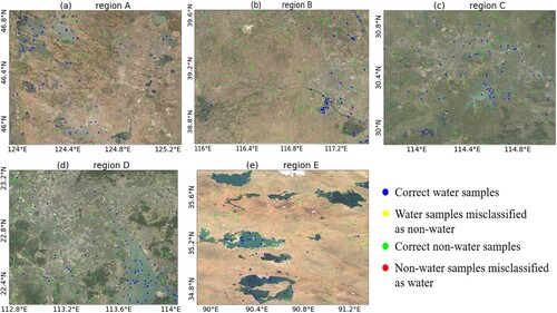
Table 1. The error matrix of the training sample set in the study areas.

Region		1999			2004			2009			2014			2019			Total
		NW*	W*	OA	NW*	W*	OA	NW*	W*	OA	NW*	W*	OA	NW*	W*	OA	OA
A	NW	122	3	98.4%	135	0	99.1%	122	1	98.8%	132	3	98.5%	124	2	98.8%	98.7%
	W	1	124		2	133		2	125		1	114		1	123
B	NW	117	0	98.9%	100	0	99.3%	116	1	99.2%	123	2	98.8%	122	2	98.8%	99.0%
	W	3	130		2	148		1	132		1	124		1	125
C	NW	125	1	98.8%	137	2	99.3%	127	1	98.4%	135	2	98.4%	118	4	98.0%	98.6%
	W	2	122		0	111		3	119		2	111		1	127
D	NW	115	3	98.3%	132	1	98.8%	128	2	98.8%	136	5	98.2%	129	5	98.1%	98.4%
	W	1	131		2	115		1	119		0	109		0	116
E	NW	124	2	98.8%	128	0	99.2%	133	3	98.9%	118	2	99.2%	120	2	98.8%	99.0%
	W	1	123		2	120		0	114		0	130		1	127
Overall	/	/	/	98.6%	/	/	99.1%	/	/	98.8%	/	/	98.6%	/	/	98.5%	98.7%

* NW: predicted non-water; W: predicted water; NW*: labeled non-water; W*: labeled water.

Cell entries are presented in terms of the number of samples, and the derived accuracy indices are calculated in terms of proportion of area in Tables S4 and S5.

The validation results show that the OA for the training sample sets is 98.7%, over all the study sites. Region B and Region E achieve the equally high precision (OA: 99.0%). For Region B, the high precision is likely because surface water is relatively sparse in the northern part of China. In terms of Region E, the water bodies in this region are mainly large lakes with clear boundaries. Comparatively, the accuracy of the sample sets in Region A (OA: 98.7%), Region C (OA: 98.6%) and Region D (OA: 98.4%) is relatively lower. This is mainly because the water types in these urban regions are complicated and contain large numbers of urban targets that are difficult to recognize. Similar trends can be found in analyzing the precision of water and non-water samples, which can be derived with the cell entries in Table 1. Moreover, as shown in Figure 4, the yellow and red dots indicate the spatial distribution of water samples with omission and commission errors in 2019, respectively. The results show that errors mainly occur in the minor water bodies, and along the border of rivers and lakes. However, the number of those incorrectly classified samples is small, which demonstrate that the automatically constructed training sample sets are of high quality and can be considered as reliable for the subsequent surface water mapping. Considering the variations of the spectral properties of water, the automatically constructed training samples were composed of both permanent water/non-water samples and seasonal samples. To interpret the distribution of the training samples in the spectral feature space, please refer to Figure S1. Given that the amount of incorrectly classified water samples is rather small, we did not calculate extra accuracy indexes judged by seasonal class.

4.2. Accuracy assessment of the water mapping results

4.2.1. Accuracy of the surface water maps

In this section, we evaluate the surface water mapping results using the manually labeled samples as the reference. Each annual sample set for 2000, 2005, 2010, 2015, and 2020 contained 1000 water and non-water pixels, where the number of samples for each category can be found in Table S2. As an example, the spatial distribution of the sample points and the associated errors within Regions A–E in 2020 is presented in Figure 5. The area-weighted UA, PA, and OA values calculated using the samples and water mapping results for the corresponding images are shown in Table 2. Furthermore, the accuracy results for permanent and seasonal water are given in Table 3.

Figure 5. Spatial distribution of the manually labeled sample points and errors within Regions A–E (2020).

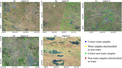
Table 2. Area-weighted accuracy of water mapping classification results based on the validation sets in the study areas (NW: non-water; W: water).

Region		2000			2005		2010				2015			2020			Total
		UA	PA	OA	UA	PA	OA	UA	PA	OA	UA	PA	OA	UA	PA	OA	OA
A	NW	99.6%	99.0%	98.9%	100%	98.1%	98.5%	99.9%	98.4%	98.7%	99.6%	99.1%	99.0%	99.9%	98.4%	98.6%	98.7%
	W	96.4%	98.6%		93.2%	100%		94.4%	99.5%		96.9%	98.6%		93.4%	99.5%
B	NW	99.9%	99.2%	99.2%	99.8%	98.9%	98.8%	99.6%	98.8%	98.5%	99.2%	99.0%	98.4%	99.7%	99.4%	99.1%	98.8%
	W	92.5%	98.9%		89.9%	97.8%		88.9%	95.7%		91.2%	92.9%		94.2%	97.0%
C	NW	97.8%	99.4%	97.9%	97.8%	99.9%	98.2%	99.2%	98.7%	98.4%	99.3%	98.2%	98.2%	99.3%	98.7%	98.5%	98.2%
	W	98.3%	93.6%		99.6%	93.7%		96.1%	97.5%		94.6%	97.9%		96.1%	97.9%
D	NW	98.8%	99.7%	98.9%	99.1%	98.8%	98.4%	99.0%	99.3%	98.8%	98.1%	99.6%	98.3%	98.0%	99.6%	98.2%	98.5%
	W	99.2%	96.8%		96.7%	97.4%		98.1%	97.4%		98.8%	95.1%		98.8%	94.8%
E	NW	99.8%	99.5%	99.4%	99.9%	99.6%	99.6%	99.8%	99.3%	99.2%	99.9%	99.6%	99.6%	99.8%	99.6%	99.5%	99.5%
	W	97.5%	98.7%		98.1%	99.4%		96.3%	98.7%		98.1%	99.4%		98.1%	98.7%
Overall	NW	99.2%	99.3%	98.8%	99.3%	99.0%	98.7%	99.5%	98.9%	98.7%	99.2%	99.1%	98.7%	99.3%	99.1%	98.8%	98.5%
	W	97.4%	96.8%		96.1%	97.3%		95.5%	97.9%		96.4%	97.0%		96.4%	97.4%

The derived accuracy indices are calculated in terms of proportion of area in Table S2.

Table 3. Accuracy for seasonal and permanent water samples among the validation sets in the study areas.

Region	Water types	Misclassified as non-water	Correctly classified as water	Product’s accuracy
Region A	Seasonal water	4	104	96.3%
	Permanent water	0	981	100%
	Overall water	4	1085	99.6%
Region B	Seasonal water	7	241	97.2%
	Permanent water	0	240	100%
	Overall water	7	481	98.6%
Region C	Seasonal water	21	206	90.7%
	Permanent water	1	975	99.9%
	Overall water	22	1181	98.2%
Region D	Seasonal water	17	148	89.7%
	Permanent water	2	1113	99.8%
	Overall water	19	1261	98.5%
Region E	Seasonal water	1	36	97.3%
	Permanent water	5	754	99.4%
	Overall water	6	790	99.2%
Total	Seasonal water	50	735	93.6%
	Permanent water	8	4063	99.8%
	Overall water	58	4798	98.8%

The seasonality of pixels was determined based on the GSWD-YWH data.

The average OA of the surface water maps for the five study areas is 98.5%, which indicates that the mapping results have been validated to be of high accuracy using the 25,000 random samples distributed across spatial and temporal scales. Specifically, the non-water category generally has a higher UA and PA than the water class. Moreover, the accuracy of the water maps varies for the different regions. Region E has the highest accuracy (OA: 99.5%), which is consistent with the accuracy evaluation results for the sample sets in Table 1. As for Regions C and D, the accuracies are relatively lower. The complex drainage systems within those two humid urban regions might be the main reason for this result. For Regions A and B, we noticed that the PA values are higher than the UAs for the water class, which indicate that the commission errors are the major factors influencing the overall accuracies. The distribution of erroneous points presented in Figure 5 also agree well with the quantitative accuracy evaluation results. In terms of the accuracies judged by seasonality class given in Table 3, the accuracy of permanent water mapping (average PA: 99.8%) is higher than that of seasonal water (average PA: 93.6%). Among the study regions, Region E has the highest accuracy of extracting seasonal water pixels (PA: 97.3%), and Region D (PA: 89.7%) has the lowest accuracy.

Although the accuracy of the surface maps differs slightly between the study sites, the results indicate that the proposed method shows a robust performance in surface water mapping with the training sample sets automatically constructed at a regional scale.

4.2.2. Comparison with water indices

Three commonly used water indices (i.e. NDWI, mNDWI, AWEI) were selected for the comparison. For a fair comparison, the optimal thresholds for the three index-based algorithms were manually adjusted for each region. We did not use the commonly used Otsu’s thresholding method to automatically determine the thresholds because it failed to obtain satisfactory results, possibly due to the large-scale and complex land-cover distribution in our cases. The water mapping results for the image scenes across the five study sites are presented in Figures 6 and 7.

Figure 6. Comparative performance in water mapping. The first column is the raw image, and the successive columns indicate the results obtained by the proposed method and the NDWI, mNDWI, and AWEI indices, respectively. The rows from top to bottom represent the results for Regions A–E. $T$ is the manually adjusted threshold for the water indices. The clouds are masked as white pixels. Zoomed-in views of the corresponding highlighted regions marked by the rectangular boxes are presented in Figure 7.

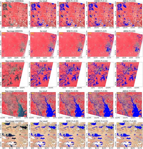
Figure 7. Zoomed-in views of the corresponding highlighted rectangular regions in Figure 6. The regions with distinctive performance in the figures are highlighted with the rectangular boxes.

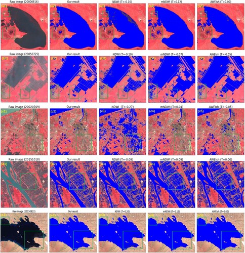
Among the four methods, the NDWI algorithm obtains the worst results, where a substantial number of non-water pixels are misclassified as water, and the complete shape of the water bodies is frequently omitted. The commission errors mainly come from the man-made targets in the urban areas with confusable spectral features in the visible bands, which can be clearly observed in Figures 6 and 7(c). Comparatively, the other three methods obtain similar mapping results. All the methods are influenced by the shadow and dark targets, to different extents. However, the mNDWI and AWEI indices tend to produce more noisy outputs, as shown in the highlighted regions in Figure 7(b) and (c). Furthermore, both the mNDWI and AWEI can hardly distinguish accurate boundaries among the small ponds and paddy fields, which are commonly found in the southern part of China (as shown in Figure 7(d)). With the distinctive spectral reflectance of clear water and few building shadows, the results for Region E (Figures 6 and 7(e)) show the best accuracy, with only marginal differences between the classification methods. Overall, the proposed method obtains promising water mapping results in all the cases, and can extract the seasonal water pixels along the borders of water bodies well. Through the tests conducted for the five study sites with varied land-cover patterns, terrain conditions, and image qualities, the proposed water mapping method showed a robust performance in large-scale water mapping. Furthermore, the fully automatic processing pipeline is superior to the other index-based methods as no extra manual labor is required.

4.2.3. Comparison with the existing global water datasets

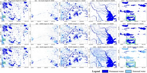
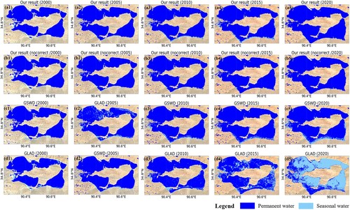
In this section, we compare the annual water occurrence derived by the proposed method with the existing GSWD and GLAD products. Figure 8 presents the permanent and seasonal water mapping results for 2020 for the different water datasets. For the results obtained by the proposed method and the GLAD dataset, the permanent and seasonal water was classified according to the annual water percentage in 2020, based on the thresholds defined in Section 3.5. For the GSWD product, the mapping results were derived from the published YWH dataset. Overall, the results confirm that the results of the proposed method are generally consistent with the GSWD product. Comparatively, the GLAD product tends to contain more noisy results due to the large amounts of misclassified pixels (Figure 8(d) and (e)). Moreover, the water maps and statistics for the GLAD product show quite different distributions, compared with the other two datasets, especially for Regions D and E.

Figure 8. The permanent and seasonal water mapping results derived from the water occurrence for 2020 for the different water datasets in the five study sites. From top to bottom, each row indicates the results for the proposed method, GSWD, and GLAD, respectively. Moreover, columns (a)–(e) show the corresponding results for Regions A–E.

In Figures 9 and 10, the zoomed-in visual inspection for the highlighted subregions in Figure 8 provides more detailed information, where the annual water mapping results for 2000–2020 at a five-year interval are provided for comparison. In Figure 9, the GSWD product fails to extract the complete boundary of the small-size lake, with the central regions within the lake polygon categorized as seasonal water. This is likely caused by the terms used for distinguishing annual seasonal water by the GSWD product, in that a pixel would be excluded from the permanent water category if it was classified as a non-water type in any one of the valid monthly water maps. In this way, the water mapping results can be sensitive to the accuracy of the monthly composite imagery and the derived classification results. Figure 10 shows another featured case, where the water mapping results for Lake Ulan Ula in Qinghai, China, are presented. This is a natural salt lake with marshlands distributed along the lakeshore, where the lake surface can be frozen for as long as six months within a year. In this case, there are enormous differences in the water area statistics between the GLAD product and the other two datasets (Figure 8(e)). Similar to the processing flow of the GSWD product, the GLAD product regards the ice and snow-covered water area as invalid pixels and excludes them from the calculation of the water occurrence. However, a large area of ice-covered water is wrongly classified as non-water pixels in the monthly water map for 2020 (Figure S2). As a result, the water occurrence is underestimated, and this large area of permanent water is wrongly classified as seasonal water. The GSWD product’s monthly water maps are also presented in Figure S3. There is obvious inconsistency between the two open-access datasets, which is probably caused by the different detection algorithms for water and invalid pixels. Compared with the GLAD and GSWD products, the proposed method calculates the water occurrence based on the images throughout a year. Moreover, some of the contaminated information can be repaired through the temporal correction of invalid pixels, producing more robust water mapping results. The temporal correction causes various degrees of change in different areas, as shown in Figures 9 and 10. More details about the effectiveness of the temporal correction are provided in Section 5.2.

Figure 9. Annual water mapping results for the highlighted region in Figure 8(a). The second row indicates the results obtained by the proposed method without temporal correction.

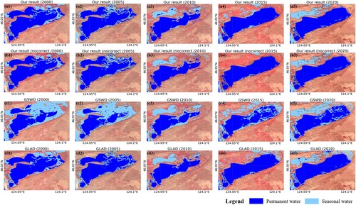
Figure 10. Annual water mapping results for the highlighted region in Figure 8(e). The second row indicates the results obtained by the proposed method without temporal correction.

5. Discussions

5.1. Commission and omission error sources

The experiments presented in Section 4 showed that the proposed method achieved generally good results in the five study sites with varied hydrological conditions. However, some potential limitations should be considered. It was found that shadow pixels are one of the commission error sources for water detection in urban areas and rugged terrain regions. With the similar low reflected spectral signals for the visible and infrared bands, shadow pixels are easily misclassified as water (Figure 7(b) and (c)). For the areas with rugged terrain, the incorporation of DEM data can exclude most of the topographic shadows from the extracted water areas. However, the accurate identification of building shadows is still challenging. Visual inspection of Figure 7(c) shows that the proposed method suppresses the urban shadowed areas effectively, and results in smaller commission errors than the water indices. This can be attributed to the proposed method benefiting from the diverse spectral features contained in the randomly selected sample sets covering various land types in the training process.

Moreover, the pixels distributed near the edge of water bodies are often characterized by mixed spectral features from both water and land, making them difficult to be accurately recognized (Huang et al. 2018; Li and Xu 2021). By incorporating seasonal water samples in the training set, which typically reflect the diverse spectral properties of shallow water pixels, the proposed method performs better in extracting the complete boundaries of water bodies. However, the spatial resolution of Landsat images is only 30 m, and thus some narrow channels and edge pixels with a small fraction of water among the mixed pixels can still be missed. This is reflected in the results where some drainage and lake polygons are discontinuous (e.g. Figure 7(b) and (d)). In this study, we did not pay much attention to sub-pixel accuracy assessment for the edge pixels. This was since it is difficult to define whether a mixed pixel should be classified as water or non-water without prior knowledge of the accurate sub-pixel water percentage. This information can be acquired with the aid of high-resolution images, but the precise registration between 30-m Landsat images and meter-level images is challenging. Therefore, we focused on the pixel-level accuracy assessment for the water mapping task.

5.2. Effectiveness of the temporal correction

As shown in Figure 11, the temporal correction process effectively reconstructs the missing information and generates seamless water maps. However, the results also indicate that the improvement differs between regions. Thus, how can we confirm the efficacy of the temporal correction process? Furthermore, as the long-term water occurrence (1984–2020) was used as the reference for the correction (Section 3.4), how would the result be affected with a different reference employed?

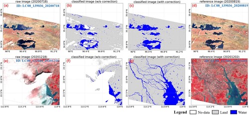
Figure 11. Water mapping results before and after temporal correction. The first column is the raw imagery, and the second column is the preliminary classification results of the random forest classifier. The third column is the mapping results after temporal correction for invalid pixels, while the last column is the reference image without cloud cover.

In Table 4, we present the statistics for the number of images in the sampling years for each study site. The results show that the ratio of corrected images (RCI) is only 2.03% for Region B. Comparatively, the RCI for Region E is as high as 83.50%. This means that, among the 394 images used to calculate the water occurrence for Region E in these five years, only 16.5% of them (65 scenes) were good-quality images (cloud cover less than 5%) that did not need correction. Combined with the number of abandoned low-quality images, only 0.79% of the contaminated images ($NCI/(NCI+NUI)$) were corrected for Region B, while the corresponding proportion was 34.9% for Region E. The low proportion of corrected images for Region B is mainly due to the relatively sparse distribution of surface water in this area. If there was not enough water area to derive a statistically significant occurrence histogram, the correction process would be terminated as the occurrence threshold would be out of the range of 5–75% (see Section 3.4). For Region E, this area is characterized by low precipitation, and thus the cloud coverage is also relatively low. However, as the high-latitude lakes are frozen for much of the year, there are still a large number of contaminated images to be corrected. The waterbodies in Region E are mainly composed of large- and medium-size lakes. Therefore, the temporal correction method shows an excellent performance in repairing the contaminated scenes in this region. For Regions C and D with more humid climate conditions, the ratio of images with extreme cloud pollution is high, which were hardly effectively corrected. Overall, the temporal correction is effective in cases where sufficient water information is available to infer the regional water distribution. The temporal correction shows a robust performance for the partly contaminated images, and significantly improves the number of effective images for the temporal analysis.

Table 4. Statistics on the number of images for each study site.

Region	2000			2005			2010			2015			2020			RCI
	NGI	NCI	NUI	NGI	NCI	NUI	NGI	NCI	NUI	NGI	NCI	NUI	NGI	NCI	NUI
A	31	30	152	29	29	113	43	21	110	35	44	113	26	3	136	52.92%
B	74	2	203	79	3	191	68	1	174	78	2	221	87	0	219	2.03%
C	18	4	66	17	10	66	18	3	66	25	15	95	24	2	83	25.00%
D	19	20	121	13	13	109	17	16	73	24	15	138	11	23	137	50.88%
E	5	11	133	6	44	119	6	90	90	17	136	123	31	48	196	83.50%

NGI denotes the number of good-quality images, and NCI represents the number of corrected images. RCI is the ratio of corrected images, where $\mathrm{RCI}=\mathrm{NCI}/(\mathrm{NCI}+\mathrm{NGI})$. NUI represents the number of unused images which were abandoned due to low quality.

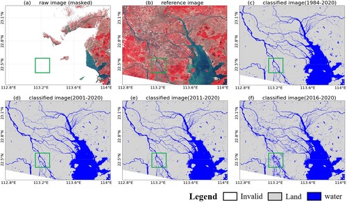
Taking Figures 12 and 13 as examples, we evaluated the effectiveness of the temporal correction by analyzing the scene-based correction results, and tested the impact of the temporal scale of the water occurrence data used as a reference. The GSWD-SWO data corresponding to four different temporal windows were tested, i.e. 1984–2020, 2001–2020, 2011–2020, and 2016–2020. The results indicate that, for some large lakes occupied by permanent water, the correction process is generally satisfactory, regardless of the reference used. In this case, the long-term occurrence information can help to prevent the results being contaminated by noise, as shown in Figure S4. However, surface water is highly dynamic, especially in the context of global warming and accelerated urbanization. For the water areas with abrupt changes in recent years, such as the expanded lakes and newly built reservoirs, a derived water occurrence close to the acquisition time of the imagery can better reflect the real distribution of the water. This can be observed in Figure 13 and Figure S5, where the paddy fields and aquaculture area occurring after 2010 are easily missed based on the long-term water occurrence. Based on these results, we suggest using five-year or ten-year composite water occurrence data for the temporal correction in the regions with recent changes. For some highly dynamic regions, short-period water occurrence data close to the image acquisition time should be used as the reference.

Figure 12. Water mapping results for Region E after temporal correction referenced by water occurrence data with different temporal scales. (a) The raw image for interpretation. (b) The reference image. (c)–(f) The corrected results corresponding to four occurrence datasets with different temporal windows, i.e. 1984–2020, 2001–2020, 2011–2020, and 2016–2020. A zoomed-in view of the highlighted region is shown in Figure S4.

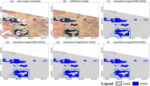
Figure 13. Water mapping results for Region D after temporal correction referenced by water occurrence data with different temporal scales. (a) The raw image for interpretation. (b) The reference image. (c)–(f) The corrected results corresponding to four occurrence datasets with different temporal windows, i.e. 1984–2020, 2001–2020, 2011–2020, and 2016–2020. A zoomed-in view of the highlighted region is shown in Figure S5.

6. Conclusions

In this paper, we have proposed a fully automatic surface water mapping framework on the GEE platform. Firstly, we built a robust scheme to automatically construct training samples by integrating information from the GSWD and GLAD products. Secondly, the classified water maps with invalid observations were repaired using a temporal correction method, obtaining more accurate water occurrence statistics.

The proposed method was employed to produce surface water maps and water occurrence maps and was evaluated in five representative regions in China. The accuracy assessment and visual evaluation indicated that the proposed method could generate good-quality samples (OA: 98.7%), and the accuracy of the mapping results was generally high across the different regions. Comparative tests confirmed that the proposed method can produce better water maps than the index-based water mapping algorithms (including NDWI, mNDWI, and AWEI), as well as the GSWD and GLAD products. The errors mainly come from the shadow areas and pixels distributed along the edge of water bodies with mixed spectral characteristics. Furthermore, the temporal correction is an effective way to increase the valid observations for the temporal analysis. However, attention should be paid to the regions with recent changes, where short-period water occurrence data close to the image acquisition time should be used as the reference. Moreover, seasonal pixels with low water occurrence values might be missed in the reconstruction process. Overall, with the open-access code package, the fully automatic processing pipeline on the GEE platform enables the proposed framework to be used to conduct monitoring and analysis of surface water dynamics at different spatial and temporal scales. We believe that the water datasets derived using the proposed framework can provide extra information for further tasks.

Acknowledgements

We would like to acknowledge Prof. Qiusheng Wu for developing geemap python package, and acknowledge Google for providing free access to the Google Earth Engine platform. We also thank anonymous reviewers and the editors for their constructive comments that helped improve the manuscript.

Disclosure statement

No potential conflict of interest was reported by the author(s).

Data availability statement

The data and Python code package were available to interested users (https://github.com/GISer-Bao/Water-Classification-GEE), where more water mapping results and auxiliary files can be examined.

Additional information

Funding

This work was supported by the National Natural Science Foundation of China [grants numbers 42171375 and 41801263].

References

- Amani, Meisam, Brian Brisco, Majid Afshar, S. Mohammad Mirmazloumi, Sahel Mahdavi, Sayyed Mohammad Javad Mirzadeh, Weimin Huang, and Jean Granger. 2019. “A Generalized Supervised Classification Scheme to Produce Provincial Wetland Inventory Maps: An Application of Google Earth Engine for Big Geo Data Processing.” Big Earth Data 3 (4): 378–394. doi:10.1080/20964471.2019.1690404.
- Breiman, Leo. 2001. “Random Forests.” Machine Learning 45 (1): 5–32. doi:10.1023/A:1010933404324.
- Bukata, Robert P., John H. Jerome, Kirill Ya Kondratyev, and Dimitry V. Pozdnyakov. 2018. Optical Properties and Remote Sensing of Inland and Coastal Waters. CRC Press. doi:10.1201/9780203744956
- Campos, João C., Neftalí Sillero, and José C. Brito. 2012. “Normalized Difference Water Indexes Have Dissimilar Performances in Detecting Seasonal and Permanent Water in the Sahara–Sahel Transition Zone.” Journal of Hydrology 464: 438–446. doi:10.1016/j.jhydrol.2012.07.042.
- Feyisa, Gudina L., Henrik Meilby, Rasmus Fensholt, and Simon R. Proud. 2014. “Automated Water Extraction Index: A New Technique for Surface Water Mapping Using Landsat Imagery.” Remote Sensing of Environment 140: 23–35. doi:10.1016/j.rse.2013.08.029.
- Fisher, Adrian, Neil Flood, and Tim Danaher. 2016. “Comparing Landsat Water Index Methods for Automated Water Classification in Eastern Australia.” Remote Sensing of Environment 175: 167–182. doi:10.1016/j.rse.2015.12.055.
- Gorelick, N., M. Hancher, M. Dixon, S. Ilyushchenko, and R. Moore. 2017. “Google Earth Engine: Planetary-Scale Geospatial Analysis for Everyone.” Remote Sensing of Environment 202. doi:https://doi.org/10.1016/j.rse.2017.06.031.
- Huang, Chang, Yun Chen, Shiqiang Zhang, and Jianping Wu. 2018. “Detecting, Extracting, and Monitoring Surface Water from Space Using Optical Sensors: A Review.” Reviews of Geophysics 56 (2): 333–360. doi:10.1029/2018RG000598.
- Huete, Alfredo, Kamel Didan, Tomoaki Miura, E. Patricia Rodriguez, Xiang Gao, and Laerte G. Ferreira. 2002. “Overview of the Radiometric and Biophysical Performance of the MODIS Vegetation Indices.” Remote Sensing of Environment 83 (1–2): 195–213. doi:10.1016/S0034-4257(02)00096-2.
- Huete, A. R., H. Q. Liu, K. V. Batchily, and W. J. D. A. Van Leeuwen. 1997. “A Comparison of Vegetation Indices Over a Global Set of TM Images for EOS-MODIS.” Remote Sensing of Environment 59 (3): 440–451. doi:10.1016/S0034-4257(96)00112-5.
- Li, Kewei, and Erqi Xu. 2021. “High-Accuracy Continuous Mapping of Surface Water Dynamics Using Automatic Update of Training Samples and Temporal Consistency Modification Based on Google Earth Engine: A Case Study from Huizhou, China.” ISPRS Journal of Photogrammetry and Remote Sensing 179: 66–80. doi:10.1016/j.isprsjprs.2021.07.009.
- Markos, Andrea, Neil Sims, and Gregory Giuliani. 2022. “Beyond the SDG 15.3. 1 Good Practice Guidance 1.0 Using the Google Earth Engine Platform: Developing a Self-Adjusting Algorithm to Detect Significant Changes in Water Use Efficiency and Net Primary Production.” Big Earth Data, 1–22. doi:10.1080/20964471.2022.2076375.
- McFeeters, Stuart K. 1996. “The Use of the Normalized Difference Water Index (NDWI) in the Delineation of Open Water Features.” International Journal of Remote Sensing 17 (7): 1425–1432. doi:10.1080/01431169608948714.
- Mueller, Norman, Adam Lewis, Dale Roberts, Steven Ring, R. Melrose, J. Sixsmith, Leo Lymburner, A. McIntyre, P. Tan, and S. Curnow. 2016. “Water Observations from Space: Mapping Surface Water from 25 Years of Landsat Imagery Across Australia.” Remote Sensing of Environment 174: 341–352. doi:10.1016/j.rse.2015.11.003.
- Olofsson, Pontus, Giles M. Foody, Martin Herold, Stephen V. Stehman, Curtis E. Woodcock, and Michael A. Wulder. 2014. “Good Practices for Estimating Area and Assessing Accuracy of Land Change.” Remote Sensing of Environment 148: 42–57. doi:10.1016/j.rse.2014.02.015.
- Pekel, Jean-François, Andrew Cottam, Noel Gorelick, and Alan S. Belward. 2016. “High-Resolution Mapping of Global Surface Water and Its Long-Term Changes.” Nature 540 (7633): 418–422. doi:10.1038/nature20584.
- Pickens, Amy H., Matthew C. Hansen, Matthew Hancher, Stephen V. Stehman, Alexandra Tyukavina, Peter Potapov, Byron Marroquin, and Zainab Sherani. 2020. “Mapping and Sampling to Characterize Global Inland Water Dynamics From 1999 to 2018 with Full Landsat Time-Series.” Remote Sensing of Environment 243: 111792. doi:10.1016/j.rse.2020.111792.
- Rodriguez-Galiano, Victor Francisco, Bardan Ghimire, John Rogan, Mario Chica-Olmo, and Juan Pedro Rigol-Sanchez. 2012. “An Assessment of the Effectiveness of a Random Forest Classifier for Land-Cover Classification.” ISPRS Journal of Photogrammetry and Remote Sensing 67: 93–104. doi:10.1016/j.isprsjprs.2011.11.002.
- Stehman, Stephen V., and Giles M. Foody. 2019. “Key Issues in Rigorous Accuracy Assessment of Land Cover Products.” Remote Sensing of Environment 231: 111199. doi:10.1016/j.rse.2019.05.018.
- Tucker, Compton J. 1979. “Red and Photographic Infrared Linear Combinations for Monitoring Vegetation.” Remote Sensing of Environment 8 (2): 127–150. doi:10.1016/0034-4257(79)90013-0.
- Tulbure, Mirela G., Mark Broich, Stephen V. Stehman, and Anil Kommareddy. 2016. “Surface Water Extent Dynamics from Three Decades of Seasonally Continuous Landsat Time Series at Subcontinental Scale in a Semi-Arid Region.” Remote Sensing of Environment 178: 142–157. doi:10.1016/j.rse.2016.02.034.
- Vörösmarty, Charles J., Peter B. McIntyre, Mark O. Gessner, David Dudgeon, Alexander Prusevich, Pamela Green, Stanley Glidden, Stuart E. Bunn, Caroline A. Sullivan, and C. Reidy Liermann. 2010. “Global Threats to Human Water Security and River Biodiversity.” Nature 467 (7315): 555–561. doi:10.1038/nature09440.
- Wood, Eric F., Joshua K. Roundy, Tara J. Troy, L. P. H. Van Beek, Marc FP Bierkens, Eleanor Blyth, Ad de Roo, Petra Döll, Mike Ek, and James Famiglietti. 2011. “Hyperresolution Global Land Surface Modeling: Meeting a Grand Challenge for Monitoring Earth’s Terrestrial Water.” Water Resources Research 47 (5), doi:10.1029/2010WR010090.
- Wu, Qiusheng. 2020. “Geemap: A Python Package for Interactive Mapping with Google Earth Engine.” Journal of Open Source Software 5 (51): 2305. doi:10.21105/joss.02305.
- Xu, Hanqiu. 2006. “Modification of Normalised Difference Water Index (NDWI) to Enhance Open Water Features in Remotely Sensed Imagery.” International Journal of Remote Sensing 27 (14): 3025–3033. doi:10.1080/01431160600589179.
- Xu, Yuyue, Xing Cheng, and Zhao Gun. 2022. “What Drive Regional Changes in the Number and Surface Area of Lakes Across the Yangtze River Basin During 2000–2019: Human or Climatic Factors?” Water Resources Research 58 (2): e2021WR030616. doi:10.1029/2021WR030616.
- Yan, Pei, Youjing Zhang, and Yuan Zhang. 2007. “Extraction of Water System Information in Semi-Arid Regions Using Enhanced Water Index (EWI) and GIS de-Noising Techniques.” Remote Sensing Information 6: 62–67. doi:10.3969/j.issn.1000-3177.2007.06.015.
- Yang, Ji, Liusheng Han, Shuishen Chen, and Yong Li. 2018. “A Method for Extracting Water Bodies from OLI Remote Sensing Images Based on Urban Water Body Index and Fractal Geometry Algorithm.” Bulletin of Surveying and Mapping 4: 44–49. doi:10.13474/j.cnki.11-2246.2018.0108.
- Yao, Fangfang, Jida Wang, Chao Wang, and Jean-François Crétaux. 2019. “Constructing Long-Term High-Frequency Time Series of Global Lake and Reservoir Areas Using Landsat Imagery.” Remote Sensing of Environment 232: 111210. doi:10.1016/j.rse.2019.111210.
- Zhang, Chong, Qingyun Duan, Pat J.-F. Yeh, Yun Pan, Huili Gong, Wei Gong, Zhenhua Di, Xiaohui Lei, Weihong Liao, and Zhiyong Huang. 2020. “The Effectiveness of the South-to-North Water Diversion Middle Route Project on Water Delivery and Groundwater Recovery in North China Plain.” Water Resources Research 56 (10): e2019WR026759. doi:10.1029/2019WR026759.
- Zhao, Gang, and Huilin Gao. 2018. “Automatic Correction of Contaminated Images for Assessment of Reservoir Surface Area Dynamics.” Geophysical Research Letters 45 (12): 6092–6099. doi:10.1029/2018GL078343.
- Zhu, Zhe, Shixiong Wang, and Curtis E. Woodcock. 2015. “Improvement and Expansion of the Fmask Algorithm: Cloud, Cloud Shadow, and Snow Detection for Landsats 4–7, 8, and Sentinel 2 Images.” Remote Sensing of Environment 159: 269–277. doi:10.1016/j.rse.2014.12.014.
- Zou, Zhenhua, Jinwei Dong, Michael A. Menarguez, Xiangming Xiao, Yuanwei Qin, Russell B. Doughty, Katherine V. Hooker, and K. David Hambright. 2017. “Continued Decrease of Open Surface Water Body Area in Oklahoma During 1984–2015.” Science of the Total Environment 595: 451–460. doi:10.1016/j.scitotenv.2017.03.259.
- Zou, Zhenhua, Xiangming Xiao, Jinwei Dong, Yuanwei Qin, Russell B. Doughty, Michael A. Menarguez, Geli Zhang, and Jie Wang. 2018. “Divergent Trends of Open-Surface Water Body Area in the Contiguous United States from 1984 to 2016.” Proceedings of the National Academy of Sciences 115 (15): 3810–3815. doi:10.1073/pnas.1719275115.