Processes and events in the center: a taxi trajectory-based approach to detecting traffic congestion and analyzing its causes

ABSTRACT

A novel approach is introduced for the detection of the location and direction of traffic congestion using GPS data from taxis. This approach uses a dynamic model that conceptualizes events, processes, and states. The states are the locations of the taxis, the processes are the motion of taxis, and the events are congestion. The model is implemented as a graph database, which represents the relationships between states, events, processes, and things (such as points of interest and road grid). Algorithms for constructing and updating the relationships and taxi behaviors dynamic retrieval method in Neo4j are presented and are used to demonstrate the capabilities in dynamic expression and reasoning. An implementation of Shanghai in 2015 finally demonstrated the ability of congestion direction detection and the cause searching of traffic congestion.

KEYWORDS:

• VGE
• Spatio-temporal dynamics
• geographic processes
• traffic congestion
• trajectory

1. Introduction

Big data can reflect a more realistic view by representing the ‘commonality of the group’ instead of the ‘characteristics of the individual’ (Wu et al. 2015). Combined with traditional data mining analyses, big data can provide new insights for research questions. A current challenge is the realization of spatio-temporal reasoning on big data and the creation of data models that can predict and reason on big data. The challenge lies in the representation of spatio-temporal dynamics of complex geographic phenomena, which requires the integration of relationships between dynamic environmental components in a data model (Lin et al. 2013). The required representation goes beyond what is currently possible with geographic information systems (Chen et al. 2018; Lü et al. 2019).

For complex geographic phenomena in Virtual Geographic Environments(VGEs), there remain difficulties in organizing and storing the Spatio-temporal dynamics in the geographic environment from the whole to the local, and in data collection, analysis, modeling, visualization, spatio-temporal reasoning, and prediction (Goodchild et al. 1999).

As the foundation for the implementation of a data model that supports the analysis of spatio-temporal dynamics in big data, a conceptual model is required. In this work, the geographic scene model, which takes a holistic view of geography (Lu et al. 2018), is used. According to Lu et al. (2018), the geographic scene model is made up of six elements: geometry, spatial location, semantic description, attribute characteristics, evolutionary processes, and relationships. An extension of this work proposing an event-process-centered dynamic model (EPCDM) for geographic scenes with events and processes at the core (He et al. 2022). And the dynamic model's ability to perform complex calculations, dynamic simulations, and spatio-temporal reasoning is proven. A meaningful study is to dynamically describe the situation of traffic congestion through taxis. Currently, traffic congestion detection methods focus on congestion detection function implementation without a systematic organization of dynamic processes to help congestion cause analysis. To fill this gap, this paper proposes a dynamic representation model of urban traffic congestion with events and processes at the core based on big data geographic scene. The model stores congestion events, taxi processes, states, and the other things involved, as well as the complex relationships between them (such as inclusion, development, and nested relationships) in a graph database. It proposes a model construction method and an update strategy. The objectives of this work are also to demonstrate the ability of the model to handle big data.

In the traffic detection method, this paper proposes to use an interval to calculate the distribution of taxi GPS data points in the given grid cells. Initially, it needs to extract the congestion peak area through the congestion discriminant based on the maximum number of individual vehicle detection points and the average speed of vehicles in the grid. With the spatio-temporal reasoning and complex computing ability of the dynamic model, the Cypher query language is used to quickly find the route, congestion direction, endpoint, and start point of vehicles in congested areas via the neosemantics plug-in of Neo4j RDF. Finally, based on the historical congestion information in the dynamic model, the distribution of downstream passenger points within the detection range can be extracted efficiently. The potential causes of the congestion are identified using the point of interest (POI) distribution.

Taxi data from the city of Shanghai are used to demonstrate and validate the model. The volume of this data set is of the order of 10 million nodes and relationships per day. The key contributions of this paper are (1) to propose a dynamic representation model of traffic road congestion centered on processes and events, including algorithms for constructing and updating the model. The model can retrieve fine-grained taxi behaviors and can discover and extract dynamic processes from traffic big data. (2) to propose a traffic congestion detection algorithm that can identify the location and direction of congestion.

The remainder of this paper is structured as follows. Section 2 reviews related studies. Section 3 gives a broad overview of the model. Section 4 covers details of the implementation of the model, including construction methods and velocity evaluation for grid cells. Section 5 describes the methods used for detecting traffic jams and understanding their properties and causes. In Section 6, the model is validated using real data. In Section 7, the results are discussed and compared with previous studies.

2. Related work

2.1. Dynamic representation by geographic processes and events

By describing the dynamic changes of attributes over space and time, or by taking time as an attribute, the traditional location-geometry-attribute model is not conducive to the discovery of spatio-temporal knowledge. The use of processes and events to express spatio-temporal dynamics by scholars originated with the study of geo-ontology. The changes in objects and their properties and relations in the domain of space and time are geographic events or processes (Devaraju, Kuhn, and Renschler 2015). Bittner, Donnelly, and Smith (2004) generalized the ontological approach and proposed SNAP and SPAN ontologies: the SNAP (snapshot) ontology represents persistent entities (endurants), while the SPAN ontology represents persistent entities (perdurants) throughout a period. Grenon and Smith (2004) considered geographical events as instantaneous boundaries of geographical processes, or as boundaries of process transformations. Thinking about the difference between the representation of spatio-temporal dynamics by endurance and predictors from the perspective of the top-level ontology of information science, geographical entities are divided into SNAP entities, which are mainly spatial elements, and SPAN entities, which are mainly spatio-temporally related process elements (Johansson 2005).

So far, the study of spatio-temporal dynamics based on a geographic process/event ontology has gradually developed. However, the relationship between geographic events and geographic processes is very different in different applications. Yuan (2001) argued that events are formed by aggregations of geographic processes in space-time and that processes are composed of spatio-temporal marker footprints. Langran and Chrisman (1992) described an event as a momentary transition between a prior state and a state that has occurred. Galton (2012) argued that the relationship between processes and events is not always unidirectional, that is, processes can be defined based on events, or events can be defined based on processes. Some studies treat the two concepts as identical (Worboys 2005; Worboys and Hornsby 2004). Although many geographic event-process models describe spatio-temporal changes, few studies depict the interactions between different processes or events; what remains to be solved is the representation of complex spatio-temporal changes consisting of multiple events.

Because no single ontological model has prevailed, Lu et al. (2018) proposed a holistic model that strongly emphasizes the inclusion of dynamics. This model is the conceptual foundation of the present work. Lu et al. (2018) suggest that geographic phenomena are described in terms of geometry, spatial location, semantic description, attribute characteristics, evolutionary processes, and relationships. Their geographic scene model represents complex phenomena from the human-environment perspective of geography. The major objective behind the development of the geographic scene model was to provide a container for event-process-centered spatio-temporal dynamics, organizing them from a holistic hierarchical nesting perspective, to facilitate the management of multiple and interacting geographic changes in complex geographic phenomena.

Based on the six elements of the geographic scene, Huang et al. (2019) further abstract space-time, things, people, events, and phenomena as concrete scene elements, this paper further extended and proposed an EPCDM to represent dynamics (He et al. 2021; He et al. 2022). In the geographic scene model, events are people’s subjective perceptions and some occurrences with special significance; a process provides detail on the development of scene objects (events, things, people, and phenomena). Processes are continuous occurrences that can provide detail of the behavior of events or exist independently of events. States refer to the instantaneous characteristics (semantics, geometry, location, attributes, relationships) of scene elements. Geographic processes represent changes in geographic state (He et al. 2022). Integrating scene hierarchy, spatio-temporal evolution structure, and the correlation between scene objects as a whole, the EPCDM forms a spatio-temporal dynamic organization framework (He et al. 2022). This model helps to organize spatial and temporal changes according to geographical laws, and facilitates spatio-temporal reasoning.

2.2. Traffic congestion detection strategy

Previous work on traffic congestion can be divided into two categories: traffic flow-based studies and machine learning-based studies (Williams, Zander, and Armitage 2006). The traditional traffic flow-based methods simulate and characterize traffic behavior using theoretical knowledge of physics and mathematics. Typical methods rely on evidence from traffic videos and loop detectors. These models are theoretical and have a clear physical interpretation, but are limited by the shortcomings of experimental instruments (Kan et al. 2019). For example, the methods based on fixed traffic detectors, such as fixed coils and monitoring equipment, have poor data timeliness, low data quality, high deployment costs, and suffer from blind spots between the detectors, leading to congestion detection results deviating from reality. Machine learning methods build models for learning and prediction based on probabilistic statistics. Typical approaches include Bayesian models (Wang, Deng, and Guo 2014), Markov models (Salman and Alaswad 2018), k-means clustering (Azimi and Zhang 2010), graph neural networks (Yu, Yin, and Zhu 2017) and other non-parametric statistical methods. These machine learning-based detection methods take a top-down approach and fail to portray the dynamic processes on the level of individuals, which can limit their ability to detect congestion.

Another idea is to calculate the traffic situation of a city by using vehicle trajectories to identify traffic congestion areas (D’Andrea and Marcelloni 2017; Kan et al. 2019; Zhang et al. 2017). Taxi GPS data has advantages such as high mobility, wide range coverage, and low price (Cui et al. 2016). D’Andrea and Marcelloni (2017) designed a system to detect real-time traffic congestion and accidents on the road based on the analysis of GPS trajectories of moving vehicles. Liu, Qin, and Kang (2015) proposed a congestion detection approach using taxi engine states and applying the DBSCAN clustering method to taxi trajectory data. Kan et al. (2019) proposed a method to detect three levels of traffic congestion at turns using a clustering method. Due to deficiencies in the dynamic data organization of individual vehicles and the difficulty of extracting real-time taxi behavior in big data, these traffic congestion detection methods fail to identify the direction of congestion.

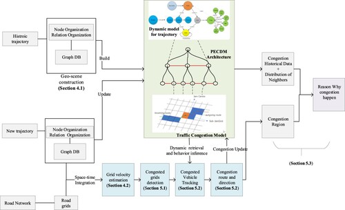
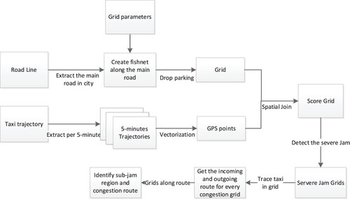
From the above work, it is clear that taxi trajectories contain many vehicle states that can reflect fine-grained traffic conditions when the sampling rate is sufficient. Therefore, fast organization and inference of immediate traffic states from spatio-temporal trajectories can aid congestion detection. To achieve this, it is necessary to establish a dynamic representation model of the spatio-temporal trajectories in massive volumes to support data organization and inference. This problem is tackled in this study. The overall approach of this paper is illustrated in Figure 1.

Figure 1. The flow of the work.

3. Model overview

To construct EPCDM for urban traffic congestion, this paper begins by discussing the six elements of geographic scene models (time, space, attribute, semantic, event, process) as they apply to urban traffic. A congestion event is usually composed of multiple slow or stalled vehicle travel processes. Vehicle travel processes consist of temporal vehicle states. The attributes of the vehicle states include speed, passengers, location (GPS point), direction and passenger status (empty or occupied).

Assuming that a taxi GPS point is generated every t seconds, the taxi dynamics process, denoted Process-t, consists of taxi states with a temporal sequence. The taxi process Process-t consists of a series of states S_t, which can be expressed as $\mathrm{P}\mathrm{r}\mathrm{o}\mathrm{c}\mathrm{e}\mathrm{s}\mathrm{s}-t=\{S_1,S_2,\dots ,S_t,\dots ,S_n\}$Concerning passengers in taxis, the driving process of a taxi can be divided into three sub-processes: passenger-carrying, empty (taxi without passengers looking for a passenger), and busy (i.e. doing something other than carrying passengers or waiting for passengers). The sub-processes do not overlap each other in time. From the perspective of congestion, driving can also be divided into a congestion sub-process Process_C and a normal driving sub-process Process_N. However, some sub-processes such as temporary parking, refueling/recharging, waiting for passengers, and driver breaks need to be distinguished from congestion.

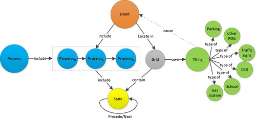
As to traffic congestion events, the congestion region aggregates one or more taxi slow driving sub-processes. For calculation purposes, the space is partitioned in the form of a grid. Within a grid cell, the metric attributes of the traffic flow are homogenized for speed assessment. The exploration of vehicle congestion within the study area is linked to the traffic flow along the road direction grid. An event contains multiple taxi congestion sub-processes; Taxi sub-processes consist of several continuously distributed states; A grid cell contains multiple states; Traffic congestion events are continuously located at grid cells, as Figure 2 shows. The ‘things’ in the urban traffic scene refer to gas stations, parking lots, schools, traffic signs, hospitals, shopping malls, restaurants, residential buildings, and others; most of them are classed as POIs. The POI distribution of grid cells often helps explain why congestion events happen. The interaction among those objects that portray the taxi dynamic process within the congestion model is shown in Figure 2.

Figure 2. Relationship diagram of spatio-temporal dynamics in congestion.

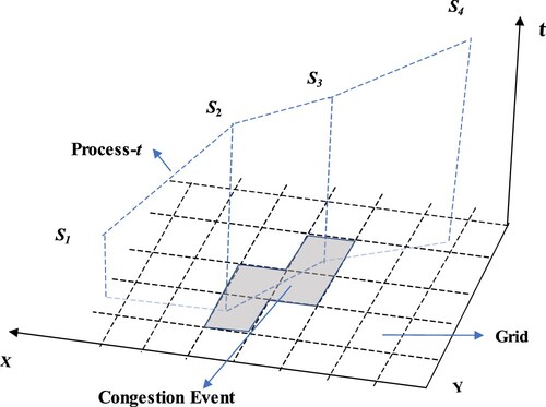
In the case of time, the taxi movement process is a spatial curve and consists of a series of spatio-temporal state points $S\left(x,y,t\right)$. A traffic congestion event is visualized as a composition of road segments corresponding to slow-moving vehicles, or congestion events that are composed of one or more neighboring grid cells distributed along the road. A schematic diagram of the taxi space–time object is shown in Figure 3.

Figure 3. State-process-event spatio-temporal diagram of taxis.

Traffic congestion has a congestion center in space, and sub-congestion areas are found along both directions of the road from the congestion center. This is illustrated in Figure 4, in which the orange grid cell is the central congestion area (consisting of one or multiple adjacent grid cells), and the blue grid cells are the sub-congestion area. According to the direction of traffic flow, road congestion can be divided into incoming congestion routes and outgoing congestion routes.

Figure 4. Diagram of a traffic jam geo-event.

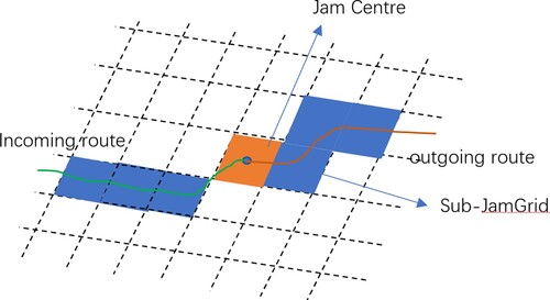
The two congestion route directions are relative to the direction of traffic flow. Since many roads have lanes in two directions, for a congestion grid, when the road is congested in both directions at the same time, based on the vehicle trajectory, the congestion grid cell has incoming and outgoing routes at the same time.

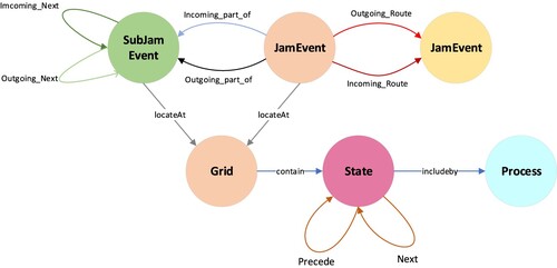
The translation of the traffic congestion geo-event structure into logical model results in the event detail model shown in Figure 5. As Figure 5 shows, the congestion center (JamEvent) links to each sub-congestion (SubJamEvent) grid, and each congestion event has incoming routes and outgoing routes. Both of them are located at Grids. Grid includes taxi states (GPS point); Process also includes states.

Figure 5. The structure of the traffic jam geo-event model.

Some of the taxi behaviors that can be identified from the trajectories in this model include dropping off and picking up passengers, driving with passengers, driving without passengers, changing shifts, stopping temporarily (for pick up/ drop off passengers), and entering and exiting car parks. Spatio-temporal characteristics of a congestion event refer to the start and end time and the grid cells where it takes place, while semantic information focuses on causes and effects of congestion, speed of traffic, and other properties such as scale and decay time. The average speed in the grid is an important parameter for detecting traffic jams. The scene objects (things, process, events and state) in the taxi scene are depicted in part I of Appendix 1.

4. Model implementation

The organization of dynamic data on traffic congestion usually involves a very large number of nodes and relationships. This section outlines the construction method of the dynamic model and the calculation of the average taxi velocity for each grid cell.

4.1. EPCDM construction in Neo4j

Following the storage strategy of previous studies (He et al. 2021), this study organizes and stores the data in a dynamic model structured according to the three major relationships – hierarchy, development, and inclusion – in Neo4j. According to Figures 1 and 4, those relationships are defined as follows:

• Development relationship: ‘Next/Precede’ between states, ‘Next/Precede’ between processes.

• Hierarchy/Inclusion relationship: the event contains sub-events, the event is located at grid cells, and the relationship between event and JamRoute.

• Mutual relationship: the grid includes states, the grid cell contains POIs, and the things result in event.

The scene relationships in taxi geo-scene are depicted in Part II of Appendix 1. The historical taxi trajectory data are partitioned into different comma-separated value file sequences with an interval of five minutes to construct the dynamic model. The model data are also updated every five minutes. This paper uses two algorithms to construct the model, as follows.

In Algorithm 1, first, the process and state nodes in the model are constructed. Then, the basic relationships are constructed: the containment relationships between processes and states, the temporal order (‘Next/Precede’) between the states, and the relationships between the states and grid cells.

Algorithm 2 is used to construct the relationships between events, grids, and congestion routes. First, according to the ‘included by’ relationship between the grid of the congestion center, filtered by the spatial join operation result, and the taxi state, the set of taxis in the congestion grid cell is obtained. Second, the travel trajectory of each taxi in the congestion area is used to identify the center-congestion and sub-congestion range. Third, the incoming and outgoing congested routes are found along the taxi trajectory. The detailed algorithms are depicted in Part III and IV of Appendix 1. Using Algorithms 1 and 2, an EPCDM for urban traffic is built. The relationship between POI and grid is easily constructed based on the topological inclusion.

4.2. Velocity evaluation for grid cells

To model vehicle movement across grid cells, it is necessary to calculate and characterize the flow velocity. A common method is to use a rule to describe the traffic congestion according to the interval average speed of urban trunk roads. A rule from the Chinese Ministry of Public Security in 2002 is shown in Table 1.

Table 1. A rule defining traffic congestion levels.

Level	Average speed(km/h)	Speed(m/s)
Smooth	>30	>8.33
Light congestion	[20,30)	5.56–8.33
Congestion	[10,20)	2.78–5.56
Severe congestion	<10	<2.78

Since main roads in cities are usually straight, most of them are less than the diagonal length of the grid. And if there are no GPS points in the grid cell, the speed of that grid cannot be identified from taxi GPS points.

When there is only one GPS data point, the vehicle speed must be greater than the speed of a vehicle that would record two points extremely distributed along the diagonal line, which corresponds to a traffic smooth state. Therefore, counting the number of GPS points in the grid in 5 min can be used to detect the speed of the traffic in the grid. The structure of the road is shown in Figure 6.

Figure 6. The structure of the road and grid.

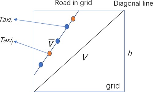
Assuming that h is grid length, k is the time interval between 2 GPS points (sampling rate), c is the number of points that exist in a grid for a taxi in the period T, the average speed is V of the taxi along the grid diagonal road is (1) $V=\sqrt{2}h/\left[k\left(c-1\right)\right].$(1) Assuming a common traffic light waiting time of 60 s, if the traffic flows smoothly, $\left[60/k\right]-1$ is the count of taxi GPS points where the taxi waiting time for traffic lights, where [] denotes the integer part. The number of points c present in the grid in 5 min must be greater than $\left[60/k\right]-1$ to filters out the effect of the traffic signal: (2) $\mathrm{c}>\left[{\displaystyle \frac{60}{k}}\right]-1.$(2) In the congestion detection process, most of the roads are shorter than the diagonal of the grid, therefore a congested grid can be identified by comparing $V$ with the grid average speed $\overline{V}$, with $V>\overline{V}$ indicating a congested grid.

Let the number of taxis in the grid be denoted by ‘count’. The number of GPS data points in the grid for any taxi i is C_i, by statistic the sum of all the taxi in grid in 5 min, because the road is shorter than diagonal line, the average speed in the grid $\overline{V}$ is (3) $\overline{V}<={\displaystyle \frac{{\sum }_{i=1}^{count}{\displaystyle \frac{\sqrt{2}h}{k{C}_i}}}{count}.}$(3) For traffic jam level S, the maximum speed in the grid is V_S, and the count of the points in the grid which meet the definition of this level of congestion is found by substituting C_S for $C$ in Equation (1), resulting in (4) $\{\begin{array}{c}{V}_S=\\ \sqrt{2}{\displaystyle \frac{n}{\left[k\left(C_S-1\right)\right]}}\\ C_S=\\ \left[1+{\displaystyle \frac{\sqrt{2}h}{\mathrm{k}{v}_S}}\right].\end{array},$(4) The condition for the detection of a congestion event, R, is (5) $R=\{\begin{array}{c}\mathrm{t}\mathrm{r}\mathrm{u}\mathrm{e}\\ \begin{array}{c}\overline{V}<V_s\\ \mathrm{a}\mathrm{n}\mathrm{d}\\ C_i>=min(Cs,\left[{\displaystyle \frac{60}{k}}\right]-1)\end{array}\\ \mathrm{f}\mathrm{a}\mathrm{l}\mathrm{s}\mathrm{e}\\ \mathrm{o}\mathrm{t}\mathrm{h}\mathrm{e}\mathrm{r}\mathrm{w}\mathrm{i}\mathrm{s}\mathrm{e}\end{array}.$(5) To detect the average speed along the road, the size of the grid needs to be suitable. Many studies have used a grid with a width greater than 500 m, which means that they could only identify the traffic flow in an urban grid and could not identify the speed of vehicles on the roads.

Suppose the sampling rate k is 10 s per point and the diagonal of the grid is 250 m, then the width is 180 m. Then, the threshold values of V_s and C_S are shown in Table 2. This methodology achieves the evaluation of the average velocity of the grid cell every 5 min in the model, and the calculation results are key to the model implementation and can be an indicator of traffic congestion.

Table 2. Detection parameters for different congestion levels.

Level	speed(km/h)	Speed(m/s)	Cs	Vs
Smooth	>30	>8.33	–	–
Light	[20,30)	5.56–8.33	4	8.33
Congestion	[10,20)	2.78–5.56	6	5.56
Severe	<10	<2.78	10	2.78
Severe +	<5	1.38	19	1.38

5. Congestion detection

In this section, the procedure for detecting congestion is outlined.

5.1. Detection of congestion grid cells

To achieve sufficient temporal resolution while limiting computational demands, the trajectory data are split into multiple trajectory files according to the 5-minute interval duration.

To detect congestion, first the Spatial Join operation in ArcGIS is performed between the grid layer and the 5-minute spatial point layer of the taxi data, and the average speed and the maximum number of GPS points in the grid cell in five minutes are calculated according to the relationship between the grid objects and states in the model. Next, the corresponding thresholds V_k (the maximum average speed) and C_s (the minimum count of GPS points), according to the congestion level, are set to detect the congestion condition in the grid cells. Taking the detection of a severely congested area as an example, first, the distribution of severely congested grid cells is found. Then the congested routes are identified based on the trajectory of vehicles in the congested area. Finally, sub-congestion parameters along the road are set to extract the sub-congestion grid and form a two-level congested road structure. A detailed flow diagram of the procedure is shown in Figure 7.

Figure 7. A flow diagram of the algorithm for detecting traffic jams.

5.2. Congestion direction detection

Most roads in the city are two-way roads, and both two-sided congestion and one-sided congestion on the roads are common phenomena. With the fast retrieval and data organization capabilities provided by the constructed model, the proposed method can also identify the direction of congestion and the level of congestion. Using the Neo4j neosemantics toolkit and logical relationships between events, processes, and states, the vehicle routes in congested areas can be reasoned about and tracked, which greatly enhances the ability to find congestion details, such as tracking the vehicles in the congested area and identifying the route of the congestion.

Thus, the method in this article tracks the vehicles’ incoming and outgoing routes and also obtains the sequence of grid cells of the incoming and outgoing routes. If these grids are continuously distributed and adjacent to the congestion center grid cells, and their average speed is less than the core congestion parameters, they are incoming and outgoing sub-congestion areas.

Based on the parameters of taxi ID (taxiid) and the time of state (Cur_Time) in the congestion grid, the Cypher query CQ1 finds the travel trajectory sequence from the passengers’ pick-up points to the current congestion area or in a given period, and the query CQ2 finds the trajectory of the taxi from the congested area to passengers’ drop-off points or in a given period. The full details of these queries are as follows.

CQ1:Match (cat:Process{taxiid:$taxiid} CALL n10s.inference.nodesInCategory (cat,{inCatRel:‘IncludeBy’, subCatRel:‘Next’}) yield node match (node)-[]->(ss:State {Passenger:0 }) where node.Passenger=1 and toInteger(node.Xh)<= toInteger($cur_Time) with node match (node)-[r:Contain]- (g:Grid) with node,g ORDER BY node.Xh DESC limit 1 return node.Name as Name,g.GridId as Grid,node.X as X,node.Y as Y,node.Xh as Xh,g.MaxPts as MaxPts,g.AvgSpeed as AvgSpeed;

CQ2: Match (cat:Process{taxiid:$taxiid}) CALL n10s.inference.nodesInCategory(cat,{inCatRel:‘IncludeBy’, subCatRel:‘Next’}) yield node match (node)-[]->(ss:State {Passenger:0 }) where node.Passenger=1 and toInteger(node.Xh)> toInteger($cur_Time) with node match (node)-[r:Contain]- (g:Grid) with node,g ORDER BY node.Xh DESC limit 1 return node.Name as Name,g.GridId as Grid,node.X as X,node.Y as Y,node.Xh as Xh,g.MaxPts as MaxPts,g.AvgSpeed as AvgSpeed;

When there are slow-moving vehicles in both directions in the congested area, the road is congested on both sides. If the speed of vehicles in one direction is normal and the speed of vehicles in the other direction is slow, the road is congested on one side. If slow vehicles on one side are identified and vehicles in the other direction are not recorded, the congestion area can only detect congestion on one side and the other side is unknown. Since the length of the incoming or outgoing route is known within the congestion area and the stagnation points of that vehicle in the route can be counted, the calculated average speed is bound to be a more accurate estimate than the first evaluation. And this new speed can be used to improve the average speed of the corresponding time in the congestion area.

Along the incoming and outgoing route, severe congestion event grid cells, sub-congestion grid cells, and congestion routes are obtained. According to the structure of the traffic jam geo-event model in Figure 5, hierarchical congestion event results can be constructed. The model has a powerful retrieval capability, avoiding repeated spatial analysis, which would be computationally expensive. The query CQ3, which quickly finds bidirectional congestion in the grid cell of gridid is as follows.

CQ3:MATCH(je:JamEvent{grid:$gridid})-[]-(je2:SubJamEvent) where (je)-[:outgoing_part_of]-(je2) and (je)-[:incoming_part_of]-(je2) with je,je2 match(je2)-[:locateAt]-(g:Grid) with g,je,je2 match (je)-[]-(jr:JamRoute) return je,je2,jr,g;

5.3. Causes of congestion events

Understanding the correlation between the grid and the surrounding POIs helps to extract the distribution of environmental factors that may be related to congestion events. In general, except for traffic accidents, each type of congestion is associated with a statistical model of spatial and temporal vehicle behavior. Such statistical characteristics are in turn closely related to the POIs surrounding the congestion. Modeling the congestion behavior and the distribution of surrounding POIs can reveal the causes of congestion.

Using the dynamic model to extract individual vehicle behavior, it is possible to efficiently obtain a statistical model of vehicle behaviors such as the distribution of passengers’ pick-up and drop-off points, the distribution of start and end points of taxis passing by a given region, the arrival times of passengers in a given region, or the distribution of empty taxis. Some taxi behaviors and traffic flows are significantly correlated with the distribution of surrounding POIs, such as schools and zebra crossings, intersections and traffic lights, residential areas, CBDs, tunnels and bridges, and different types of restaurants.

Employing data mining to extract patterns in the distribution of taxi behavior related to the distribution of environmental factors in terms of data mining is also a worthwhile area of research. Here, a thought is proposed to use the taxi behavior model to obtain the cause of congestion by identifying the statistical characteristics associated with the POI distribution around a congestion event is explained by example in Section 6.

6. Case study and analysis

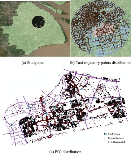
To validate and demonstrate the effectiveness of the model, this paper used taxi trajectory data from Shanghai from 17:00–19:30 on April 11, 2015. These data were used to detect traffic congestion events in Pudong along the Huangpu River and to identify the causes of these events. The experimental data set is the Shanghai taxi trajectory data (CSV format) from April 1 to April 30, 2015, with over 10,000 taxis and a sampling rate of one point every 10 s, so that about 200,000 floating-point coordinates were generated every 5 min. As shown in Figure 8(a), the taxi trajectory data within a 10 km radius of the Mercedes-Benz Arena, located in Shanghai’s CBD, were selected for modeling. Figure 8(b) shows the 10 km range: brown points represent taxi trajectory points (from 17:10–17:15) and the traffic event detection area is represented by a red polygon. Figure 8(c) shows the POI distribution and subway stations. The width of the grid along the road is 180 m. By dividing the trajectory data into 5-minute intervals, the sample data were divided into a total of 30 sets of trajectory data. Following the method outlined in section 4, the traffic flow was segmented by counting the average speed within a grid cell and the number of maximum taxi detection points in a 5-minute range.

Figure 8. Study area and taxi trajectory data distribution.

6.1. Model construction steps and congestion detection

The process of model construction can be divided into two steps: (a) establishing a spatio-temporal ‘event-process-state’ dynamic model for floating taxis and (b) detecting traffic congestion using the model. As discussed in section 4.1, Algorithms 1 and 2 implement the construction of the objects and relations involved in the processes and states of the model. The relationships between the grid and the taxi state points are built using spatial statistics. Due to the large number of data nodes and relationships, when building the Neo4j database, the historical data were imported offline using batch-import, and the updated data were imported online using the function ‘Load CSV’. The structure of the nodes exported by Algorithms 1 and 2 was organized as shown in Table 3. The structure of the exported relationships is shown in Table 4. The construction plan of a complete real-time traffic congestion detection system is shown in Part V of Appendix 1. And data pre-processing (see Part VI of Appendix 1) was necessary before model construction.

Table 3. The structure of a state node.

:LABEL	GridId:ID	AvgSpeed	MaxPts	Time	X	Y	Count	Staycount
State	S42144366

Table 4. The structure of a relationship.

:START_ID	:END_ID	:TYPE
Grid0411171000001	S42144366	contain

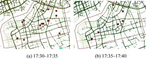
After constructing the taxi dynamic model and setting the speed and point count detection thresholds, congestion locations were identified from the grid cells which contained average speed and detection points within 5 min that were above the thresholds. For example, for the ‘severely congested’ parameters, the congestion status of each grid cell from 17:30–17:40 is shown in Figure 9.

Figure 9. Distribution of severely congested grids(red rectangles) within 17:30–17:40 on April 11.

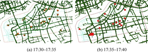
Setting the parameter threshold to the general congestion level, the congestion status in each grid cell from 17:30–17:40 is shown in Figure 10.

Figure 10. Distribution of generally congested grid cells from 17:30–17:40.

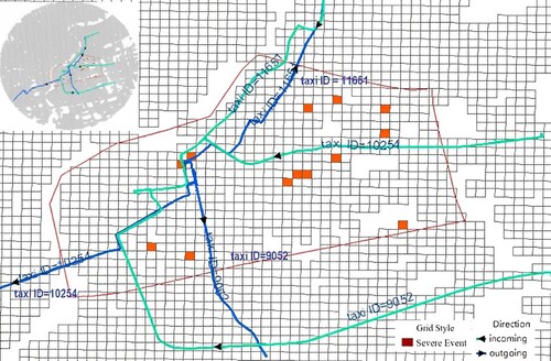
The center congestion (grid cell id 2976), shown in Figure 11, was taken as an example to deduce three trajectories through the congestion center, using the queries CQ1 and CQ2. These trajectories have incoming and outgoing parts respectively.

Figure 11. Three trajectories through the congestion center.

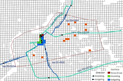
Along the trajectory route, by judging whether the speeds of the adjacent grid cells converge to the sub-congestion parameters, the incoming and outgoing grid cells are shown in Figure 12, in which some grid cells with dual directions (outgoing and incoming) can be seen. It can be seen that the grid within the dashed line displays congestion in both directions, based on the number of GPS points left incoming at 1.48 m/s and outgoing at 2.3 m/s, which both fall in the extremely congested category.

Figure 12. Sub-congestion grid cells of the severe congestion grid.

6.2. Organization and visualization of hierarchical congestion event

Based on the model of traffic congestion designed in this paper, the detection results were automatically stored in the graph database. Figure 13 shows how the congestion results of grid 2581 (the red node from Figure 13) from 17:35–17:40 are organized. There are three taxis with IDs 1531, 6423, and 5922 crossing the congestion grid cell. Along the way, the grid cells which are connected to the congestion grid cell are the sub-congestion grid cells (green nodes); they are connected to other grid cells by the congestion routes (orange nodes) of the congestion event. From the structure, the congestion route of every taxi in each congestion grid can be traced. Setting gridid equal to 2581, the bidirectional congestion structure of the traffic jam event in grid 2581 can quickly be found as shown in Figure 14.

Figure 13. Graph structure of the traffic jam event in Grid 2581.

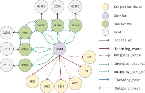
Figure 14. Detection of bidirectional traffic jam events.

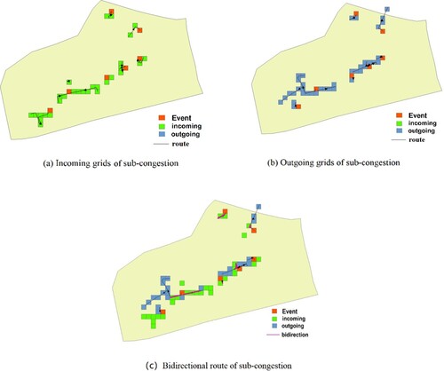
Figure 14(a) shows the tracked incoming paths, and Figure 14(b) shows the tracked outgoing paths. The red grid cells are the congestion core area. The red route in Figure 14(c) shows the two-way congestion routes that were detected. It can be observed that the red route is the corresponding grid cell with traffic flowing in opposite directions at the same time.

6.3. Analysis of the causes of congestion

Common causes of traffic congestion include the morning peak, the evening peak, major events within the detection area, road maintenance, traffic accidents, and adverse weather conditions. With the advantages of dynamic models in extracting individual vehicle behaviors, corresponding statistical models for each different kind of congestion can identify the causes of congestion.

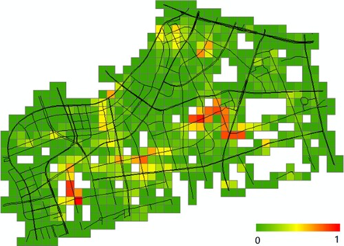
Suppose there exist m sets of 5-minute trajectory data layers, Cgrid_i denotes whether the ith trajectory layer is a congested area (taking the value of 1 for congested and 0 for non-congested), then the average parameter η is (5) $\eta ={\displaystyle \frac{{\sum }_{\mathrm{i}=0}^{m-1}C\mathrm{g}\mathrm{r}\mathrm{i}{\mathrm{d}}_i}{m}}$(5) Using Equation (5), the congestion indicator was calculated for 30 sets of trajectory layer data, and the indicator values were in the range of [0, 30]. The resulting distribution is shown in Figure 15, where the redder the color, the more serious the congestion, with the green areas representing smooth traffic flow. There are four more obvious congestion areas in Figure 15, three in the center of the study area and one in its upper part.

Figure 15. Congestion indicator distribution from 17:00–19:30 on April 11.

An interpretation of the causes of congestion can be provided by overlaying taxi trajectory layers, points of interest, taxi drop-off areas, and local knowledge. By observing changes in the passenger states of the taxis, the pick-up point or drop-off point can be found. The pick-up point extraction sets the passenger pre-state to 0 and the post-state to 1; the reverse is true for the drop-off point. The query CQ4 for the pick-up points is as follows.

Match ((node)-[]->(ss:State {Passenger:0 }) where node.Passenger=1 and toInteger(node.Xh)<= toInteger($End_Time) and toInteger(node.Xh)>= toInteger($Start_Time) with node match (node)-[r:Contain]- (g:Grid) with node,g ORDER BY node.Xh DESC limit 1 return node.Name as Name,g.GridId as Grid,node.X as X,node.Y as Y;

Using CQ4, the coordinates of the pick-up and drop-off points, and the corresponding grid cells at the specified timespan (Start_Time to End_Time), were obtained. After point density analysis, and amount statistics by grid cell, the different areas of pick-up and drop-off behaviors were obtained. POI numbers and percentages were counted in those hotpot grid cell areas to like the local knowledge situation (shown in Figure 16).

Figure 16. Hotspot distribution of drop-off taxis from 17:00–22:00 on April 11 and April 25.

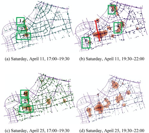
Comparing the congestion zone map with the distribution of restaurant and residential area POIs (as in Figure 16(b)) shows that vehicle congestion is closely related to the POI distribution. In congestion areas 4, 5, and 6, it can be seen that the congestion factor is high in residential areas. In congestion areas 1, 2, and 3 (as in Figure 16(a)), there is a high density of restaurants, so the congestion events were likely related to high numbers of people eating out on weekends from 17:00–19:30.

Using the method in this paper, the drop-off areas between 17:00–19:30 on April 11 were extracted. From 17:00–19:30 on a Saturday, vehicle drop-offs were clustered on Shangnan road (Figure 16(b) red line), which is highly relevant to the reason for drop-offs for meals. By the 19:30–22:00 period, the drop-off areas were dispersed, but there was still a cluster on the original road. As Figure 16(b) shows, area 1 still showed aggregation, but the number of vehicles in the area decreased from 300 to 30 compared to at 17:00–19:30. In area 3, the distribution was steady from 19:30–22:00, although this congestion was also related to restaurants – the horizontal street in area 3 is the night market, where people often buy snacks in the evening. For areas 4, 5, and 6 at 19:30–22:00, on April 11, residents who went out for fun or shopping during the day were returning home.

The distribution of the drop-off areas on the other weekend (April 25) is shown in Figure 16(c)(d). Similar to April 11 in general, there is still a strong influence from restaurants and residential areas. On April 25 from 17:00–19:30, drop-off areas were more concentrated in the restaurant street but were lower than on April 11 in terms of both volume and density.

A closer look at area 1 shows that the number of vehicles gathered within Area 1 from 17:00–19:30 was about 50, and from 19:30–22:00 there were less than 20 vehicles on April 25. Compared to the same period on April 11, the number of vehicles dropped off during 17:00–19:30 on April 25, being almost 300 vehicles less than the number during the same period on April 11, but there was little difference from 19:30–22:00.

Dining area 2 also shows a significant change, with a total of 314 drop-offs from 17:00–19:30 on April 11, and only 51 drop-offs during the same period on April 25; after 19:30, the number of drop-offs does not change much.

In area 3, from 17:00–19:30, on April 11 there were 306 drop-offs, while on April 25 there were 95. There was a significant decrease in the number of drop-offs in the food street, while there was no significant change in the residential area.

The detailed changes in drop-off taxi volumes for the congestion described above are shown in Table 5. By exploring the events that occurred between 17:00 and 22:00 on both days, it is found that the Mercedes-Benz stadium is two hundred meters away from the location of area 1, and on April 11, more than 12,000 people attended a concert in that stadium by the musician JJ Lin. Before the concert started, the fans had enough time to be the first to arrive at the food street to eat their evening meal, which led to a larger than usual drop-off area at the food street, which also led to a congestion problem in areas 1, 2, and 3 before the concert on April 11. On April 25, there was no significant event at the Mercedes-Benz Stadium from 17:00–19:30, as Figure 17 shows. The concerts were the main cause of congestion around the food court and the Mercedes-Benz Stadium.

Figure 17. Traffic congestion distribution from 17:00–19:30 on April 25.

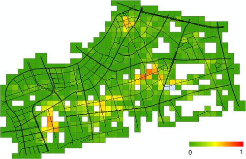
Table 5. Drop-off count of taxis in different areas in Figure 16(b).

	Area 1	Area 2	Area 3
April 11 17:00–19:30	353	314	306
April 11 19:30–22:00	27	14	56
April 25 17:00–19:30	50	51	95
April 25 19:30–22:00	18	17	65

6.4. Accuracy and efficiency

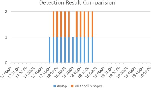
The data in this paper are historical trajectories in 2015, which cannot be compared with the actual traffic conditions at that time to evaluate the accuracy. Therefore, we re-adopt the trajectory data on December 7, 2022 to evaluate the accuracy, and the comparison experiment is conducted with real-time congestion data of AMap. Crawling AMap congestion data on South Xizang Road Tunnel exit (Pudong part) from 5 pm to 8 pm using python (https://restapi.amap.com/v3/traffic/status/road?name=load name& adcode = city-code & key = yourKey &extensions = all). The time resolution of AMap road congestion data and the method in this paper is the same as 5 min, the road congestion status is marked as 1, and the non-congestion is marked as 0. The result is shown in Figure 18, the South Xizang Road Tunnel exit (Pudong part) has congestion by Off-duty evening peak during 17:50–18:45. AMap uses a combination of data from crowdsourced vehicles running on the road and the traffic facilities of the traffic authority for congestion detection, which is recognized as the accurate and one of the most commonly used method of congestion detection and navigation in China. Since the vehicle data of the method in this paper is not as perfect as that of AMap, the congestion in this paper cannot be detected when there is no cab on the road. In our test results, Amap's method found 12 consecutive congestions in the South Xizang Road tunnel exit (Pudong part), and the method in this paper detected 10 consecutive congestions. The accuracy calculation formula is listed below: (5) $\mathrm{R}={\displaystyle \frac{\mathrm{C}\mathrm{P}}{CAMAP}\ast 100\text{\%}}$(5) CP refers to the congestion scores in our method, and CAMAP is the score of AMap. Therefore, the accuracy of our paper is 83.3%. Our approach is highly dependent on the number of vehicles.

Figure 18. Detection accuracy comparison between AMap and method in the paper.

Thus, the model in this paper has an appreciable accuracy in experiments. And all the congestion points and congestion directions detected by the method in this paper are correct. This is because each congestion grid is obtained by the secondary identification of taxis according to the congestion level. In terms of efficiency, the retrieval time consumed for taxi behavior in this paper is several milliseconds, and the retrieval of the drop-off and pick-up points of all Shanghai cabs within 3 h can also be achieved within 1 s, which has a favorable experience for users.

7. Summary and conclusions

This paper established a dynamic model of urban traffic congestion based on events and processes. The abstraction of traffic into events, processes, and states represents taxis as states and the taxi driving process as a state sequence, and identifies areas of slow vehicle speed as congestion. According to the development process of traffic congestion, the congestion outgoing and incoming area, and the traffic congestion route, a congestion event is organized as a logical structure of traffic congestion. This representation allows the storage of historical traffic congestion information.

The dynamic model is implemented in the form of a graph database representing the development, inclusion, and nesting relationships among states, processes, events, and grid cells. The average speed of the road is calculated from the average speed of the vehicles in the 5-minute grid, and the maximum speed of the road is evaluated by counting the number of GPS points sampled on the grid. The core congestion area is identified based on a speed criterion, and the incoming route grid cells and outgoing route grid cells are searched by identifying the trajectories of vehicles within the congestion area and the speed of the grid cells respectively; this approach finally leads to the extraction of the congestion route.

The method in this paper overcomes the disadvantages due to the low resolution of traditional models, while avoiding the limited detection range and high expense of video monitoring methods. In addition, it can identify two-way congestion, and the organized structure of the event history data facilitates the investigation of traffic congestion and the retrieval of detailed historical congestion information. The representation of the processes and events as well as related POIs in the graph database also provides new methods for analyzing the causes of congestion.

This paper not only provides a method for constructing the model but also provides a data update mechanism for adding new data. The constructed methods have the potential to detect the current state of traffic congestion in a specified area, with data added to the graph database in real time.

Nevertheless, the approach in paper has some limitations. First, the grid division strategy uses straightforward full network equalization, which inevitably results in varying road lengths within each grid. The detection method assumes that the maximum length within the grid cells is the diagonal length, and when the road length is greater than the diagonal, the average speed of the grid may be underestimated (this situation is rare). However, when the road is smaller than the diagonal (a common situation), the average speed of the grid is overestimated. In this case, the proposed method detects a speed in the congestion zone greater than or equal to the true speed, thus possibly ignoring some grid cells that may belong to the congestion zone. Future work will deal with proposing a spatial division method aiming at the uniform division of roads, which should mitigate this problem.

Second, the grid speed derivation method, based on taxi GPS points, can be inaccurate in areas with low taxi density. The more taxis there are, the more sensitive and accurate the method is for the detection of traffic congestion and congested routes. In this paper, the taxi GPS sampling rate is once every 10 s, and the sample thinning reduces the computational complexity and makes the algorithm run faster, but it will also have some influence on the accuracy.

Third, the method in paper has limited effectiveness in monitoring congestion in areas where elevated lanes overlap with roadway lanes, and improvement by combining elevation of GPS point will be the next research task.

The method in this paper is implemented using EPCDM, which is based on the relationship between events, processes, states, and things. This paper has demonstrated its advantages in spatio-temporal retrieval and spatio-temporal reasoning. But besides the identification of traffic congestion situations, the method should also be capable of predicting traffic congestion. Further work could combine the method in this paper detects with machine learning methods to develop a highly capable traffic prediction model.

Data and codes availability statement

The traffic congestion database file that support this study can be obtained from https://github.com/Yufeng05He/TrafficCongestionModel/releases/download/V1.0.0/neo4j.7z (last accesses 05 October 2022).

The CSV files which is used to database construction was provided in the link: https://github.com/Yufeng05He/TrafficCongestionModel/releases/tag/V1.0.0/CSV.files.zip (last accesses 05 October 2022).

Disclosure statement

No potential conflict of interest was reported by the author(s).

Additional information

Funding

This work was supported by National Natural Science Foundation of China [grant number 42071364 and 41631175].

References

- Azimi, M., and Y. Zhang. 2010. “Categorizing Freeway Flow Conditions by Using Clustering Methods.” Transportation Research Record: Journal of the Transportation Research Board 2173 (1): 105–114. doi:10.3141/2173-13
- Bittner, T., M. Donnelly, and B. Smith. 2004. “Endurants and Perdurants in Directly Depicting Ontologies.” AI Communications 17 (4): 247–258. doi:10.5555/1080472.1080480.
- Chen, M., C. Yang, T. Hou, G. Lü, Y. Wen, and S. Yue. 2018. “Developing a Data Model for Understanding Geographical Analysis Models with Consideration of Their Evolution and Application Processes.” Transactions in GIS 22 (6): 1498–1521. doi:10.1111/tgis.12484
- Cui, J., F. Liu, J. Hu, D. Janssens, G. Wets, and M. Cools. 2016. “Identifying Mismatch Between Urban Travel Demand and Transport Network Services Using GPS Data: A Case Study in the Fast Growing Chinese City of Harbin.” Neurocomputing 181: 4–18. doi:10.1016/j.neucom.2015.08.100
- D’Andrea, E., and F. Marcelloni. 2017. “Detection of Traffic Congestion and Incidents from GPS Trace Analysis.” Expert Systems with Applications 73: 43–56. doi:10.1016/j.eswa.2016.12.018
- Devaraju, A., W. Kuhn, and C. S. Renschler. 2015. “A Formal Model to Infer Geographic Events from Sensor Observations.” International Journal of Geographical Information Science 29 (1): 1–27. doi:10.1080/13658816.2014.933480
- Galton, A. 2012. “The Ontology of States, Processes, and Events.” Mathematics of Control Signals & Systems 22 (1): 1–22.
- Goodchild, M. F., M. J. Egenhofer, K. K. Kemp, D. M. Mark, and E. Sheppard. 1999. “Introduction to the Varenius Project.” International Journal of Geographical Information Science 13 (8): 731–745. doi:10.1080/136588199240996
- Grenon, P., and B. Smith. 2004. “SNAP and SPAN: Towards Dynamic Spatial Ontology.” Spatial Cognition & Computation 4 (1): 69–104. doi:10.1207/s15427633scc0401_5
- He, Y., B. Hofer, Y. Sheng, and Y. Huang. 2021. “Dynamic Representations of Spatial Events – The Example of a Typhoon.” AGILE GIScience Ser 2: 30. doi:10.5194/agile-giss-2-30-2021.
- He, Y., Y. Sheng, B. Hofer, Y. Huang, and J. Qin. 2022. “Processes and Events in the Centre: A Dynamic Data Model for Representing Spatial Change.” International Journal of Digital Earth 15 (1): 276–295. doi:10.1080/17538947.2021.2025275
- Huang, Y., M. Yuan, Y. Sheng, X. Min, and Y. Cao. 2019. “Using Geographic Ontologies and Geo-Characterization to Represent Geographic Scenarios.” ISPRS International Journal of Geo-Information 8 (12): 566. doi:10.3390/ijgi8120566
- Johansson, I. 2005. Qualities, Quantities, and the Endurant-Perdurant Distinction in Top-Level Ontologies. Kaiserslautern, Germany: Wissensmanagement.
- Kan, Z., L. Tang, M.-P. Kwan, C. Ren, D. Liu, and Q. Li. 2019. “Traffic Congestion Analysis at the Turn Level Using Taxis’ GPS Trajectory Data.” Computers, Environment and Urban Systems 74: 229–243. doi:10.1016/j.compenvurbsys.2018.11.007
- Langran, G., and N. R. Chrisman. 1992. “A Framework For Temporal Geographic Information.” Cartographica: The International Journal for Geographic Information and Geovisualization 25 (3): 1–14. doi:10.3138/K877-7273-2238-5Q6V
- Lin, H., M. Chen, G. Lu, Q. Zhu, J. Gong, X. You, Y. Wen, B. Xu, and M. Hu. 2013. “Virtual Geographic Environments (VGEs): A New Generation of Geographic Analysis Tool.” Earth-Science Reviews 126: 74–84. doi:10.1016/j.earscirev.2013.08.001
- Liu, C., K. Qin, and C. Kang. 2015. “Exploring Time-Dependent Traffic Congestion Patterns from Taxi Trajectory Data.” 2015 2nd IEEE international conference on spatial data mining and geographical knowledge services (ICSDM), IEEE.
- Lü, G., M. Batty, J. Strobl, H. Lin, A.-X. Zhu, and M. Chen. 2019. “Reflections and Speculations on the Progress in Geographic Information Systems (GIS): A Geographic Perspective.” International Journal of Geographical Information Science 33 (2): 346–367. doi:10.1080/13658816.2018.1533136
- Lu, G. N., M. Chen, L. W. Yuan, L. C. Zhou, Y. N. Wen, M. G. Wu, B. Hu, Z. Y. Yu, S. S. Yue, and Y. H. Sheng. 2018. “Geographic Scenario: A Possible Foundation for Further Development of Virtual Geographic Environments.” International Journal of Digital Earth 11 (4): 356–368. doi:10.1080/17538947.2017.1374477
- Salman, S., and S. Alaswad. 2018. “Alleviating Road Network Congestion: Traffic Pattern Optimization Using Markov Chain Traffic Assignment.” Computers & Operations Research 99: 191–205. doi:10.1016/j.cor.2018.06.015
- Wang, J., W. Deng, and Y. Guo. 2014. “New Bayesian Combination Method for Short-Term Traffic Flow Forecasting.” Transportation Research Part C: Emerging Technologies 43: 79–94. doi:10.1016/j.trc.2014.02.005
- Williams, N., S. Zander, and G. Armitage. 2006. “A Preliminary Performance Comparison of Five Machine Learning Algorithms for Practical IP Traffic Flow Classification.” ACM SIGCOMM Computer Communication Review 36 (5): 5–16. doi:10.1145/1163593.1163596
- Worboys, M. 2005. “Event-Oriented Approaches to Geographic Phenomena.” International Journal of Geographical Information Science 19 (1): 1–28. doi:10.1080/13658810412331280167
- Worboys, M., and K. Hornsby. 2004. “From Objects to Events: GEM, the Geospatial Event Model.” International conference on geographic information science, Springer.
- Wu, C., Q. Zhu, W. Xu, Y. Zhang, X. Xie, Y. Ding, F. He, and Y. Zhou. 2015. “A Real-Time geo-Processing Database Engine Linking Calculations and Storage for VGE.” Annals of GIS 21 (4): 265–274. doi:10.1080/19475683.2015.1057226
- Yu, B., H. Yin, and Z. Zhu. 2017. “Spatio-Temporal Graph Convolutional Networks: A Deep Learning Framework For Traffic Forecasting.” arXiv preprint arXiv:1709.04875.
- Yuan, M. 2001. “Representing Complex Geographic Phenomena in GIS.” Cartography and Geographic Information Science 28 (2): 83–96. doi:10.1559/152304001782173718
- Zhang, S., J. Tang, H. Wang, Y. Wang, and S. An. 2017. “Revealing Intra-Urban Travel Patterns and Service Ranges from Taxi Trajectories.” Journal of Transport Geography 61: 72–86. doi:10.1016/j.jtrangeo.2017.04.009