A knowledge-based approach for estimating the distribution of urban mixed land use

ABSTRACT

Estimating the proportion of land-use types in different regions is essential to promote the organization of a compact city and reduce energy consumption. However, existing research in this area has a few limitations: (1) lack of consideration of land-use distribution-related factors other than POIs; (2) inability to extract complex relations from heterogeneous information; and (3) overlooking the correlation between land-use types. To overcome these limitations, we propose a knowledge-based approach for estimating land-use distributions. We designed a knowledge graph to display POIs and other related heterogeneous data and then utilized a knowledge embedding model to directly obtain the region embedding vectors by learning the complex and implicit relations present in the knowledge graph. Region embedding vectors were mapped to land-use distributions using a label distribution learning method integrating the correlation between land-use types. To prove the reliability and validity of our approach, we conducted a case study in Jinhua, China. The results indicated that the proposed model outperformed other algorithms in all evaluation indices, thus illustrating the potential of this method to achieve higher accuracy land-use distribution estimates.

KEYWORDS:

• Knowledge graph
• land-use distribution
• region embedding
• label distribution learning
• label correlation

1. Introduction

In the information field, urban economic activities and human activities, constantly reshaping their spatial–temporal relationship and land-use distributions within cities (Andris 2016). In the twenty-first century, the formation of new industrial spaces and multi-center structures within cities began (Portnov and Schwart 2009). Thus, methods that enhance the vitality of people-centered cities are regarded as significant in this new era of urban development. Investigations into urban land-use distributions using urban computing methods (Zheng et al. 2014) are pivotal for understanding ‘human-land’ relationships, assisting the allocation of urban resources, and promoting urban sustainability.

In previous studies, uses of land in a single region were generally assumed to be homogeneous and were typically grouped into a single category (Niu et al. 2017; Wu et al. 2018; Zhou and Fan 2022). However, cities are usually composed of regions with various land-use types, such as for commercial, transportation, and water. Moreover, it is more realistic that land in a single region has multiple uses than a single use. Promoting diverse land-use types in a region can reduce commuting costs relatively, improve urban vitality, and make the city structure more compact (Burton, Jenks, and Williams 2003; Yue et al. 2017; Huang et al. 2022). This has been corroborated by previous studies estimating land-use distributions (i.e. the proportions of each land-use type) (Zhang et al. 2021; Huang et al. 2022). Zhang et al. (2021) utilized a random forest (RF) model, while Huang et al. (2022) adopted a multilayer perceptron (MLP) to assess the mixed land-use distributions, which both achieved satisfactory results in estimating land-use type proportions of various regions. Nevertheless, the aforementioned models assume that land-use categories are independent of each other; however, in reality, there are correlations between categories such as forest and greenland (Zhou, Xue, and Geng 2015; Ren et al. 2019).

Traditional methods are limited by the quality and quantity of samples; thus making it difficult to accurately characterize the relationship between regions and land-use types. Although remote sensing images have been widely used in land-use classification and urban functional area identification (Wang, Wu, and Wu 2012; Hong et al. 2021; Wang et al. 2022), the methods derived from pure remote sensing images can only reflect the natural characteristics of ground objects (Yao et al. 2017). In fact, the land-use distribution in a region is strongly correlated with the internal social and economic activities, which are difficult to determine from remote sensing images alone (Tu et al. 2017; Yao et al. 2017). The emergence of big urban data (e.g. social media data, human activity data, and point-of-interest (POI) data) provides a new perspective for exploring the urban land-use distribution (Yuan, Zheng, and Xie 2012; Han, Yu, and Long 2016, Li et al. 2021a, 2021b). Among them, POIs are open-source data that have been widely used for this topic due to their availability, fine granularity, and information richness (Gao, Krzysztof, and Helen 2017; Andrade, Alves, and Bento 2020; Zheng et al. 2020). To the best of our knowledge, the conventional POI-based approach involves capturing the regional spatial and semantic features from the POI data, translating those features into regional representation vectors, and subsequently inputting the regional representation vectors into downstream classification models. Thus, the primary challenge is to construct reasonable and complete regional representations of land-use distribution from POI data. Early studies often used manual engineering methods to construct features (Tian and Shen 2011; Jiang et al. 2015; Ma et al. 2022; Zhou and Fan 2022). However, such methods rely on the manual selection of quantitative indicators (e.g. frequency, density, and importance evaluation), and consider only surface features, which could lead to a loss of inner semantic relevance. To address the above research gap, representation learning (RL) methods have been used to automatically discover spatial and semantic features (Bengio, Courville, and Pascal 2013), with Word2vec being the most used RL model. Word2Vec is a typical natural language processing (NLP) model that expresses words as high-dimensional semantic vectors that can be understood by computers (Yao et al. 2017). Using a semantic model and embedded POI vectors with Word2Vec, Yao et al. (2017) and Yan et al. (2017) obtained a representative region distribution. Although the semantic method has advantages in capturing the semantic relationship between the POI categories, it has a limited capacity to capture the spatial features of POIs.

Moreover, although POIs are a competent proxy for sensing land-use distributions (Huang et al. 2022), multiple external factors (e.g. spatial proximity of regions and administrative divisions) affect urban functions. To account for this, Yan et al. (2017) proposed the Place2vec model which added distance to augmented spatial contexts to offset the shortage of characteristic spatial features by using only POI category semantics. Previous studies included certain external factors to enhance their model land-use classification accuracy. However, these models are usually only applicable for specific elements and are therefore unsuitable for the generalization to more complex and heterogeneous factors.

The concept of knowledge graphs (KG) was first proposed by Google to provide an effective way to structurally organize heterogeneous information. Due to their rich semantics, user-friendly structure, and high-quality information (Jiang et al. 2018), KGs can be used to compose semantic networks of entities with attributes and semantic relations to specific tasks such as question-answering systems (Xu et al. 2016) and search engines (Kasneci et al. 2008). However, as KGs contain many entities and semantic relations, extracting complex features and potential associations is key to enabling the further application of KGs to downstream learning tasks (Yang et al. 2022), such as information extraction (Hoffmann et al. 2011), text classification (Bayer, Kaufhold, and Reuter 2022), and spatio-temporal predictions (Zhu et al. 2022).

Considering the advantages of KGs in heterogeneous information expression, overcoming the shortcomings of single POI data use in feature representation and the limitation of conventional representation learning models in feature extraction, we propose an enhanced knowledge approach for evaluating urban land-use distribution. To our knowledge, this approach is the first of its kind. Our main contributions are summarized as follows: (1) we designed a KG presenting POIs and other external factors for estimating land-use distribution. The entities in the KG are mainly composed of regions and other attributes meant to facilitate direct learning to embed regions in the subsequent work, rather than generating the region embeddings by aggregating related factors with POIs (Yan et al. 2017; Huang et al. 2022); (2) a knowledge-embedding model was utilized to spontaneously learn the deep-seated and complex relations displayed by the KG to enhance the input of the downstream evaluation model and achieve improved evaluation accuracy; (3) a label distribution learning method integrating the correlation between land-use types was used to map the region embeddings to land-use distribution.

2. Methodology

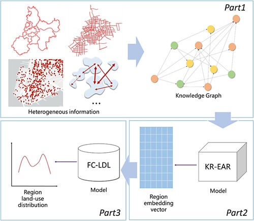
The overall framework of the approach is illustrated in Figure 1, which mainly consists of three parts:

• Constructing a KG. In this preparatory stage, a KG presenting POIs and other external factors for estimating the land-use distribution was constructed. The four selected kinds of heterogeneous information (POI semantic relations, spatial proximity between regions, road connectivity between regions, and administrative district relations) were transformed into entities and relations in the KG. The KG in our method was organized by multiple triplets and its entities were mainly composed of regions. The KG acts as the conjoint carrier of heterogeneous information and is intended to achieve the integration of heterogeneous information.

• Learning region representation. This stage involved determining the region representation by learning the latent semantic and geometric relationships in the KG. Specifically, the triplets in the KG constructed in the first stage were classified into entity-entity triples and entity-attribute triples and then input into a knowledge representation learning model (KR-EAR), which could separately model entity and attribute relations, encode them into a low-dimensional semantic space, and capture their correlations to obtain the region embedding vectors.

• Estimating land-use distributions. This final stage involved transforming the land-use distribution evaluation into a label distribution learning problem. The region embedding vectors generated in the second stage were mapped into the proportion of each land-use type in a region using an improved label distribution learning model (FC-LDL) by integrating label correlations, which were dynamically generated by the difference between label representations during training.

Figure 1. The overall framework of the proposed approach.

2.1. Constructing the KG

A KG can structurally organize complex and heterogeneous information together in a semantic network composed of multiple triplets $〈e_h,r,e_t〉$. Here, $e_h$ is the head entity, $e_t$ is the tail entity, and $r$ is the semantic relation between entities. A KG usually contains various types of entities and relations. According to different relations, the KG could be described as follows: (1) $G=\left(f_{r_1},f_{r_2},\cdots ,f_{r_{\mathrm{n}}}\right)$(1) Where $r_1,r_2,\cdots ,r_n$ are the relation types in $G$ and ${\mathrm{f}}_{r_n}$is the relation $r_n$ corresponding triplets.

As regional land-use distribution evaluation is usually performed by dividing an area into its basic elements, the main entities in our KG were the divided geographical cells. Considering the data acquisition and related factors that may affect the distribution of urban land use, the KG was designed using POI semantic relations, spatial proximity between regions, road connectivity between regions, and administrative districts relations (Figure 2). Nevertheless, the KG is not limited to these four factors and can be expanded as needed.

(a)

POI semantic triplets (${\mathrm{f}}_P$): POI is closely related to the land-use distribution of regions and is the main data source of the KG in our task. To retain as many POI semantics as possible, we defined ${\mathrm{f}}_P$ as: (2) ${\mathrm{f}}_P=〈e_{region},r_{category},e_{POI\mathrm{\_}fre}〉$(2)

Where the head entity $e_{region}$ is the divided geographical cell and the tail entity $e_{poi\mathrm{\_}fre}$ is the frequency of a POI category. The $r_{category}$ is the second-level POI category.

(b)

Spatial proximity triplets (${\mathrm{f}}_S$): According to the first law of geography (Tobler 1970), the closer regions are, the more likely they are to have similar land-use distributions. Therefore, we introduced spatial proximity to enhance the accuracy of land-use distribution evaluations. We defined ${\mathrm{f}}_S$ as: (3) ${\mathrm{f}}_S=〈e_{region},r_{nearby},e_{region}〉$(3)

Where the head entity $e_{region}$ and tail entity $e_{region}$ are both the divided geographical cells near each other.

(c)

Road connectivity triplets (${\mathrm{f}}_R$): The association between one region and another is not only affected by distance in a simple manner but also by the road connectivity between them. To capture the road connectivity between regions, we defined ${\mathrm{f}}_R$ as: (4) ${\mathrm{f}}_R=〈e_{region},r_{contain},e_{road}〉$(4)

Where the head entity $e_{region}$ is the divided geographical cells and the tail entity is roads. The $r_{contain}$ describes the content of regions and roads. When two regions contain the same road, this indicates a road connection between them. The more roads contained in both regions, the stronger the road connectivity between them.

(d)

Administrative districts triplets (${\mathrm{f}}_A$): The land-use distribution of the region has a certain correlation with the planning objectives of the administrative district where the region is located. For example, if the administrative district of the region is planned as a financial center, the financial enterprises tend to occupy the domain part of the region. Therefore, we considered the relationship between regions and administrative districts in the KG and defined ${\mathrm{f}}_S$ as: (5) ${\mathrm{f}}_A=〈e_{region},r_{belongsto},e_{district}〉$(5)

Where the head entity $e_{region}$ is the divided geographical cell and the tail entity $e_{district}$ is the administrative districts of the study area. The $r_{belongsto}$ describes the ownership of regions and districts.

2.2. Learning region representation

The goal of knowledge representation learning is to encode entities and relations into a low-dimensional semantic space and capture their correlations. Like most KGs, our KG has two types of triplets. One is an entity-entity triplet, in which the head and tail entities are both real objects, such as the triplets ${\mathrm{f}}_S$, ${\mathrm{f}}_R$, and ${\mathrm{f}}_A$ in Section 2.1. 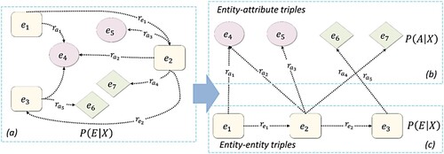The other is an entity-attribute triple, in which the tail entity is an abstract attribute, such as the triplet ${\mathrm{f}}_P$ in Section 2.1. However, current knowledge representation learning models usually treat all triplets as entity-entity triplets (Figure 3(a)) and neglect entity-attribute triplets which are the primary source of one-to-many and many-to-one relations. Hence, we used the KR-EAR (Lin, Liu, and Sun 2016), which can model entity relations and attribute relations separately (Figure 3(b) and (c)), to discover the semantic information between regions and external factors.

Figure 2. Part of the knowledge graph.

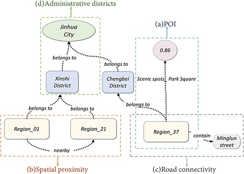
Figure 3. Illustrated graph of KR-EAR. (a) The entity-entity triples based-knowledge representation learning model. (b) and (c) The entity relation and attribute relation-based knowledge representation learning model.

We aimed to obtain the regional embedding representation $X$. In KR-EAR, the objective function is defined by maximizing the joint probability of entity-entity triplets $E$ and entity-attribute triplets $A$ given the embedding representation $X$: (6) $P\left(E,A|X\right)=P\left(E|X\right)P\left(A|X\right)$(6) (7) $=\prod _{〈e_h,r_e,e_t〉\in E}P\left(〈e_h,r_e,e_t〉\right|X)\prod _{〈e_h,r_a,a_t〉\in Y}P(〈e_h,r_a,a_t〉\left|X\right)$(7) Where $e_h$ indicates a set of regions $R=\left\{R_1,R_2,\cdots ,R_s\right\}$, $e_t$ indicates a set of geographic objects such as roads and districts, and $a_t$ indicates a set of POI frequencies $P=\left\{P_1,P_2,\cdots ,P_m\right\}$ in our KG. $P\left(〈e_h,r_e,e_t〉|X\right)$ indicates the conditional probability of the entity-entity triplets and $P\left(〈e_h,r_a,a_t〉\right|X)$ represents the conditional probability of entity-attribute triplets. The advantage of KR-EAR is that $P\left(〈e_h,r_e,e_t〉|X\right)$ and $P\left(〈e_h,r_a,a_t〉\right|X)$ are generated separately: $P\left(〈e_h,r_e,e_t〉|X\right)$ is generated by a common method, like TransE, and $P\left(〈e_h,r_a,a_t〉\right|X)$ is generated by a classification model. However, other models are calculated in the same way.

In this study, the conditional probability of the entity-entity triplets was generated based on TransE. As a simple and effective knowledge representation learning model, TransE has been proven to perform well in related tasks (Lin, Liu, and Sun 2016; Zhu et al. 2022). TransE is a distance-based model, which defines the distance between relations and entities in a triplet as a scoring function. $P\left(〈e_h,r_e,e_t〉|X\right)$ can be formulated as follows: (8) $P\left(〈e_h,r_e,e_t〉|X\right)={\displaystyle \frac{\mathrm{e}\mathrm{x}\mathrm{p}\left(g\left(〈e_h,r_e,e_t〉\right)\right)}{{\sum }_{\widehat{e_h}\in R}\mathrm{e}\mathrm{x}\mathrm{p}\left(g\left(〈\widehat{e_h},r_e,e_t〉\right)\right)}}$(8) (9) $g\left(〈e_h,r_e,e_t〉\right)=-||e_h+r_t-e_t|{|}_{L_1/L_2}+b_1$(9) where $g\left(\right)$ is the scoring function used to calculate the correlation between the relation $r_e$ and entity pair$〈e_h,e_t〉$, $b_1$ is a bias, and $L_1,L_2$ indicate the $L_1,L_2$ norm.

Furthermore, the correlation between entity and attribute can be suitably captured by a classification method while $P\left(〈e_h,r_a,a_t〉\right|X)$ can be formulated as follows: (10) $P\left(〈e_h,r_a,a_t〉|X\right)={\displaystyle \frac{\mathrm{e}\mathrm{x}\mathrm{p}\left(h\left(〈e_h,r_a,a_t〉\right)\right)}{{\sum }_{\widehat{a_t}\in P}\mathrm{e}\mathrm{x}\mathrm{p}\left(h\left(〈e_h,r_a,\widehat{a_t}〉\right)\right)}}$(10) (11) $h\left(〈e_h,r_a,a_t〉\right)=-\Vert f\left(e_h{W}_{r_a}+b_{r_a}\right)-E_{a_t}{\Vert }_{L_1/L_2}+b_2$(11) where $h\left(\right)$ is the scoring function for each attribute value of the entity, $f\left(\right)$ is an activate function such as ${\mathrm{t}\mathrm{a}\mathrm{n}}_h$, $E_{a_t}$ is the embedding vector of the attribute value, $W_{r_a}$ is a linear transformation, and $b_{r_a},b_2$ are biases.

2.3. Estimating land-use distributions

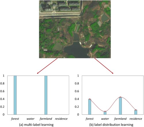
The challenge in predicting the proportion of each land-use type in a region is associated with the fact that each land-use type can be transformed into label distribution learning (LDL) (Geng 2016). LDL labels instances in a more natural way than multi-label learning and assigns a value to each possible label (Figure 4). In previous studies, to learn the distributions, Zhang et al. (2021) used an RF algorithm, while Huang et al. (2022) used an MLP model. We argue that they both consider the correlation between labels to a lesser extent, though there is a certain correlation between labels such as ‘forest’, ‘water’, and ‘farmland’ (Figure 4). Hence, we proposed an improved LDL model (FC-LDL) by integrating label correlations, in which the correlation was measured by the difference between label representations.

Figure 4. Distinction between multi-label learning and label distribution learning.

Based on our model, the problem could be formulated as follows: suppose $X=\left\{x_1,\cdots ,x_s\right\}$ is the embedding matrix of the study area, where $x\in {\mathbb{R}}^m$ and $m$ represents the dimension embedding vector of each region; the labels $L=\left\{l_1,\cdots ,l_q\right\}$ are a set of land-use types; the label distribution matrix $Y=\left\{y_1,\cdots ,y_s\right\}$ and $y=\left[p_{l_1},\cdots ,p_{l_q}\right]$ where $p\in \left[0,1\right]$ is the real proportion of each land-use type in a region and $\sum _{i=1}^q{p}_{l_i}=1$. Given a training set $S=\left\{X,Y\right\}=\left\{\left(x_1,y_1\right),\cdots ,\left(x_s,y_s\right)\right\}$, the goal is to model the relation between $X$ and $Y$.

Figure 5(a) shows the three steps involved in the operation of the FC-LDL model. First, we input the embedding matrix $X$ into an artificial neural network (ANN) shown in Figure 5(b) to obtain the initial predicted distribution $Y^{\sim }$. Second, we constructed a label correlation matrix $C$ to modify the initial predictions by multiplication. Finally, we input the output above into the softmax function to obtain predicted distributions with a sum of 1.

Figure 5. (a) Workflow of the FC-LDL, which is composed of an ANN, correlation matrix, and final predicted distribution. (b) Detailed demonstration of the two-layer ANN structure.

The core of our approach lies in how we defined the dependence of each label. The inverse-Euclidean distance is calculated to represent the correlation between labels: (12) $c\left(l_i,l_j\right)=-\sum _{k=1}^n\sqrt{{\left(p_{l_i}^k\right)}^2-{\left(p_{l_j}^k\right)}^2}$(12) where $c\left(l_i,l_j\right)$ is the correlation between label $l_i$ and $l_j$, $n$ is the amount of data in the training set, and $p_{l_i}^k$ is the proportion of label $l_i$ in the $k$^th record.

As Kullback-Leibler (KL) divergence can be used to measure the difference between probability distributions, KL divergence was selected as the loss function in FC-LDL, and the equation of KL divergence is shown in formula 14 in Section 3.2.

3. Experiments

3.1. Study area and data description

To verify the effectiveness of the proposed method and evaluate its prediction accuracy for the proportion of different land-use types, a case study was performed in Jinhua, in the central area of Changjiang River Delta, China. Jinhua is both a tourist attraction and an economic hinterland. Thus, reasonable urban planning is of great significance in Jinhua. We selected the prime part of Jinhua, shown in Figure 6(a), containing eleven administrative districts. For the region division problem, common methods such as traffic analysis zone (TAZ), regular grid, and irregular cells divided based on road network were applied in this study. However, since TAZ is generally provided by the government and is difficult to obtain, and regular grid has limitations in describing various urban morphology, we divided the study area into a three-level road network obtained from Open Street Map (www.openstreetmap.org) in 2022 (details shown in Table 1) and ultimately obtained the 350 regions shown in Figure 6(a). In the experiment, the POI dataset was collected from Amap (https://www.amap.com/) in 2020, which contained 222,226 records in 23 first-level categories and 267 s-level categories. In addition to the POI data and road networks, a land-use dataset obtained from the third national land-use survey of China containing 37 land-use types was utilized (Figure 6(b)). Apparently, the proportion of each regional type could constitute a 37-dimensional vector as the ground truth to participate in the training and evaluating process.

Figure 6. Study area. (a) Prime part of Jinhua, containing eleven administrative districts. (b) Real land-use distributions in the study area with 37 land-use types.

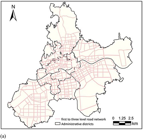
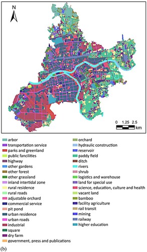
Table 1. Details of experimental road network.

Road level	OSM code	Numbers of roads
Primary	5113	269
Secondary	5114	718
Tertiary	5115	680

OSM code refers to the unified coding of road level in Open Street Map.

To prove that there was a correlation between land-use types, we took paddy field in Figure 6(b) as an example to calculate the average nearest distance (${\overline{d}}_{nearest}$) between it and the other 36 land-use types. The sorted results of ${\overline{d}}_{nearest}$ are shown in Figure 7 and the formula is as follows: (13) ${\overline{d}}_{nearest}={\displaystyle \frac{1}{n}\sum _{i=1}^n{d}_{nearest}^i\left(a,b\right)}$(13) where $n$ is the number of polygons of land-use type a and $d_{nearest}^i\left(a,b\right)$ is the nearest Euclidean distance between the ith polygon of land-use type a and the closest land-use type b polygon. Note that we used the center of the polygons when calculating the distance.

Figure 7. Average nearest distance (${\overline{d}}_{nearest}$) between paddy field and the other 36 land-use types.

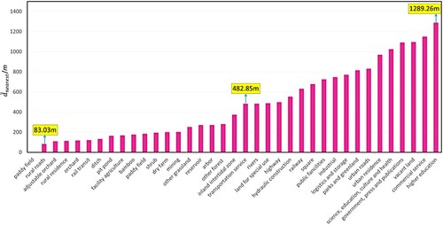
Figure 7 shows that the distribution of ${\overline{d}}_{nearest}$ between paddy fields and other land-use types varied significantly (the minimum was 83.03 m and the maximum was 1289.26 m) rather than being relatively smooth, indicating that there were significant differences in the spatial distribution between paddy fields and the other land-use types. It also revealed that the spatial distribution of paddy field was closer to the spatial distribution of rural and agricultural land-use types, such as rural roads, adjustable orchards, and rural residence than it was to urban land-use types, such as commercial service and higher education. In addition, to further prove the correlation between land-use types, we calculated the Pearson correlation between the proportion distribution of paddy field in the study area and that of adjustable orchards and commercial service. The Pearson correlation between paddy field and adjustable orchards showed a strong and significant positive correlation (r = 0.6437, p < 0.001) but that between paddy field and commercial service showed no significant correlation (r = 0.0895, p = 0.0942), further demonstrating that there were differences in correlation between land-use types.

3.2. Assessment metrics

In essence, the land-use distribution evaluation is a label distribution learning problem, which needs to evaluate the differences between the predicted distribution and the real distribution. Generally, most assessment metrics were based on distance as in previous studies. Cha (2007) analyzed many evaluation metrics to solve this problem, each of which has different connotations. Ultimately, we selected three representative metrics, KL divergence ($d_{kl}$), Cosine similarity ($c_{sim}$), and Chebyshev distance ($d_{cheb}$), to evaluate the accuracy of our proposed method.

1. KL divergence can measure the information loss of evaluated and real distributions by calculating the relative entropy. A smaller value indicates a better performance of the model. The formula is as follows: (14) $d_{kl}(\downarrow )=\sum _{i=1}^m{y}_i\mathrm{l}\mathrm{o}\mathrm{g}\left({\displaystyle \frac{\widehat{y_i}}{y_i}}\right)$(14)

2. Chebyshev distance represents the worst match between the evaluated and real distributions. A smaller value indicates a better performance of the model. The formula is as follows: (15) $d_{cheb}(\downarrow )=\mathrm{m}\mathrm{a}\mathrm{x}\left(\left|\widehat{y_i}-y_i\right|\right)$(15)

3. Cosine similarity reflects the similarity by calculating the cosine of the angle between evaluated and real distributions. A greater value indicates a better performance of the model. The formula is as follows: (16) $c_{sim}(\uparrow )={\displaystyle \frac{\left({\sum }_{i=1}^m\widehat{y_i}{y}_i\right)}{\left(\sqrt{{\sum }_{i=1}^m{\widehat{y_i}}^2}\sqrt{{\sum }_{i=1}^m{y}_i^2}\right)}}$(16) where $y_i$ is the real proportion of land-use type $i$ in a region, $\widehat{y_i}$ is the evaluated proportion of land-use type $i$ in a region, and $m$ is the number of land-use types.

In this study, to ensure the reliability of the estimated results, we calculated the average accuracy value from 10 random experimental repeats.

3.3. Baselines

We compared the proposed approach with the following representative baseline models to the effectiveness of this method. The comparison results are provided in Section 4.1.

1. Word2vec (Yao et al. 2017): This approach accounts for the factor of POI semantics. It treats POI categories as words and obtains POI embedding vectors through Word2vec. Subsequently, the region embedding vector is obtained by averaging POI vectors with weightings.

2. TF-IDF: This approach considers the importance of each POI category. We calculated the TF-IDF of each POI category in a region and formed them into a regional feature vector. For a fair comparison, this method considers second-level POI categories as our proposed approach does, by calculating the TF-IDF of the second-level POI categories.

3. TransE: The overall principle of this approach is similar to ours. The major difference is that all triplets are modeled the same way, whereas our method distinguishes entity-entity triplets and entity-attribute triplets and models them separately.

3.4. Implement details and parameter settings

As defined in Section 2.1, we regarded ${\mathrm{f}}_P$ as entity-attribute triplets, ${\mathrm{f}}_S$, ${\mathrm{f}}_R$, and ${\mathrm{f}}_A$ as entity-entity triplets, and ultimately obtained the number of experimental triplets as shown in Table 2. As in the region embedding process, the dimension of the generated vector is an important hyperparameter, therefore we conducted experiments to pick the most appropriate value for the hyperparameter from the following values: 50, 100, 150, 200, 250, 300, and 350. Table 3 shows the accuracy of the proposed method with different dimension settings, showing that our method performed best at an embedding dimension of 250.

Table 2. Details of experimental triples.

Dataset	Numbers
Region-entities	350
Attributes	603
Entity- entity triples	4912
Entity-attribute triples	9156

Table 3. Accuracy assessment of land-use distribution with different dimension settings.

Dimension	$d_{kl}(\downarrow )$	$d_{cheb}(\downarrow )$	$c_{sim}(\uparrow )$	Avg.rank
50	0.0358	0.4312	0.6774	6.3
100	0.0354	0.4350	0.6838	5.7
150	0.0306	0.3778	0.7403	3.7
200	0.0298	0.3727	0.7589	2.0
250	0.0277	0.3585	0.7766	1.0
300	0.0302	0.3784	0.7480	3.3
350	0.0312	0.4362	0.6820	6.0

The bold font indicates the best value in each assessment metric.

In the downstream learning model, 350 region embedding vectors were used as the inputs. The model was composed of two-layer ANNs, the hidden layer of it was set to 128 neurons. We set the ratio between the training and testing datasets to 4:1. The experiments were carried out in Windows 10/64 bit/i7. The proposed approach was implemented using Python in PyTorch, Numpy and Pandas. According to the relevant performance tests, the batch size was set to 32, the learning rate to 0.0005, and the epoch to 200.

Particularly, based on Section 2.3, a correlation matrix was constructed to enhance the learning process of evaluating land-use distribution. Here, the correlation threshold was another important hyperparameter that affected the precision. We investigated how the correlation threshold affects the results by setting the threshold $\alpha \ge$ 0, 0.2, 0.4, 0.6, or 0.8 and calculating the assessment metrics (Table 4). This revealed that our method performed best when the correlation threshold was set to $\alpha \ge$ 0.8.

Table 4. Accuracy assessment of land-use distribution with different correlation threshold settings.

Threshold $\left(\alpha \right)$	$d_{kl}(\downarrow )$	$d_{cheb}(\downarrow )$	$c_{sim}(\uparrow )$	Avg.rank
$\alpha \ge$0.8	0.0277	0.3585	0.7766	1.3
$\alpha \ge$ 0.6	0.0306	0.3613	0.7442	2.3
$\alpha \ge$ 0.4	0.0314	0.3689	0.7298	5.0
$\alpha \ge$0.2	0.0305	0.3520	0.7421	2.0
$\alpha \ge$0	0.0310	0.3640	0.7398	4.0

The bold font indicates the best value in each assessment metric.

4. Results and analysis

4.1. Performance of land-use distribution estimations

We evaluated the performance of two aspects of our method, the upstream region embedding methods and the downstream distribution learning methods, by comparing it with previous methods. Table 5 displays the accuracy of our method and the baselines. Both the MLP (Huang et al. 2022) and our FC-LDL proposed embedding methods displayed the regional features outstandingly. For FC-LDL, the KL divergence of our method was smaller than 0.03 while the cosine similarity was larger than 0.75, which indicates that the evaluated distribution is rather close to the ground truth. Additionally, the average Chebyshev distance was 0.3585; suggesting that the worst match between the evaluated distribution and ground truth is less than 0.36. For the baselines, as Word2vec and TF-IDF only considered the POI impact and ignore other factors, the precision was lower than that obtained by our model. However, it is worth mentioning that the simpler feature vectors constructed using TF-IDF performed better than those obtained using Word2vec, which indicates that the significance of each POI type has a stronger correlation with land-use type than the semantic of each POI type. Although TransE considered additional factors, similar to the proposed method, it was restricted in addressing the ‘many to many relations’ (Lin, Liu, and Sun 2016) in this task due to not modeling different types of relations separately, which further proves the necessity of our method.

Table 5. Comparison with other representative methods.

Embedding method	Distribution learning model	$d_{kl}(\downarrow )$	$d_{cheb}(\downarrow )$	$c_{sim}(\uparrow )$	Avg.rank
Proposed	MLP	0.0328	0.4286	0.7157	1.0
Word2vec		0.0356	0.4444	0.6689	3.0
TF-IDF		0.0342	0.4428	0.6755	2.0
TransE		0.0363	0.4532	0.6541	4.0
Proposed	FC-LDL (proposed)	0.0277	0.3585	0.7766	1.0
Word2vec		0.0322	0.3663	0.7284	3.0
TF-IDF		0.0327	0.3622	0.7363	2.0
TransE		0.0360	0.4328	0.6634	4.0

The bold font indicates the best value in each assessment metric.

Furthermore, the proposed distribution learning model (FC-LDL) achieved a higher accuracy than that obtained with MLP for all embedding methods. As with FC-LDL, MLP is composed of a two-layered ANN; however, the improved performance of FC-LDL over MLP is due to consideration of the correlation between labels by adding a module to dynamically create a label correlation matrix, which enhances the outputs.

4.2. Influence analysis of the selected factors

As mentioned in Section 2.1, four factors (POI, spatial proximity, road connectivity, and administrative districts) were considered in this study. To determine whether these factors contribute to the accuracy of our predictions, we built the KG with different fusion schemes and compared their performance. Among them, the training data points for ${\mathrm{f}}_{\mathrm{A}}$ were fewer; thus, ${\mathrm{f}}_{\mathrm{A}}$ could hardly be trained alone. The results are shown in Table 6. Performance is ranked as follows: ${\mathrm{f}}_{\mathrm{P}}+{\mathrm{f}}_{\mathrm{A}}+{\mathrm{f}}_{\mathrm{S}}+{\mathrm{f}}_{\mathrm{R}}$ (ours) > ${\mathrm{f}}_{\mathrm{P}}+{\mathrm{f}}_{\mathrm{S}}$ > ${\mathrm{f}}_{\mathrm{P}}$ > ${\mathrm{f}}_{\mathrm{P}}+{\mathrm{f}}_{\mathrm{R}}$. Our results imply that the combination of the four factors achieved the best performance; thus, demonstrating that the knowledge fusion mode is superior to the single-factor mode. Second, by comparing ${\mathrm{f}}_{\mathrm{P}}$ and ${\mathrm{f}}_{\mathrm{P}}+{\mathrm{f}}_{\mathrm{S}}$, we discovered that the accuracy of the latter KG improved significantly, which indicates that the spatially adjacent regions are more likely to have similar land-use distribution. Last, by comparing ${\mathrm{f}}_{\mathrm{P}}$ and ${\mathrm{f}}_{\mathrm{P}}+{\mathrm{f}}_{\mathrm{R}}$, we observed that the fusion of ${\mathrm{f}}_{\mathrm{R}}$ reduces accuracy rather than improving it. Numerous studies proposing models for traffic flow prediction (Zhao et al. 2019) and human mobility prediction (Li et al. 2021a, 2021b) may be more accurate after considering road connectivity; however, in our study, road connectivity was slightly negatively correlated with land-use distribution. Considering road connectivity overcomes the limitation of distance and increases the connection between non-adjacent areas. In the past, insufficient transportation resulted in less distance between living and working places. However, for regions that are relatively far apart but have convenient transportation (A and B), people can choose to work in region A and live in region B. In such instances, strong road connectivity contributes to more differentiated land-use distribution. Furthermore, ${\mathrm{f}}_{\mathrm{P}}$ > ${\mathrm{f}}_{\mathrm{P}}+{\mathrm{f}}_{\mathrm{R}}$ also revealed that the prediction accuracy is not number-of-factor dependent. It should be noted that verifying the correlation of each factor to the downstream tasks is essential before constructing the KG.

Table 6. Accuracy assessment of land-use distribution with different fusion schemes.

Factors	$d_{kl}(\downarrow )$	$d_{cheb}(\downarrow )$	$c_{sim}(\uparrow )$	Avg.rank
${\mathrm{f}}_{\mathrm{P}}$	0.0343	0.4269	0.6766	3.3
${\mathrm{f}}_{\mathrm{P}}+{\mathrm{f}}_{\mathrm{A}}$	–	–	–	–
${\mathrm{f}}_{\mathrm{P}}+{\mathrm{f}}_{\mathrm{S}}$	0.0315	0.3735	0.7510	2.0
${\mathrm{f}}_{\mathrm{P}}+{\mathrm{f}}_{\mathrm{R}}$	0.0354	0.4429	0.6802	3.7
${\mathrm{f}}_{\mathrm{P}}+{\mathrm{f}}_{\mathrm{A}}+{\mathrm{f}}_{\mathrm{S}}+{\mathrm{f}}_{\mathrm{R}}$(ours)	0.0277	0.3585	0.7766	1.0

The bold font indicates the best value in each assessment metric.

4.3. Influence analysis of the granularity of land-use classification

Previous studies focused on unique land-use classification and rarely explored the impact of different land-use classifications on the assessment accuracy. As described in Section 4.1, the land-use classification directly determines the distribution of ground truth. The original data included in this study were characterized by a fine classification granularity of land-use types, including 37 land-use types; thus, indicating a proclivity for two main problems: First, the distribution of ground truth will be sparse. Second, the proportion of each type will be decreased; hence, the distribution of the true value will tend to be smoother than that of larger classification granularities. Therefore, we conducted a comparative experiment to explore the influence of the land-use classification granularity on accuracy. We re-classified the 37 land-use types into 13 land-use types with references to the relevant land-use classification standards (Figure 8) (Lv et al. 2022) and compared the estimated accuracy of each land-use classification. The results are shown in Table 7. We discovered that when the number of land-use classifications was aggregated from 37 to 13, our method achieved higher accuracy on the cosine similarity and the average Chebyshev distance. Particularly, the cosine similarity was larger than 0.80 for large classification granularity, which indicates that the evaluated distribution is relatively close to the ground truth. We believe that the large classification granularity broadens the value range of each type, makes the distribution fluctuate significantly, and strengthens the feature extraction during model training. Nevertheless, the KL divergence with large classification granularity is not ideal. We observed that the KL divergence was affected by the dimension of ground truth (Xu et al. 2016). Thus, the KL divergence is irrational to measure the accuracy when the ground truth dimension changes.

Figure 8. Integration of the 37 land-use types into 13 land-use types.

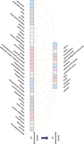
Table 7. Accuracy assessment of land-use distribution with different granularity of land-use classification.

Dimension	$d_{kl}(\downarrow )$	$d_{cheb}(\downarrow )$	$c_{sim}(\uparrow )$	Avg.rank
37	0.0277	0.3585	0.7766	1.7
13	0.0548	0.3466	0.8013	1.3

The bold font indicates the best value in each assessment metric.

4.4. Error analysis

The error analysis assessed two aspects. First, we performed a quantitative analysis of the errors on each land-use type in the evaluation results. Subsequently, we analyzed the errors caused by the input information and visualized three representative regions with large errors for demonstration.

4.4.1. Errors on each land-use type

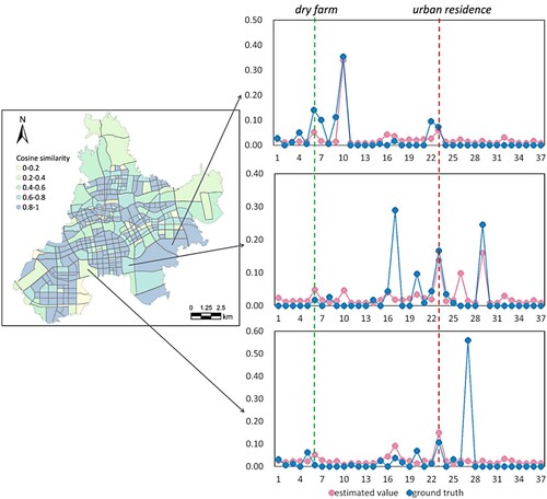
In Figure 9, we visualized the ground truth and the estimated results of three regions at different cosine similarity levels and discovered that the estimated value of some fixed land-use types was adequate (e.g. urban residence, corresponding to the red line in Figure 9), while that of others was not (e.g. dry farm, corresponding to the green line in Figure 9). Next, we extracted the land-use types where small and large errors occurred. As the proportion of land-use types in the study area differed greatly, we calculated the relative error using the following formula to measure the accuracy of the land-use types: (16) ${\delta }_c(\downarrow )={\displaystyle \frac{{\sum }_{i=1}^n\left(\left|\widehat{y_i}-y_i\right|\right)}{{\sum }_{i=1}^n{y}_i}}$(16) Where $y_i$ is the real proportion of land-use type $c$ in region $i$, $\widehat{y_i}$ is the evaluated proportion of land-use type $c$ in region $i$, and $n$ is the number of regions in the study area.

Figure 9. Visualization of the ground truth and the estimated results of three typical regions with different cosine similarity levels. The left panel represents the visualization of the cosine similarity in the study area and the right panel represents the visualization of the ground truth and the estimated value.

The results of the land-use type error analysis are presented in Table 8. Most errors had a value lower than 4, which indicates that our approach performed adequately in most land-use types. Specifically, we observed that our approach performed relatively better in the urban residence and industrial types than in other types. Furthermore, the performance decreased drastically in the rail transit and rural road types. We hypothesize that there are two main reasons for such a phenomenon: the relatively small proportion of this land-use type, which makes it challenging to capture the required characteristics, and the omission of rail transit and rural roads in the KG construction process (we selected only first to third-level road networks). As this is not the only conjecture that leads to differences in accuracy among different categories, the following section further discusses possible sources of errors.

Table 8. Errors in each land-use type.

ID	Land-use types	Proportion of land-use types(%)	${\delta }_c(\downarrow )$	Rank
23	Urban residence	0.2068	0.4953	1
17	Industrial	0.1441	0.6575	2
10	Paddy field	0.1568	1.1665	3
3	Other forests	0.0177	1.2036	4
7	Orchard	0.0367	1.2204	5
15	Highway	0.0127	1.2352	6
4	Rural residence	0.0319	1.2553	7
5	Pit pond	0.0170	1.3426	8
29	Rivers	0.0446	1.3995	9
6	Dry farm	0.0533	1.4058	10
22	Commercial service	0.0278	1.4304	11
24	Urban roads	0.0065	1.4408	12
25	Science, education, culture, and health	0.0312	1.4727	13
20	Parks and greenland	0.0350	1.5182	14
18	Land for special use	0.0147	1.5212	15
26	Government, press, and publications	0.0078	1.5568	16
16	Other grasslands	0.0203	1.6017	17
32	Railway	0.0223	1.6308	18
33	Logistics and warehouse	0.0036	1.6914	19
2	Other gardens	0.0097	1.7016	20
1	Arbor	0.0436	1.7317	21
8	Hydraulic construction	0.0060	1.8167	22
19	Transportation service	0.0062	1.8711	23
21	Public facilities	0.0047	1.9515	24
27	Higher education	0.0196	2.3814	25
9	Reservoir	0.0087	2.8154	26
36	Square	0.0006	3.1528	27
34	Inland intertidal zone	0.0029	4.8116	28
14	Mining	0.0027	4.9154	29
30	Facility agriculture	0.0008	12.3425	30
37	Vacant land	0.0002	19.0166	31
13	Bamboo	0.0011	22.3553	32
11	Pit pond	0.0005	22.4190	33
12	Shrub	0.0008	22.4829	34
28	Adjustable orchard	0.0004	27.8171	35
31	Rail transit	0.0005	57.3299	36
35	Rural roads	0.0003	66.6771	37

4.4.2. Source of errors

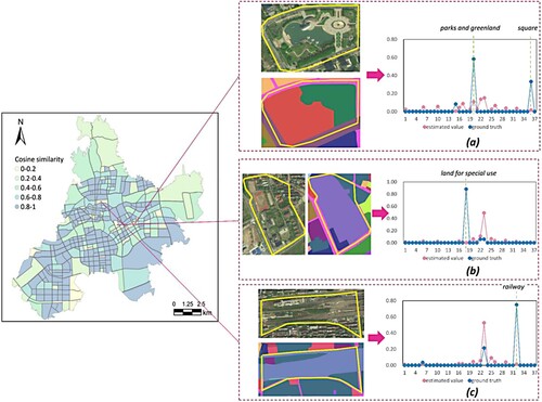
Previous sections have adequately discussed the influence of the different parameters on the proposed model. In this section, we overlook the internal factors of the model and only consider the impact of external input on evaluation accuracy. To explain the main source of errors, we visualized three representative regions with large errors in Figure 10. The reasons are summarized as follows:

• Inconsistent description between input information and ground truth. In Figure 10(a), the proportion of square is 0.33, while our model only assigns 0.01 to it. By analyzing the input POIs, we discovered that there is no category called square in the POIs and the category of square related POIs are defined as park rather than square. This shows inconsistencies between the input information descriptions and the ground truth can lead to large errors in some categories.

• Equal weight input of dominant information. The region exhibited in Figure 10(a) mainly consists of parks and greenland (proportion = 0.58). However, the estimated proportion of parks and greenland was only 0.11. Parks and greenland was the dominant land-use type in the region with only 2 related POIs, accounting for 1% of the total dataset. In this study, as the original information was input into the model in an equally weighted manner, this will hinder highly significant information with a low presence to play a decisive role.

• Lacking relevant input information. The region exhibited in Figure 10(b) is mainly for special use (proportion = 0.88). Contrary to expectations, the estimated proportion of land for special use was 0. After a thorough investigation, we observed that land for special use refers to places requiring confidentiality or special protection, such as military facilities and religions. Hence, it is difficult to collect information related to these places through open data sources.

• Incomplete input information. The region exhibited in Figure 10(c) mainly consists of railway (proportion = 0.75). However, our model only assigned 0.02 to this region. The reason for this phenomenon is that we filtered out the railway-related information when preprocessing the original data, and only the main roads (level 1–3) were selected. Nevertheless, we believe that given complete data, we will obtain more accurate results.

Figure 10. Three representative regions with large errors caused by the input information.

5. Conclusion

In this study, we first addressed the issue of neglecting correlations between land-use type and numerous external factors including POIs. To address this, we designed a KG to bear POIs and other related heterogeneous data, utilizing a knowledge embedding model to directly obtain the region embedding vectors by learning the complex and implicit relations, and mapped the region embedding vectors to the land-use distributions using a label distribution learning method with integrating correlations between land-use types. Further, we conducted a thorough experiment in Jinhua, China. The experimental results demonstrated the superiority of the proposed method compared to previously used methods.

In our experiment, we confirmed that estimating land-use distribution in a knowledge fusion manner achieved better performance than using single POIs, especially when fusing the spatial distance between regions. Meanwhile, we provided a flexible solution for the incorporation of numerous related factors, which could allow for the appropriate expansion with additional data. Furthermore, the proposed method generated region embedding vectors directly by learning the comprehensive semantics and relations in a KG instead of indirectly by aggregating POI vectors (Yao et al. 2017; Huang et al. 2022), which decreased the complexity of the model and improved its efficiency.

We corroborated previous reports supporting the dominance of POIs in sensing land-use distribution, as using POI category semantic information alone led to adequate estimations. In this paper, the proposed approach organized the POI information into two modes (category semantics and quantity), which could be used to thoroughly investigate the co-occurrence relationships and quantitative characteristics of POIs. Nevertheless, the expressiveness of POIs remains limited (Huang et al. 2022). We showed that it is of vital importance to supplement POIs with information on external factors (as in our proposed method).

Previous studies generally treated land-use types independently when estimating land-use distributions (Yan et al. 2017; Yao et al. 2017; Huang et al. 2022), which does not accurately represent the real-life situation. To this end, we proposed an innovative estimation model that uses the dynamic calculation of correlations between land-use types from training data in the land-use distribution learning process. Our results showed that considering the correlation between land-use types leads to better estimates than those from models that do not consider it.

Future work could be conducted in three directions. First, to illustrate and simplify the approach by quantifying the contributions of each factor to the model. In this way, fusing irrelevant and contradictory factors in the model, such as road connectivity, which was subjective in this study, could be avoided. Second, the proposed method could perform more effectively when more data was available; thus, we would like to integrate more relevant data, such as policy texts and area of interest data. Last, temporal dynamics, which are an important factor in land-use distribution studies (Zhu et al. 2022), should be further considered to enhance the land-use labeling mechanism.

Author contributions

Jing Li and Haiyan Liu conceived this study. Jing Li designed the methodology and Jia Li implemented the main model. Xiaohui Chen illustrated the main figures. Zekun Tao aided in the interpretation of the results. All authors have read and agreed to the published version of the manuscript.

Acknowledgments

The authors thank the editors and anonymous reviewers for their insightful comments and constructive suggestions.

Disclosure statement

No potential conflict of interest was reported by the author(s).

Data availability statement

Open-source data is available in public repositories. The road network can be obtained from Open Street Map (www.openstreetmap.org), the POI dataset can be obtained from Amap (https://www.amap.com/), and the POI classification information can be obtained from https://lbs.amap.com/api/webservice/download. However, the land-use distribution dataset is not available due to its confidentiality.

Additional information

Funding

This work was supported by National Natural Science Foundation of China [grant number 41801313].

References

- Andrade, Renato, Ana Alves, and Carlos Bento. 2020. “POI Mining for Land Use Classification: A Case Study.” ISPRS International Journal of Geo-Information 9 (9): 493. doi:10.3390/ijgi9090493.
- Andris, Clio. 2016. “Integrating Social Network Data Into GISystems.” International Journal of Geographical Information Science 30 (10): 1–23. doi:10.1080/13658816.2016.1153103.
- Bayer, Markus, Marc-André Kaufhold, and Christian Reuter. 2022. “A Survey on Data Augmentation for Text Classification.” ACM Computing Surveys 55 (7): 1–39. doi:10.1145/3544558.
- Bengio, Yoshua, Aaron Courville, and Vincent Pascal. 2013. “Representation Learning: A Review and New perspectives.” IEEE Transactions on Pattern Analysis and Machine Intelligence 35 (8): 1798–1828. doi:10.1109/TPAMI.2013.50.
- Burton, E., M. Jenks, and K. Williams. 2003. The Compact City: A Sustainable Urban Form? London, England: Routledge. doi:10.4324/9780203362372.
- Cha, Sung-Huyk. 2007. “Comprehensive Survey on Distance/Similarity Measures between Probability Density Functions.” International Journal of Mathematical Models and Methods in Applied Sciences 1 (4): 300–307.
- Gao, Song, Janowicz Krzysztof, and Couclelis Helen. 2017. “Extracting Urban Functional Regions from Points of Interest and Human Activities on Location-Based Social Networks.” Transactions in GIS 21 (3): 446–467. doi: 10.1111/tgis.12289.
- Geng, Xin. 2016. “Label Distribution Learning.” IEEE Transactions on Knowledge and Data Engineering 28 (7): 1734–1748. doi: 10.1109/TKDE.2016.2545658.
- Han, Haoying, Xiang Yu, and Ying Long. 2016. “Identifying Urban Functional Zones Using Bus Smart Card Data and Points of Interest in Beijing.” City Planning Review 116 (6): 193–217. doi: 10.1007/978-3-319-19342-7_10.
- Hoffmann, Raphael, Congle Zhang, Xiao Ling, Luke Zettlemoyer, and Daniel S. Weld. 2011. “Knowledge-Based Weak Supervision for Information Extraction of Overlapping Relations.” In Proceedings of the 49th Annual Meeting of the Association for Computational Linguistics: Human Language Technologies-Volume 1, 541–550. Portland: ACL.
- Hong, Danfeng, Lianru Gao, Naoto Yokoya, Jing Yao, Jocelyn Chanussot, Qian Du, and Bing Zhang. 2021. “More Diverse Means Better: Multimodal Deep Learning Meets Remote-Sensing Imagery Classification.” IEEE Transactions on Geoscience and Remote Sensing 59 (5): 4340–4354. doi:10.1109/TGRS.2020.3016820
- Huang, Weiming, Lizhen Cui, Meng Chen, Daokun Zhang, and Yao Yao. 2022. “Estimating Urban Functional Distributions with Semantics Preserved POI Embedding.” International Journal of Geographical Information Science 36 (10): 1905–1930. doi:10.1080/13658816.2022.2040510.
- Jiang, Shan, Ana Alves, Rodrigues Filipe, Joseph Ferreira Jr., and Francisco C. Pereira. 2015. “Mining Point-of-Interest Data from Social Networks for Urban Land Use Classification and Disaggregation.” Computers, Environment and Urban Systems 53 (9): 36–46. doi:10.1016/j.compenvurbsys.2014.12.001.
- Jiang, Bingchuan, Gang Wan, Jian Xu, Feng Li, and Huiqi Wen. 2018. “Geographic Knowledge Graph Building Extracted from Multi-Sourced Heterogeneous Data.” Acta Geodaetica et Cartographica Sinica 47 (8): 1051–1061. doi:10.11947/j.AGCS.2018.20180113.
- Kasneci, Gjergji, Fabian M. Suchanek, Georgiana Ifrim, Maya Ramanath, and Gerhard Weikum. 2008. “Naga: Searching and Ranking Knowledge.” In 2008 IEEE 24th International Conference on Data Engineering, 953–962. Cancun: IEEE. doi:10.1109/ICDE.2008.4497504.
- Li, Mingxiao, Song Gao, Feng Lu, Kang Liu, Hengcai Zhang, and Wei Tu. 2021a. “Prediction of Human Activity Intensity Using the Interactions in Physical and Social Spaces Through Graph Convolutional Networks.” International Journal of Geographical Information Science 35 (12): 2489–2516. doi: 10.1080/13658816.2021.1912347.
- Li, Jing, Haiyan Liu, Wenyue Guo, and Xin Chen. 2021b. “A Spatio-Temporal Network for Human Activity Prediction Based on Deep Learning.” Acta Geodaetica et Cartographica Sinica 50 (4): 522–531 doi:10.11947/j.AGCS.2021.20200230.
- Lin, Yankai, Zhiyuan Liu, and Maosong Sun. 2016. “Knowledge Representation Learning with Entities, Attributes and Relations.” In Proceedings of the 25th International Joint Conference on Artificial Intelligence, 2866–2872. New York: ACM. doi:10.1109/LSP.2016.2537376.
- Lv, Yuxia, Yuxian Zhang, Chongli Ma, Ying Zhang, and Tang Yin. 2022. “Land Use Classification Comparative Analysis between IPCC and China.” Geospatial Information 20 (7): 22–25. 1672-4623.2022.07.005. doi:10.3969/j.issn.
- Ma, Qiang, Liangxu Wang, Xin Gong, and Ke Li. 2022. “Research on the Rationality of Public Toilets Spatial Layout Based on the POI Data from the Perspective of Urban Functional Area.” [In Chinese.] Geographic Information Sciences 24 (01): 50–62. doi:10.12082/dqxxkx.2022.210331.
- Niu, Ning, Xiaoping Liu, He Jin, Xinyue Ye, Yu Liu, Xia Li, Yimin Chen, and Shaoying Li. 2017. “Integrating Multi-Source Big Data to Infer Building Functions.” International Journal of Geographical Information Science 31 (9): 1871–1890. doi:10.1080/13658816.2017.1325489.
- Portnov, Boris A., and Moshe Schwart. 2009. “Urban Clusters as Growth Foci.” Journal of Regional Science 49 (2): 287–310. doi: 10.1111/j.1467-9787.2008.00587.x.
- Ren, Tingting, Xiuyi Jia, Weiwei Li, Lei Chen, and Zechao Li. 2019. “Label Distribution Learning with Label Correlations Via Low-Rank Approximation.” In Proceedings of the 28th International Joint Conference on Artificial Intelligence, 3325–3331. Macao: AAAI. doi:10.1002/int.22307.
- Tian, Li, and Tiyan Shen. 2011. “Evaluation of Plan Implementation in the Transitional China: A Case of Guangzhou City Master Plan.” Cities 28 (1): 11–27. doi: 10.1016/j.cities.2010.07.002.
- Tobler, W. R. 1970. “A Computer Movie Simulating Urban Growth in the Detroit Region.” Economic Geography 46 (sup. 1): 234–240. doi:10.2307/143141.
- Tu, Wei, Jinzhou Cao, Yang Yue, Shih-Lung Shaw, Meng Zhou, Zhensheng Wang, Xiaomeng Chang, Yang Xu, and Qingquan Li. 2017. “Coupling Mobile Phone and Social Media Data: A New Approach to Understanding Urban Functions and Diurnal Patterns.” International Journal of Geographical Information Science 31 (12): 2331–2358. doi: 10.1080/13658816.2017.1356464.
- Wang, Minghua, Qiang Wang, Danfeng Hong, Swalpa Kumar Roy, and Jocelyn Chanussot. 2022. “Learning Tensor Low-Rank Representation for Hyperspectral Anomaly Detection.” IEEE Transactions on Cybernetics 53 (1): 679–691. doi:10.1109/TCYB.2022.3175771.
- Wang, Bihui, Yunchao Wu, and Xiaochun Wu. 2012. ��Urban Land Use Classification Using High Resolution Remote Sensing Data.” [In Chinese.] Remote Sensing Information 27 (4): 111–115. doi:10.3969/j.issn.1000-3177.2012.04.020.
- Wu, Lun, Ximeng Cheng, Di Zhu Chaogui Kang, Zhou Huang, and Yu Liu. 2018. “A Framework for Mixed-Use Decomposition Based on Temporal Activity Signatures Extracted from Big Geo-Data.” International Journal of Digital Earth 13 (6): 708–726. doi:10.1080/17538947.2018.1556353.
- Xu, Kun, Siva Reddy, Yansong Feng, Songfang Huang, and Dongyan Zhao. 2016. “Question Answering on Freebase Via Relation Extraction and Textual Evidence.” In Proceedings of the 54th Annual Meeting of the Association for Computational Linguistics, 2326–2336. Berlin: ACL. doi:10.18653/v1/P16-1220.
- Yan, Bo, Krzysztof Janowicz, Gengchen Mai, and Song Gao. 2017. “From ITDL to Place2Vec: Reasoning about Place Type Similarity and Relatedness by Learning Embeddings from Augmented Spatial Contexts.” In Proceedings of the 25th ACM SIGSPATIAL International Conference on Advances in Geographic Information Systems, 1–10. Redondo Beach: ACM. doi:10.1145/3139958.3140054.
- Yang, Donghua, Tao He, Hongzhi Wang, and Jinbao Wang. 2022. “Survey on Knowledge Graph Embedding Learning.” [In Chinese.] Journal of Software 33 (9): 3370–3390. doi: 10.13328/j.cnki.jos.006426.
- Yao, Yao, Xia Li, Xiaoping Liu, Penghua Liu, Zhaotang Liang, Jinbao Zhang, and Ke Mai. 2017. “Sensing Spatial Distribution of Urban Land use by Integrating Points-of-Interest and Google Word2Vec model.” International Journal of Geographical Information Science 31 (4): 825–848. doi: 10.1080/13658816.2016.1244608.
- Yuan, Jing, Yu Zheng, and Xing Xie. 2012. “Discovering Regions of Different Functions in a City Using Human Mobility and POIs.” In Proceedings of the 18th ACM SIGKDD International Conference on Knowledge Discovery and Data Mining, 186–194. Long Beach: ACM.
- Yue, Yang, Yan Zhuang, Anthony G. O. Yeh, Jinyun Xie, Chenglin Ma, and Qingquan Li. 2017. “Measurements of POI-Based Mixed Use and their Relationships with Neighbourhood Vibrancy.” International Journal of Geographical Information Science 31 (4): 658–675. doi: 10.1080/13658816.2016.1220561.
- Zhang, Jinbao, Xia Li, Yao Yao, Ye Hong, Jialyu He, Zhangwei Jiang, and Jianchao Sun. 2021. “The Traj2Vec Model to Quantify Residents’ Spatial Trajectories and Estimate the Proportions of Urban Land-Use Types.” International Journal of Geographical Information Science 35 (1): 193–211. doi: 10.1080/13658816.2020.1726923.
- Zhao, Ling, Yujiao Song, Chao Zhang, Yu Liu, Pu Wang, Tao Lin, Min Deng, and Haifeng Li. 2019. “T-GCN: A Temporal Graph Convolutional Network for Traffic Prediction.” IEEE Transactions on Intelligent Transportation Systems 21 (9): 3848–3858. doi: 10.1109/TITS.2019.2935152.
- Zheng, Yu, Capra Licia, Wolfson Ouri, and Yang Hai. 2014. “Urban Computing: Concepts, Methodologies, and Applications.” ACM Transaction on Intelligent Systems and Technology 5 (3): 38.1–38.55. doi:10.1145/2629592.
- Zheng, Zhijian, Rongbao Zheng, Jiayuan Xu, and Jiaqiu Wang. 2020. “Identification of Urban Functional Regions Based on POI Data and Place2vec Model.” [In Chinese.] Geography and Geo-Information Science 36 (04): 48–56. doi: 10.3969/j.issn.1672-0504.2020.04.008.
- Zhou, Hang, and Hong Fan. 2022. “Research on the Identification of Urban Function Areas and the Hot Spots Based on Crowdsourcing Geographic data.” [In Chinese.] Engineering Journal of Wuhan University 55 (04): 417–426. doi:10.14188/j.1671-8844.2022-04-013.
- Zhou, Ying, Hui Xue, and Xing Geng. 2015. “Emotion Distribution Recognition from Facial Expressions.” In Proceedings of the 23rd ACM International Conference on Multimedia, 1247–1250. Brisbane: ACM. doi:10.1145/2733373.2806328.
- Zhu, Jiawei, Xin Han, Hanhan Deng, Chao Tao, and Haifeng Li. 2022. “KST-GCN: A Knowledge-Driven Spatial-Temporal Graph Convolutional Network for Traffic Forecasting.” IEEE Transactions on Intelligent Transportation Systems 23 (9): 15055–15065. doi:10.1109/TITS.2021.3136287.