A scalable software package for time series reconstruction of remote sensing datasets on the Google Earth Engine platform

ABSTRACT

Spatiotemporal residual noise in terrestrial earth observation products, often caused by unfavorable atmospheric conditions, impedes their broad applications. Most users prefer to use gap-filled remote sensing products with time series reconstruction (TSR) algorithms. Applying currently available implementations of TSR to large-volume datasets is time-consuming and challenging for non-professional users with limited computation or storage resources. This study introduces a new open-source software package entitled ‘HANTS-GEE’ that implements a well-known and robust TSR algorithm, i.e. Harmonic ANalysis of Time Series (HANTS), on the Google Earth Engine (GEE) platform for scalable reconstruction of terrestrial earth observation data. Reconstruction tasks can be conducted on user-defined spatiotemporal extents when raw datasets are available on GEE. According to site-based and regional-based case evaluation, the new tool can effectively eliminate cloud contamination in the time series of earth observation data. Compared with traditional PC-based HANTS implementation, the HANTS-GEE provides quite consistent reconstruction results for most terrestrial vegetated sites. The HANTS-GEE can provide scalable reconstruction services with accelerated processing speed and reduced internet data transmission volume, promoting algorithm usage by much broader user communities. To our knowledge, the software package is the first tool to support full-stack TSR processing for popular open-access satellite sensors on cloud platforms.

KEYWORDS:

• Time series reconstruction
• remote sensing
• Google Earth Engine
• HANTS
• gap-filling

1. Introduction

Long-term archived remote sensing datasets collected by satellite missions such as AVHRR (Advanced Very High-Resolution Radiometer), Landsat, Sentinel, and MODIS (Moderate Resolution Imaging Spectroradiometer) provided unprecedented opportunities for earth system science research and global ecosystem monitoring (Bretherton 1985; Reichstein et al. 2019; Shiklomanov et al. 2019; Steffen et al. 2020; Yu et al. 2022a). However, satellite-based land surface observations, especially by optical or thermal sensors, are often contaminated by different sources of noise such as clouds, shadows, aerosol, and observational geometry (Holben 1986; Zhou et al. 2021). Many data processing strategies have been designed to eliminate the effect of contaminated observations on downstream applications (Shen et al. 2015). For some remote sensing products, most contaminated observations can be correctly identified by strict quality control (QC) procedures (Zhu and Woodcock 2012) and are excluded in further analysis, resulting in gaps in the dataset. Because of limited spectral bands and complex noise sources, both omission or commission errors still existed in quality control procedures, which leaves residual contaminated observations in a dataset, or some valid observations are masked out (Zhou et al. 2021). For sensors with very dense observations (e.g. daily for MODIS), the derived land surface products (e.g. vegetation index) commonly used the temporal compositing method to remove noisy observations by assuming that noise appears as a fast disturbance compared with the slower evolution of land surface conditions (Holben 1986). Residual contaminated observations can still exist after the temporal compositing processing as continuous cloudy-sky may last longer than selected temporal compositing windows (Roerink, Menenti, and Verhoef 2000; Zhou, Jia, and Menenti 2015).

To further fill the gaps and eliminate the impact of residual contaminated observations, a panoply of time series reconstruction (TSR) algorithms has been proposed in past decades by interpolating values of gapped position based on valid observations within a temporal window (Hird and McDermid 2009; Geng et al. 2014; Zhou et al. 2016a; Li et al. 2021). According to the principle of missing information restoration, Li et al. (2021) categorized these methods as temporal-based methods, frequency-based methods, and hybrid methods. Temporal methods such as MVC (Holben 1986), Savitzky–Golay (SG) filter (Chen et al. 2004), Asymmetric Gaussian (AG) function fitting (Jonsson and Eklundh 2002), and Double Logistic (DL) function fitting (Beck et al. 2006; Yang et al. 2019) reconstruct noisy time series based on temporally neighbor observations or phenological characteristics of vegetation, which can capture local detail variation well (Zhou et al. 2016a). In contrast, frequency-based methods including Fourier analysis (Menenti et al. 1993), Harmonic ANalysis of Time Series (HANTS) (Roerink, Menenti, and Verhoef 2000) and wavelet transform (WT) (Lu et al. 2007) assume noisy observations always present as high frequency components in time series. The methods mainly eliminate the impact of noisy observations by decomposing time series into sub-signals into different frequencies and removing high-frequency components. Both the temporal-based methods and frequency-based methods only consider temporal continuity while ignoring spatial correlation of time series. Hybrid methods combine both spatial and temporal information together for image reconstruction. All the Temporal Spatial filter (TSF) (Fang et al. 2008), Search and Fill Algorithm with Moving Offset Method (SFA-MOM) (Padhee and Dutta 2019), Spatio-Temporal Savitzky–Golay (STSG) method (Cao et al. 2018) and Spatio-Temporal Tensor completion (ST-Tensor) method (Chu et al. 2021) belong to this category. Most of the above-mentioned methods have been carefully evaluated and successfully applied to regional or global reconstruction. None of them can be superior to all other methods under different conditions according to previous performance evaluation (Hird and McDermid 2009; Zhou et al. 2016a; Julien and Sobrino 2019).

The Harmonic Analysis of Time Series (HANTS) is one of the most widely applied TSR algorithms, especially for time series of vegetation products (Menenti et al. 1993; Verhoef, Menenti, and Azzali 1996; Roerink, Menenti, and Verhoef 2000). The main advantage of HANTS includes (1) inherent coherence of harmonic components with periodical phenology rhythms, (2) low-pass filtering to preserve the slower phenological signals while excluding the high-frequency noise induced by adverse atmospheric conditions, (3) simple implementation of the method (via iteratively linear least-square fitting), and (4) powerful compression for raw time series (Menenti et al. 2010; Zhou et al. 2021). HANTS were initially proposed to process time series of optical vegetation products such as Normalized Difference Vegetation Index (NDVI) (Menenti et al. 1991, 1993; Verhoef 1996; Roerink, Menenti, and Verhoef 2000), Leaf Area Index (LAI) (Jiang et al. 2017), and Enhanced Vegetation Index (EVI) (Potgieter et al. 2007). Julien, Sobrino, and Verhoef (2006) and Alfieri, De Lorenzi, and Menenti (2013) successfully applied the method to reconstruct Land Surface Temperature (LST) products. To eliminate the effect of observation gaps and underestimated observations caused by raindrops of microwave data, Shang, Jia, and Menenti (2015) adopted the HANTS to reconstruct the polarization difference brightness temperature (PDBT) at 37 GHz. The global reconstruction performance of HANTS for NDVI products had been systematically evaluated by Zhou, Jia, and Menenti (2015), which suggested that the reconstruction error of HANTS in terms of Root Mean Squared Deviation (RMSD) remained less than 0.05 over most terrestrial surface except the high latitude boreal forest area and part of tropical rainforest area. The subsequent performance evaluation and method comparison studies also documented the performance of HANTS was comparable with and, in some cases, better than other methods (Zhou et al. 2016a; Julien and Sobrino 2018; Zhang et al. 2021). The HANTS was proposed with several user-defined control parameters, which offered users valuable flexibility in analyzing environmental time series with diverse characteristics, yet it can be challenging for inexperienced users to set an appropriate value for each parameter. Zhou et al. (2021) tried to address the problem by optimizing parameter settings for HANTS in global NDVI reconstruction and providing estimates of biome-specific parameters. In addition to being embedded in HANTS for TSR purposes, the harmonic analysis model has also been applied intensively to extract seasonal patterns of surface reflectance data from Landsat (Zhu, Woodcock, and Olofsson 2012; Verbesselt, Zeileis, and Herold 2012; Zhu et al. 2015; Yan and Roy 2020; Zhou et al. 2022), which had been embedded into the Continuous Change Detection and Classification (CCDC) algorithm, and Breaks For Additive Seasonal and Trend monitor (BFASTmonitor) model for rapid land cover change detection (Xian et al. 2022). In general, with the intrinsic property of ideally capturing the seasonal dynamic of vegetated surface and well-evaluated performance, the harmonic-based model including HANTS received widespread attention from research communities using time series remote sensing data, especially for time series reconstruction purposes.

Much effort had been made to develop algorithms for time series reconstruction (e.g. HANTS) (Li et al. 2021), phenological metrics extraction (Zeng et al. 2020), and land cover change detection (Zhu and Woodcock 2014; Zhao et al. 2022) using time series of remote sensing data. However, most algorithms were proposed as proofs-of-concept or simply implemented for academic usage. Users need to implement the algorithms according to published scientific papers or adapt the shared core source codes for specific datasets and area of interest, which are somewhat challenging for many current and potential users (Eerens et al. 2014). For example, previous implementations of HANTS were mainly provided as source code in a variety of programming languages, which needs further coding work by specialized users for different applications (Zhou et al. 2021). In practice, the so-called full-stack TSR processing of long time series of images might involve collecting data, image mosaic, resampling, projection transformation, pixel-by-pixel reconstruction, and organization and output of resulting images, etc. For a large volume earth observation data cube, one even needs to optimize the code by parallel processing during TSR. User-friendly implementation of these TSR methods for automatic full-stack TSR processing (e.g. without an additional coding workload) can further promote usage outside the academic domain. As a pioneer software package for time series analysis in remote sensing, the Timesat was developed by Jönsson and Eklundh (2004) for automatic phenological matrices extraction. The software embedded Asymmetric Gaussian (AG), Double Logistic (DL), Savitzky – Golay (SG) algorithms for vegetation index profile smoothing. Owning to its friendly Graphic User Interface (GUI) and consistent maintenance efforts from authors (Jönsson and Eklundh 2004, 2007; Eklundh and Jönsson 2012, 2017), the software had been widely applied for time series processing and assessment of vegetation dynamic in past decades. The SPIRITS software is another stand-alone toolbox developed for the processing and analysis of time series of raster data, which includes many tools with the main aim of extracting vegetation indicators from image time series, estimating the potential impact of anomalies on crop production, and sharing this information with different audiences (Eerens et al. 2014; Rembold et al. 2015). To further integrate available gap-filling methods, Belda et al. (2020) developed the DATimeS software that can generate cloud-free composite images with more than 30 gap-filling methods and capture seasonal vegetation dynamics from regular or irregular satellite time series. These PC-based software packages for time series analysis incorporated one or several gap-filling or smoothing methods with user-friendly GUI, which facilitated the time series reconstruction processing for non-professional users.

Nevertheless, the quickly upgraded satellite sensors with higher spatial and temporal resolutions still posed computational challenges in applying these desktop-based packages for large-scale (in terms of both temporal and spatial) time series image processing (Rembold et al. 2015). One of the most promising approaches to take advantage of the ‘Big data’ of earth observation is to represent these analysis methods by introducing cloud-based tools and data repositories (Guo, Wang, and Liang 2016, 2020; Gomes, Queiroz, and Ferreira 2020). According to a web-based survey on cloud-based services for big earth data, most workflow users preferred to execute on cloud platforms to improve the overall efficiency of data handling aspects, especially for time series analysis (Wagemann et al. 2021). Built from a collection of technologies available on Google infrastructure, Google Earth Engine (GEE) is a powerful cloud-based platform for big EO data management and analysis (Gorelick et al. 2017). Since its launch in 2010, the platform has boomed global-scale EO-based applications such as forest monitoring, water mapping, and rapid land cover change detection (Tamiminia et al. 2020). On the GEE platform, users’ data processing requests can be sent to the server side for execution by customizing code based on either JavaScript or Python APIs. To further overcome the programming barriers faced by users, especially local managers who are not familiar with or good at these APIs, it is necessary to provide user-friendly GUI by embedding core processing algorithms backend on the GEE platform, which can facilitate the translation of data to knowledge or decision (Huntington et al. 2017; Zhang et al. 2020). Inspired by this idea, Huntington et al. (2017) developed a GEE-based web application, Climate Engine, to process, visualize, download, and share climate and remote sensing datasets in real time. Li et al. (2019) designed a GEE-enabled software for efficiently generating high-quality user-ready Landsat mosaic images, based on which users can request high-quality Landsat images over any region and any period via provided GUI. The well-known land-cover change detection methods such as CDCC (Arévalo et al. 2020), BFASTmonitor (Hamunyela et al. 2020), and LandTrendr (Kennedy et al. 2018) were also implemented in GEE with interactive GUI based on JavaScript API of GEE in recent years.

Time series reconstruction for remote sensing is a data-intensive processing procedure, and high processing efficiency is one of the leading development trends of time series reconstruction techniques (Li et al. 2021). The efficiency can be significantly improved by implementing TSR methods on GEE as the platform natively support pixel-based processing and can handle huge earth observation dataset archived on Google cloud infrastructure (Gomes, Queiroz, and Ferreira 2020). Kong et al. (2019) proposed an extended reconstruction method of the Whittaker Smoother, namely wWHd (weighted Whittaker with dynamic parameter λ in the spatial dimension), and implemented it as the first available denoising method on the GEE platform. Based on the weighted Savitzky – Golay filter method proposed by Chen et al. (2004), Chen et al. (2021) proposed the Gap Filling and Savitzky – Golay filtering method (GF-SG) for reconstructing Landsat NDVI time series and also implemented it on the GEE. Users can freely adapt the source code (in JavaScript) of these implementations for flexible and efficient time series reconstruction. However, these codes only implemented proposed kernel algorithms, but none provided interactive GUI for users.

This paper aimed to introduce HANTS implementation on the GEE (HANTS-GEE) for scalable time series reconstruction processing with user-friendly GUI, which supports custom dataset settings (e.g. vegetation index) and spatiotemporal extent, model parameters, and export parameters for reconstruction tasks. The scalability is mainly achieved by offering users customizable TSR services across both temporal and spatial scales. To our knowledge, this tool is the first one focused on full-stack TSR processing on a cloud platform. With this software package, users can conduct reconstruction tasks for any datasets (available on GEE), regions, and periods (limited to the raw dataset) without coding work. In practice, the HANTS algorithm and its implementation framework on GEE were described in section 2. Section 3 mainly reported the reconstruction performance of HANTS-GEE in terms of accuracy as well as processing efficiency. Finally, several relevant issues of the new tool were discussed in section 4.

2. HANTS and the implementation on GEE

2.1. Mathematics of HANTS

The introduction of Fourier analysis into time series of NDVI images for classifying agro-meteorological vegetation zones at a continental scale by Menenti et al. (1991, 1993) provided a new perspective for time series analysis of remote sensing data. Given a time series of N NDVI images, the Fast Fourier Transform (FFT) allows decomposing time profiles of NDVI into N/2 sinusoidal components i.e. harmonic components. The amplitudes and phases of certain components (for instance, those with a period of one year, six months, etc.) can be related to agro-biological phenomena, such as the growth of vegetation in response to the yearly recurrent patterns of climates. Practically, considering the invertible cloud contamination of the time series of NDVI images, the Harmonic ANalysis of Time Series (HANTS) was developed at National Aerospace Laboratory (NLR) to extract robust harmonic components using only significant frequencies expected to be present in the time profiles (Menenti et al. 1993; Verhoef 1996). Harmonic analysis is a branch of mathematics concerned with the representation of functions or signals as a superposition of periodic functions (Menenti et al. 1993; Roerink, Menenti, and Verhoef 2000; Zhou, Jia, and Menenti 2015). When it is used to reconstruct time series of remotely sensed data, the basic formula is written as. (1) $\tilde{y}(t_j)=a_0+\sum _{i=1}^{NF}[a_i\cos (2\pi f_i{t}_j)+b_i\sin (2\pi f_i{t}_j)$(1) (2) $\mathrm{y}(t_j)=\tilde{y}(t_j)+\epsilon (t_j)$(2)

Here $y$, $\tilde{y}$, and $\epsilon$ are the original series, the reconstructed series, and the error series, respectively. $t_j$ is the time when y is obtained (observed), where j = 1, 2, … , N with N as the maximum number of observations (samples) in a time series. The symbol NF is the number of periodic terms in the series, says the number of harmonic components associated with the frequencies $f_i$. These selected harmonics consist of a base frequency and a series of integer multiples of the base frequency. $a_i$ and $b_i$ are coefficients of the trigonometric components with frequencies $f_i$. $a_0$ can be viewed as the coefficient at zero frequency, which is the average of the series. The harmonic fitting can be achieved by solving the equations above using the linear least square method. Equation (1) can be further rewritten as: (3) $\tilde{y}(t_j)=a_0+\sum _{i=1}^{NF}{A}_i\cos (2\pi f_i{t}_j-{\phi }_i)$(3) (4) $A_i=\sqrt{a_i^2+b_i^2}$(4) (5) ${\phi }_i={\tan }^{-1}{\displaystyle \frac{b_i}{a_i}}$(5)

Where $A_i$ and ${\phi }_i$ are the amplitude and phase for the i-th harmonic components respectively. These parameters extracted from time series of NDVI were closely linked to phenological pattern of vegetation (Menenti et al. 1993, 2010; Roerink et al. 2003; Jia et al. 2011).

Based on the principle of harmonic analysis described above, the HANTS removes.

outliers and fills gaps by the following steps:

1. Checking the time series and flag samples outside the valid range of data. All samples beyond this range will be rejected.

2. Fitting the remaining valid samples of the series by several prescribed harmonic components.

3. If the maximum signed bias between the fitted series and the valid samples is larger than a user-defined threshold and the number of the remaining samples exceeds the minimum number of samples necessary for the reconstruction process, then the samples with bias larger than the user-defined threshold are identified as ‘outliers’ and rejected for further model fitting and return to step (2). Otherwise, stop the processing.

A series of parameters of the HANTS algorithms need to be set carefully, and Zhou et al. (2021) optimized the parameter setting for global NDVI Reconstruction. Compared to FFT, the HANTS holds greater flexibility in the choice of frequencies and the length of the time series. In addition, unlike FFT, the input samples of HANTS are not required to be equidistant in time.

2.2. Conceptualization & implementation of HANTS-GEE

The HANTS-GEE was designed to fill gaps in the time series of terrestrial remote sensing products that are available directly or can be derived from other products archived on the GEE platform. In general, these products are susceptible to biased noise (e.g. cloud cover) and reveal continuous land surface conditions such as NDVI, Enhanced Vegetation Index (EVI), Leaf Area Index (LAI), Land Surface Index (LST), Surface Reflectance (SR), etc. The products supported in the current implementation of HANTS-GEE are listed in Table 1.

Table 1. List of products currently supported by HANTS-GEE.

Raw Dataset (short name)	Data source	Temporal range	Spatial (m) / temporal (days) res.
NDVI-MODIS	NDVI of MODIS sensors onboard both Terra and Aqua (MOD13Q1 + MYD13Q1)	2000∼present	250 m/8 days
EVI-MODIS	EVI of MODIS sensors onboard both Terra and Aqua (MOD13Q1 + MYD13Q1)	2000∼present	250 m/8 days
NDVI-MODIS (Daily)	NDVI derived from daily band reflectance data of MODIS (MOD09GQ)	2000∼present	250 m/ daily
NDVI-AVHRR	NDVI from several NOAA's AVHRR sensors (GIMMS3g)	1981∼2015	8000 m/15 days
LAI-MODIS	LAI derived from MODIS sensors (MCD15A3H)	2000∼present	500 m/4 days
NDVI-S2	NDVI of Sentinel-2 (MSI sensor)	2015∼present	10 m/4 days
NDVI-Landsat	NDVI of Landsat series (L4/L5/L7/L8)	1984∼present	30 m/5∼16 days
LST-MODIS	Land Surface Temperature products of MODIS (MOD11A1 + MYD11A1)	2000∼present	1 km / 4 days

The core reconstruction algorithm of HANTS was implemented in the ‘hants’ function which constructs a linear regression system according to Equation (1) based on input raw image collections and predefined model parameters including the number of harmonic components (NF), Fitting error thresholds (FET), and the direction of biased noise (hilo), and Degree of Over-Determination (DoD). A detailed explanation of these parameters can be found in Roerink, Menenti, and Verhoef (2000), and Zhou et al. (2021). Land surface vegetation is inevitably impacted by long-term (e.g. multiple-year) disturbance caused by climate variation or anthroponotic activities and presents asymmetric patterns in time series of annual NDVI profiles (see Figure 2 of Zhou et al. 2016a). Zhou et al. (2016a) illustrated that a multiple-year harmonic component (e.g. 24-month component) can be included in the HANTS to account for the multiple-year variation. Zhou et al. (2016b) further demonstrated that the inclusion of multiple-year harmonic components in HANTS can significantly improve global reconstruction performance. In the implementation of HANTS-GEE, a harmonic component with a 2-year period was added to the regression model by default to account for possible inter-annual variation in input series. The nHarms set by users on the GUI was used to control the number of harmonic components with intra-annual periods, e.g. 12-month, 6-month, and 4-month. In this case, the total harmonic components (i.e. NF) in this implementation was nHarms + 1 and the number of coefficients of Equation (1) was 2*nHarms + 3 ( = 2*NF+1). Zhou et al. (2021) suggested setting the FET to 0.05 for global MODIS NDVI reconstruction and the parameter can be adjusted by users for different products and biomes. The ‘hilo’ parameter can be set as ‘Low’, ‘High’, and ‘None’, which indicated the possible direction of biased noise is negative, positive, and unbiased, respectively. For example, noise in the NDVI time series is normally considered negatively biased as clouds and shadows produce much lower NDVI compared to the vegetated surface (Holben 1986; Roerink, Menenti, and Verhoef 2000). For time series with all observations well qualified, the ‘hilo’ can be set as ‘None’ and the harmonic regression model is applied to smooth the series (i.e. without iterations for outlier detection). The linear system was solved using the Ridge regression method by the ‘ee.Reducer.ridgeRegression’ function of GEE to prevent unstable solutions. The Ridge regression contained a regularization factor to dampen the randomness of the solutions. According to Zhou et al. (2021), the regularization factor (i.e. Delta in HANTS) was set as 0.5 by default.

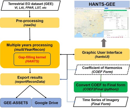
There are three main processing steps in HANTS-GEE (Figure 1):

1. Preprocessing: a gap-filling processing-ready image collection is constructed according to the user-defined EO-based product, spatial and temporal extent. Each image inside the result image collection must contain a ‘dependentBand’ band for the raw data to be gap-filled. The solution of the HANTS method is an iterative linear regression problem, where raw observations are dependent (or response) variables and harmonics are independent (or predictor) variables. Raw datasets need to be rescaled to meaningful ranges and converted to float or double precision type in this step. For example, the raw NDVI products of MODIS sensors, officially released in signed integer type with a scale of 0.0001, are rescaled to a range between −0.2 and 1.0. Users can add new datasets for gap-filling with very little coding work in the ‘rawDs’ function. Currently, supported datasets ready for reconstruction processing are listed in Table 1.

2. Multiple years processing: Current system was mainly designed for remote sensing products from sensors onboard satellites with sun-synchronous orbits, the temporal resolution of which can range from daily to monthly. Although users may request reconstruction tasks spanning one year or several years (e.g. 2001∼2020), the gap-filling is conducted on a yearly basis over the prepared raw dataset in step 1) by calling the ‘hants’ function (i.e. the gap-filling kernel). Unlike the SG filter, HANTS used a global optimal fitting method which pursues the least fitting error for all input observations, and thus if the method is applied to multiple years (e.g. ten years) directly, one can expect the smallest overall fitting error but substantial occasional biases (Zhou et al. 2021). To reconstruct input time series on a yearly basis can effectively reduce local biases. A three-month temporal overlap in default is used for yearly gap-filling to ensure the continuity of processing between consecutive years. For example, to process the NDVI of 2009, raw NDVI observations between October 1, 2008 and March 1, 2010 are used as input to reconstruct the time series between January 1, 2009 and December 31, 2009. The output interval parameter can be set to output results at different temporal resolutions from daily to monthly.

3. Export results: the reconstructed result (image collections) can be exported to either Google Drive or Assets of GEE. In this step, the spatial/temporal resolutions of the output image should be set. Users can export results in four formats, i.e. FINAL, FINAL_RAW, COEF, and COEF-FULL format:

• a) ‘FINAL’ format: reconstructed images with user-specific temporal intervals (e.g. 8-day) over the selected time periods can be exported in Google Drive or Assets. Additionally, a scale and offset parameter can be further set to rescale and convert the final output into 16-bit integer type, which further reduces the data transmission volume (See section 3.2). In this format, all the raw values (where high quality or outliers) are replaced by values extracted from fitted harmonic models. This is the default format for regular long-term time series reconstruction tasks.

• b) ‘FINAL_RAW’ format: the output of this format is very similar to that of ‘FINAL’ format except that only outliers in a time series (identified in step 2 of the model fitting process, see section 2.1) are replaced by values extracted from the well-fitted harmonic model but other high-quality raw data are used as output directly. In this case, for pixels with marginal contaminated observations, the smoothing effect of harmonic fitting can be suppressed compared with the output of ‘FINAL’ format.

• c) ‘COEF’ format: images of harmonic coefficients i.e. coefficients of sine ($b_i$ in Equation (1)) and cosine ($a_i$ in Equation (1)) for each harmonic component, which needs to be converted to time series images (FINAL format) of relevant products by users at local workstations using supplemented python code ((i.e. ‘COEF2Final.py’). It should be mentioned that it is only allowed to extract the coefficients from yearly observations instead of multiple years. For each year, there will be 2*nHarms + 3 coefficient bands in the exported image. The 'COEF’ format was mainly designed to speed up the exporting process and reduce the data transmission (or downloading) volume for users, especially for large-area processing (see section 3.2).

• d) ‘COEF-FULL’ format: The HANTS algorithm can be applied to full input time series (i.e. multiple years) and the amplitude ($A_i$ in Equation (3)) and phase (${\phi }_i$ in Equation (3)) images of each harmonic are exported. The ‘COEF-FULL’ model can capture the general dynamic pattern of pixels (Zhu et al. 2015) and export amplitudes and phases of vegetation time series, which hold valuable phenological information (Menenti et al. 1993, 2010).

Figure 1. Full processing steps of HANTS implementation on GEE. The light-yellow blocks are core steps (functions) implemented on GEE (JavaScript code). The processing of the green block is implemented in Python.

Result data exported to Google Drive can be downloaded by users for further analysis. Results exported to Asserts can be further retrieved into the GEE coding environment through ‘retriveReconColFromAsset’ function and used for other applications in the GEE.

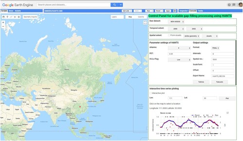
A GUI (Figure 2) was implemented to support users to set all parameters as mentioned earlier, including raw datasets, spatial/temporal extent, HANTS parameters, export settings, etc., without any coding work. The temporal extent setting is determined by all available images of raw datasets, and users can set the temporal processing range by choosing the start year and the end year. The spatial extent can be set by using vector data in Assets or interactively created geometry layers in the map window. Moreover, an interactive plotting function on the GUI can be used to interactively check the reconstruction performance of HANTS for any place on the planet, where both raw and reconstructed time series were plotted in one chart. The software package is available at https://github.com/jiezhou87/HANTS–GEE (accessible on January 30, 2023).

Figure 2. GUI for the scalable gap-filling processing with HANTS.

3. Performance evaluation of HANTS-GEE

3.1. Overall reconstruction accuracy of remote sensing products

3.1.1. The application of HANTS-GEE for different remote sensing products

The HANTS has been documented for reconstructing different remote sensing products such as NDVI, LAI, LST, etc (Julien, Sobrino, and Verhoef 2006; Menenti et al. 2010; de Jong et al. 2011; Alfieri, De Lorenzi, and Menenti 2013; Jiang et al. 2017). And the HANTS-GEE was designed for multiple-source products (as listed in Table 1) processing and the list can be easily expanded by users. Here we intended to provide a general perspective on the capability of the HANTS-GEE to eliminate impacts of problematic observations in EO products by visually checking the reconstruction performance for different products over four selected sites (Table 2). The four selected sites represent different ecosystems and distinct climate conditions (i.e. cloud patterns), which can highlight the adaptability of HANTS-GEE for global reconstruction. Note that all data used in this subsection were extracted from the data products list in Table 1.

Table 2. List, localization and biome sampled by the selected field sites.

Site name	Country	Lat	Lon	Biome
Krasnoyarsk	Russia	57.270	91.600	Needleleaf Forest
Mongu	Zambia	−15.438	23.253	Shrubland/Woodland
Mead	USA	41.165	−96.469	Agriculture (corn/soy)
COMPLET 141	Myanmar	23.452	95.762	Wood Savannas

The HANTS-GEE perfectly recovered a smooth growth curve for each site based on 8-day NDVI observation from MODIS (combined both Terra and Aqua), although less than 50 percent of observations of all sites (except the Mead) were flagged as high quality (QA = 0) (Figure 3A-D). For many cases, even NDVI observations flagged as contaminated by partial cloud (QA = 1), snow (QA = 2), or complete cloud (QA  = 3), these observations did not deviate significantly from the upper envelope of NDVI profiles. This means the QA information provided with vegetation index products may give an inaccurate indication. In other words, contaminated observations flagged by QA should not be excluded directly for time series reconstruction (Zhou et al. 2021). For example, if only high-quality observations (QA = 0) were used in time series reconstruction, continuous gaps lasting more than three months e.g. over Krasnoyarsk, COMPLETE 141, and Mongu may result in failed upper envelop reconstruction. The MODIS LAI profiles have much denser MODIS NDVI profiles (i.e. 4-day vs 8-day) and much more observations are flagged as high quality (i.e. QA = 0) (Figure 3E-H). The HANTS-GEE still can construct a smooth upper envelope of the LAI profile of each selected site very well.

Figure 3. Reconstruction performance of HANTS-GEE for MODIS-NDVI (A-D), MODIS-LAI (E-H), Landsat-NDVI (I-L), and Sentinel-2-NDVI (M-P) products over four sites: Krasnoyarsk, Mongu, Mead, and COMPLETE 141. Raw observations (‘Raw’) and reconstruction result series (‘Recon’) are given in red and blue respectively. Black dots represent quality assessment (QA) value for observation (MODIS-NDVI: 0- Good Data, 1- Marginal Data, 2- Snow/Ice, 3- Cloudy. MODIS-LAI: 0- Good quality (main algorithm with or without saturation), 1- Other quality (back-up algorithm or fill values).).

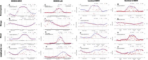
Although the NDVI time series derived from Landsat series satellites (L5, L7, and L8) shared similar temporal resolution (i.e. around 8 days per sample) as the combined NDVI products of MODIS onboard TERRA/AQUA, the latter NDVI time series produced from daily observation using Maximum Value Composition (MVC) hold much denser high-quality observations (Figure 3A-D and Figure 3I-L). In the winter season (from October to March of the following year) of the Krasnoyarsk site (Figure 3I), the long gaps in the NDVI profile from Landsat caused by the dark winter at high latitude resulted in artifacts at the two ends of the reconstructed series. To further address this large gap problem, the pre-filling process suggested by Beck et al. (2006) can be implemented before the HANTS reconstruction. Nevertheless, the smooth growth pattern represented by Landsat observations can be well recovered by HANTS-GEE for each selected site. It should be noted that only one active sensor onboard Landsat-5 was available during 1984∼1999, while the observation density increased gradually after 1999 with the successful launching of Landsat-7/8/9. In this case, the accuracy of the reconstruction result provided by HANTS-GEE might change in different periods. When the HANTS-GEE was applied to process NDVI time series derived from Multispectral Instrument (MSI) sensors onboard Sentinel-2A/B, much more detail can be captured compared to NDVI from Landsat satellites as Sentinel-2/MSI provides a higher revisit frequency (around 4 days) on average (Figure 3M-P).

3.1.2. Case for regional reconstruction effects

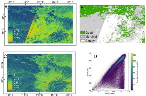
To further demonstrate the effect of time series reconstruction on a regional NDVI image, HANTS-GEE was applied to reconstruct time series of MODIS NDVI (MOD13Q1) images in 2021 of the middle reach of the Yangtze river. The growing season in this region starts in March. The NDVI image on May 9, 2021 (i.e. raw NDVI, Figure 4A) shows rather low values (<0.4) in the central part where only cloudy composited pixels were available in the 16-day MVC processing window (Figure 4B). In addition, the difference in observation quality caused significant ‘edge effect’ in the raw NDVI image (i.e. the edge indicated by the red ellipse in Figure 4A), which is an unrealistic spatial pattern in an NDVI image. The reconstruction processing successfully eliminated the cloud contamination as well as the ‘edge effect’ in the raw NDVI image, where we observed a significant increase of NDVI in the reconstructed image (Figure 4D), especially over the cloud-covered forest area (Figure 4C). The reconstructed NDVI image also presented more reasonable vegetation pattern, with the NDVI of forest area being much higher than that of cropland area.

Figure 4. Reconstructed NDVI image and raw NDVI image of the middle reach of Yangtze river in China: (A) Raw MODIS NDVI (MOD13Q1) on May 9, 2021; (B) Quality control flag for the raw NDVI image; (C) Reconstructed NDVI image by HANTS-GEE; (D) the scatterplot between reconstructed NDVI and raw NDVI images. The ‘red ellipse’ in (A) indicated the sudden change in NDVI (edge effect) caused by a difference in observation quality.

3.1.3. Consistency between HANTS-GEE and HANTS-Python

As mentioned in Section 1, the global reconstruction performance of HANTS had been systematically evaluated by Zhou, Jia, and Menenti (2015) and Zhou et al. (2016a). We prefer the new implementation of HANTS on GEE can completely consistent with the PC-based implementation, in which case the global reconstruction accuracy can be assessed according to our previous performance evaluation result directly. However, the GEE shared a different computation framework compared to local workstations or personal computers, which resulted in a small difference in time series fitting results as mentioned by Kennedy et al. (2018). To evaluate the consistency between the HANTS-GEE and traditional PC-based implementation, we compared the reconstruction result of the MODIS NDVI time series in 2021 using HANTS-GEE and a publicly available implementation of HANTS by Python (see Espinoza-Dávalos et al. 2017, hereafter HANTS-Python). The MODIS NDVI time series in 2021 across BELMANIP2 (BEnchmark Land Multisite ANalysis and Intercomparison of Products) sites were reconstructed by HANTS-GEE and HANTS-Python, respectively. The BELMANIP2 was designed to represent terrestrial vegetation types and their phenology with a set of selected sites, where the percentage of sites for each biome closely matches the global fractional abundance of each biome (Baret et al. 2006). Numerous previous product comparison and performance evaluation studies frequently used BELMANIP2 sites as a reference for global vegetation dynamic patterns (Zhou et al. 2016a; Franch et al. 2017; Zhou et al. 2021). There were 445 sites in the BELMANIP2 dataset, of which 80 non-vegetated sites were excluded from analyses. The parameter setting of HANTS was adopted from Zhou, Jia, and Menenti (2015). The correlation coefficient and root mean squared error (RMSE) between the reconstructed result for each site were calculated to assess the fidelity of implementations.

Among the 365 vegetation-covered sites, more than 310 sites reported very high correlation (>0.99) and low RMSE (<0.02) (Figure 5, Table 3), which indicated rather good consistency between HANTS-GEE and HANTS-Python across most global sites. Across all biomes, the average correlation is larger than 0.92, and the average RMSE is smaller than 0.05. In fact, less-than-ideal consistency mainly appeared at part sites over Evergreen broadleaf forest (EBF) and Evergreen needleleaf forest (ENF) sites. The EBF sites are mainly distributed across tropical rainforest areas where very few clear-sky satellite NDVI observations are available because of frequent cloud coverage (Beck et al. 2006; Julien and Sobrino 2018). In addition, HANTS algorithm aimed to use multiple sinusoidal wave to seasonal dynamic of input signals while the seasonal dynamic of NDVI over EBF sites was rather weak compared to other biomes (Menenti et al. 1993). The limited valid observations and weak seasonal dynamics introduced unstable model fitting and poorer reconstruction performance of HANTS (Zhou, Jia, and Menenti 2015, 2021). The ENF sites are mainly distributed over the Northern high latitude area (around 60°N), where the vegetation may regularly be covered by snow in winter. The snow falling in winter and melting in the next spring normally occurred very fast, which resulted in sudden changes in observed NDVI signals (Beck et al. 2006). The selected low-frequency harmonics of HANTS were not enough to capture such sudden change patterns and caused unstable model fitting in the ENF area as well (Zhou, Jia, and Menenti 2015, 2016a).

Figure 5. Map of the correlation coefficient (A) and Root Mean Squared Error (RMSE) (B) between MODIS NDVI in 2021 reconstructed by HANTS-GEE and HANTS-Python over global BELMANIP2 (BEnchmark Land Multisite ANalysis and Intercomparison of Products) sites. The inset plot inside each map plot is the histogram for corresponding measurement. Sites with maximum yearly NDVI less than 0.2 (i.e. sparse vegetation or bare ground) were excluded. NDVI products from MODIS sensors onboard both Terra and Aqua were used as input for reconstruction.

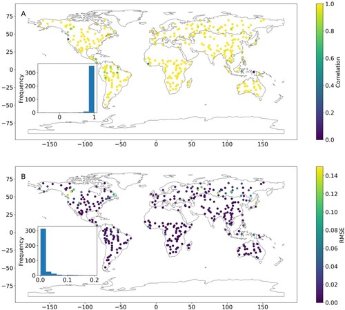
Table 3. Biome-based comparison statistics between HANTS-GEE and HANTS-Python and modified HANTS-Python (HANTS-Python_M). HANTS_Python was provided by Espinoza-Dávalos et al. (2017). HANTS-Python_M was modified from HANTS-Python by adapting the outlier removing procedure as removing all observations with fitting errors larger than FET during each iteration, which is the same procedure applied by HANTS-GEE.

Biomes	HANTS-GEE vs HANTS-PYTHON		HANTS-GEE vs HANTS-PYTHON_M		No. of Sites
	Correlation	RMSE	Correlation	RMSE
Grasses/cereal crops (GCC)	0.998	0.007	0.999	0.005	97
Shrubs (SHR)	0.999	0.005	0.999	0.004	60
Broadleaf crops (BCR)	0.995	0.008	0.999	0.006	19
Savanna (SAV)	0.997	0.008	0.998	0.005	62
Evergreen broadleaf forest (EBF)	0.922	0.012	0.992	0.004	61
Deciduous broadleaf forest (DBF)	0.990	0.020	0.998	0.012	28
Evergreen needleleaf forest (ENF)	0.942	0.041	0.972	0.026	29
Deciduous needle-leaf forest (DNF)	0.984	0.037	0.992	0.030	9
Average	0.978	0.017	0.994	0.012	-

As regards the slight discrepancy between the HANTS-GEE and HANTS-Python, there were at least two factors that should be mentioned. Firstly, in the HANTS-Python implemented by Espinoza-Dávalos et al. (2017), only the observation with the largest fitting error (and larger than the FET at the same time) is removed as outliers during each iteration (i.e. one outlier each iteration). However, the HANTS-GEE removed all observations with fitting errors larger than FET as outliers during each iteration (i.e. all outliers each iteration). To check the effect of this difference on the consistency, the original HANTS-Python was modified to ‘all outlier each iteration’ (i.e. HANTS-Python_M). Compared with the original HANTS-Python, the consistency between HANTS-GEE and HANTS-Python_M was further improved significantly in terms of both correlation and RMSE (Table 3). Particularly, the correlation increased from 0.0.922 (0.939) to 0.992 (0.972) and RMSE decreased from 0.012 (0.041) to 0.004 (0.026) over the EBF (ENF) sites. Until now no conclusion on which outlier removing strategies performs better for global reconstruction. In fact, even with different outlier removing strategies the consistency across biomes is rather high (see the ‘HANTS-GEE vs HANTS-Python’ column of Table 3). In addition, the implementation of the ‘one outlier each iteration’ procedure is rather complex in GEE currently. In this case, we kept the ‘all outlier one iteration’ strategy in HANTS-GEE. Secondly, both two implementations used ridge regression to solve the constructed harmonic models, however, the GEE and python respectively applied the Cholesky decomposition method and lower – upper (LU) decomposition method in backends to solve linear systems. This can explain the remaining small difference between HANTS-GEE and HANTS-Python_M even with the same procedures (see the ‘HANTS-GEE vs HANTS-PYTHON_M’ column of Table 3).

3.2. Processing efficiency

One main purpose of HANTS-GEE is to provide efficient time series reconstruction services for users by taking advantage of the powerful computing resource of the GEE platform. Users may submit a reconstruction task for products with large spatial extent (e.g. global), long time periods (e.g. 10 years), or high spatial resolution (e.g. 10 m for Sentinel-2), where processing speed becomes the core concern of users. However, the final computing speed of a specific reconstruction task is dependent on the computing resource (e.g. the number of CPUs) allocated by the data management system of GEE in real-time by accounting for the total resource available in the resource pools (Gorelick et al. 2017; Tamiminia et al. 2020). In this case, the same task submitted at a different time may take a very different processing time. Taking a reconstruction task for one year global 5-km 16-day NDVI product of MODIS as an example, the processing time with HANTS-GEE can range from 15 min to 50 min. As a comparison, the processing time on a local workstation with 8-processing cores for the same task is 106 min, whereas the HANTS was parallelly implemented with Python.

Time series reconstruction in remote sensing is a data and computation-intensive process. The reconstruction results of HANTS-GEE were exported either to Google Drive or the GEE Asserts, which hold quota restrictions for google users (e.g. 15 Gigabyte free storage for Google Drive). The reconstruction tasks cannot succeed without upgrading the storage space for exported file volumes exceeding the upper limits. On the other hand, users usually need to download exported reconstruction results in Google drive to local workstations for further analysis. The limited internet bandwidths in some world regions may become the main bottleneck for further applications. To reduce the data transmission volume, users of HANTS-GEE can choose to export coefficients of harmonic components (i.e. ai and bi in Equation (1)) instead of the final reconstructed image time series by setting exporting format as ‘COEF’. In this case, the number of bands of exported GeoTIFF image ( =  2*NF + 1) will be no more than 13 as the NF for vegetation index reconstruction is normally set smaller than 6 (Zhou et al. 2021). Practically, to produce an 8-day gap-free NDVI product in ‘FINAL’ format, there will be 46 images to be exported. In general, if 4 harmonics are used in HANTS, there will be 9 coefficients in total for an annual reconstruction thus there will be 9 images to be exported in ‘COEF’ format, which results in an 80% reduction in data transmission volume compared to the ‘FINAL’ format. Even if 6 harmonic components were used, there would still be a 71% data volume reduction. In addition, the data type of exported images in ‘FINAL’ format is converted from double float (64-bit) to signed integer (16-bit) by the scale and offset settings, which further reduced data transmission volume.

4. Discussion

Time series reconstruction is a critical data processing step for most remote sensing applications, especially for observations or products acquired by optical or thermal sensors (Holben 1986; Zhou, Jia, and Menenti 2015; Yu et al. 2022b). A panoply of TSR algorithms has been proposed in the past decades, and various studies on different regions had extensively evaluated their performances. However, the lack of convenient and efficient software packages or tools specified for TSR purposes hampered the popularity of these TSR algorithms for non-professional users or non-academic communities. The proposed HANTS-GEE provided users with a scalable tool for rapid and efficient time series reconstruction of remote sensing products. The scalability is mainly achieved by offering users customizable TSR services across both temporal and spatial scales, as well as by the full temporal and spatial coverage where raw remote sensing observation or products are available on GEE. Powered by the GEE, the HANTS-GEE improved traditional workstation-based time series processing of remote sensing products by 1) transferring complex data processing procedures such as image mosaic, resampling, and reprojection to the GEE server; 2) speeding up the processing by paralleling based on the scalable computation and storage resources of GEE; 3) reducing the data transmission volume more than 50% by the data compression capability of HANTS. Moreover, the implementation of the kernel algorithm (i.e. ‘hants’ function) completely follows the procedures described by Roerink, Menenti, and Verhoef (2000) and Zhou, Jia, and Menenti (2015). The suitability of using HANTS-GEE for multiple product reconstruction was illustrated by reconstructing time series of different remote sensing products over four representative sites and a regional reconstruction case. Our analysis further proved that the HANTS-GEE can provide users with consistent reconstruction results with that of PC-based HANTS implementation (HANTS-Python) over the most terrestrial vegetated surface. In other words, the HANTS-GEE shared a similar reconstruction performance with HANTS-Python. In this case, users can refer to Zhou, Jia, and Menenti (2015) and Zhou et al. (2016a) for quantified global reconstruction accuracy of HANTS. Except for the datasets listed in Table 1, users can ingest other datasets derived from the remote sensing dataset on GEE by a limited revision to the ‘rawDs’ function. Users can also upload their datasets to the GEE assets and ingest them to HANTS-GEE for high-efficiency reconstruction.

The frequency-based methods such as Fourier analysis (Menenti et al. 1993), harmonic analysis (Jakubauskas, Legates, and Kastens 2002), and generalized spectral analysis (Malamiri et al. 2018) have popularized in time series analysis of remote sensed data. It should be mentioned that the current implementation of HANTS-GEE strictly followed procedures of the HANTS algorithm proposed by Verhoef, Menenti, and Azzali (1996) and Roerink, Menenti, and Verhoef (2000). In a narrow sense, the HANTS was aimed to reconstruct remote sensed time series with biased observations by constructing harmonic models and removing outliers iteratively. The HANTS should be differentiated from general harmonic analysis methods that are directly applied to gapped time series in that outliers had been identified with ancillary information and removed in advance. The latter pays more attention to filling existing gaps and extracting the seasonality of time series (e.g. Jakubauskas, Legates, and Kastens 2002; Zhu and Woodcock 2014). We already noted several studies argued that they implemented HANTS on GEE by referring to the script shared by Nick Clinton at https://goo.gl/lMwd2Y (Xie and Fan 2021; Yang et al. 2022a, 2022b). It seems these studies only used harmonic models to fit time series but didn’t iteratively remove outliers, which is a kind of misuse of HANTS. The classic HANTS has been implemented with different programming languages and gets widely used in the remote sensing community (Zhou et al. 2021). The advantage and drawbacks of the classic algorithm were thoroughly discussed and understood by users through previous applications and performance evaluation works (e.g. Zhou, Jia, and Menenti 2015; Hermance 2007). One can expect more and more users may apply the classic HANTS algorithm for time series reconstruction in remote sensing. In this context, we believe the implementation of such a classic HANTS algorithm in GEE will provide a great convenience for potential users.

Based on the current implementation of classical HANTS on GEE, several potential improvements can be expected in the future. Hermance (2007) introduceed a penalty function of roughness damper to the OLS solver of harmonic models for stable fitting with high-order harmonics. Zhou et al. (2022) proposed the Harmonic Adaptive Penalty Operator (HAPO) for harmonic analysis of unevenly distributed time series. By introducing a new penalty function to minimize unexpected fluctuations in the model, the overfitting issue of regression in time series with temporal gaps was substantially reduced. These strategies can promote the robustness of the solution for constructed linear harmonic models. In addition, Zhou et al. (2021) optimize the parameters of HANTS for global NDVI reconstruction and proposed suggestions for biome – specific parameter settings, which can be further introduced in the HANTS-GEE tool for automatic parameter setting.

In general, the HANTS-GEE provided a cloud-based framework for full-stack TSR purposes. The tool can be further improved in several aspects in the future. Firstly, more TSR algorithms can be further embedded in the framework to fulfill accuracy requirements for different regions as the performance of TSR algorithms always presented significant spatial heterogeneity (Zhou et al. 2016a; Julien and Sobrino 2018). The SG and WS algorithms had been implemented on GEE (Kong et al. 2019; Chen et al. 2021) and can be easily adapted to the current framework. At the same time, it should be noted that not all TSR can be easily implemented with the restricted API provided by GEE, especially for algorithms relying on non-linear systems such as DL and AG (Jönsson and Eklundh 2004; Zhou et al. 2016a). Secondly, some intermediate time series feature extraction procedures, such as phenology metrics extraction and vegetation anomaly detection, can be further implemented in the tool, which can facilitate users interested in general time series analysis of remote sensing products on GEE. Moreover, the GUI of HANTS-GEE was implemented with the limited user interface API provided by GEE, which can be further improved by designing a new browser-based GUI for HANTS-GEE via the python API of GEE.

Nevertheless, algorithms for time-series reconstruction such as HANTS, relying only on temporal high-quality observations for model fitting, ensured the independence of ancillary information and the capacity to be adapted to reconstruct any time series of remotely sensed data. However, raw time series with insufficient high-quality observations (e.g. temporally continuous cloud coverage or low revisiting frequency) may challenge these TSR methods. For example, although the current HANTS-GEE can be used to reconstruct the NDVI time series of Landsat since 1984 practically, the reconstruction performance for some regions can be quite questionable, especially before 2000, due to unbalanced regional satellite data receiving capability (Wulder et al. 2016). Advanced solutions such as combining spatiotemporal information together (Chu et al. 2021; Yan and Roy 2020), and fusing observations from multiple sensors (Gao et al. 2006; Qiu et al. 2021) have been proposed for better reconstruction performance. Further efforts should be dedicated to embedding these strategies into HANTS-GEE to mitigate the reconstruction challenges for cloud-prone and observation-inadequate areas.

5. Conclusion

Time series reconstruction is an important pre-processing procedure for most applications based on long time-series remote sensing products. In practice, the procedure is data and computation intensive no matter which methods users applied. In this case, the processing efficiency should also be considered in addition to reconstruction accuracy to provide better time series reconstruction service for users. This paper introduced an implementation of the well-evaluated and widely applied Harmonic ANalysis of Time Series (HANTS) on the cloud-based GEE platform (i.e. HANTS-GEE) for scalable time series reconstructing of terrestrial remotely sensed products. The performance evaluation result suggested that the HANTS-GEE can achieve comparable reconstruction accuracy as the workstation-based HANTS implemented with Python while providing appreciable improvement in processing efficiency via the powerful computation and storage capacity of the GEE. The code and detailed user manual can be found at https://github.com/jiezhou87/HANTS–GEE where any bugs and issues related to the tool can be reported by users. Further work on improving reconstruction accuracy, enriching time series processing functions, as well adapting the graphic user interface of the tool can be expected in future.

Disclosure statement

No potential conflict of interest was reported by the author(s).

Data availability statement

The code and user manual of HANTS-GEE were shared via GitHub repository: https://github.com/jiezhou87/HANTS–GEE.

Additional information

Funding

The study was financially supported by the National Natural Science Foundation of China (grant number 42171371 and No. 41701492). Massimo Menenti acknowledges the support of the MOST High-Level Foreign Expert program (grant number G2022055010L) and the Chinese Academy of Sciences President's International Fellowship Initiative (grant number 2020VTA0001).

References

- Alfieri, S. M., F. De Lorenzi, and M. Menenti. 2013. “Mapping Air Temperature Using Time Series Analysis of LST: The SINTESI Approach.” Nonlin. Processes Geophys 20 (4): 513–527. doi:10.5194/npg-20-513-2013.
- Arévalo, Paulo, Eric L Bullock, Curtis E Woodcock, and Pontus Olofsson. 2020. “A Suite of Tools for Continuous Land Change Monitoring in Google Earth Engine.” Frontiers in Climate 2: 26. doi:10.3389/fclim.2020.576740
- Baret, F., J. T. Morissette, R. A. Fernandes, J. L. Champeaux, R. B. Myneni, J. Chen, S. Plummer, et al. 2006. “Evaluation of the Representativeness of Networks of Sites for the Global Validation and Intercomparison of Land Biophysical Products: Proposition of the CEOS-BELMANIP.” IEEE Transactions on Geoscience and Remote Sensing 44 (July): 1794–1803. doi:10.1109/TGRS.2006.876030
- Beck, Pieter S. A., Clement Atzberger, Kjell Arild Høgda, Bernt Johansen, and Andrew K. Skidmore. 2006. “Improved Monitoring of Vegetation Dynamics at Very High Latitudes: A New Method Using MODIS NDVI.” Remote Sensing of Environment 100 (3): Elsevier: 321–334. doi:10.1016/j.rse.2005.10.021
- Belda, Santiago, Luca Pipia, Pablo Morcillo-Pallarés, Juan Pablo Rivera-Caicedo, Eatidal Amin, Charlotte De Grave, and Jochem Verrelst. 2020. “DATimeS: A Machine Learning Time Series GUI Toolbox for Gap-Filling and Vegetation Phenology Trends Detection.” Environmental Modelling & Software 127: 104666. doi:10.1016/j.envsoft.2020.104666
- Bretherton, Francis P. 1985. “Earth System Science and Remote Sensing.” Proceedings of the IEEE 73 (6): 1118–1127. doi:10.1109/PROC.1985.13242
- Cao, Ruyin, Yang Chen, Miaogen Shen, Jin Chen, Ji Zhou, Cong Wang, and Wei Yang. 2018. “A Simple Method to Improve the Quality of NDVI Time-Series Data by Integrating Spatiotemporal Information with the Savitzky-Golay Filter.” Remote Sensing of Environment 217: Elsevier: 244–257. doi:10.1016/j.rse.2018.08.022
- Chen, Yang, Ruyin Cao, Jin Chen, Licong Liu, and Bunkei Matsushita. 2021. “A Practical Approach to Reconstruct High-Quality Landsat NDVI Time-Series Data by Gap Filling and the Savitzky–Golay Filter.” ISPRS Journal of Photogrammetry and Remote Sensing 180: 174–190. doi:10.1016/j.isprsjprs.2021.08.015
- Chen, Jin, Per Jönsson, Masayuki Tamura, Zhihui Gu, Bunkei Matsushita, and Lars Eklundh. 2004. “A Simple Method for Reconstructing a High-Quality NDVI Time-Series Data Set Based on the Savitzky–Golay Filter.” Remote Sensing of Environment 91 (3–4): Elsevier: 332–344. doi:10.1016/j.rse.2004.03.014
- Chu, Dong, Huanfeng Shen, Xiaobin Guan, Jing M Chen, Xinghua Li, Jie Li, and Liangpei Zhang. 2021. “Long Time-Series NDVI Reconstruction in Cloud-Prone Regions via Spatio-Temporal Tensor Completion.” Remote Sensing of Environment 264: 112632. doi:10.1016/j.rse.2021.112632
- de Jong, Rogier, Sytze de Bruin, Allard de Wit, Michael E. Schaepman, and David L. Dent. 2011. “Analysis of Monotonic Greening and Browning Trends from Global NDVI Time-Series.” Remote Sensing of Environment 115: 692–702. doi:10.1016/j.rse.2010.10.011.
- Eerens, Herman, Dominique Haesen, Felix Rembold, Ferdinando Urbano, Carolien Tote, and Lieven Bydekerke. 2014. “Image Time Series Processing for Agriculture Monitoring.” Environmental Modelling & Software 53: 154–162. doi:10.1016/j.envsoft.2013.10.021
- Eklundh, L., and P. Jönsson. 2012. “TIMESAT 3.1 Software Manual.” Lund University, Sweden, 1–82.
- Eklundh, L., and P. Jönsson. 2017. “TIMESAT 3.3 with Seasonal Trend Decomposition and Parallel Processing Software Manual.” Lund, Sweden: Lund University.
- Espinoza-Dávalos, G. E., W. G. M. Bastiaanssen, B. Bett, and X. Cai. 2017. “A Python Implementation of the Harmonic ANalysis of Time Series (HANTS) Algorithm for Geospatial Data”. doi:10.5281/zenodo.820623.
- Fang, Hongliang, Shunlin Liang, John R. Townshend, and Robert E. Dickinson. 2008. “Spatially and Temporally Continuous LAI Data Sets Based on an Integrated Filtering Method: Examples from North America.” Remote Sensing of Environment 112 (1): Elsevier: 75–93. doi:10.1016/j.rse.2006.07.026
- Franch, Belen, Eric Vermote, Jean-Claude Roger, Emilie Murphy, Inbal Becker-Reshef, Chris Justice, Martin Claverie, et al. 2017. “A 30+ Year AVHRR Land Surface Reflectance Climate Data Record and Its Application to Wheat Yield Monitoring.” Remote Sensing 9 (3): 296. doi:10.3390/rs9030296.
- Gao, Feng, Jeff Masek, Matt Schwaller, and Forrest Hall. 2006. “On the Blending of the Landsat and MODIS Surface Reflectance: Predicting Daily Landsat Surface Reflectance.” IEEE Transactions on Geoscience and Remote Sensing 44 (8): 2207–2218. doi:10.1109/TGRS.2006.872081
- Geng, Liying, Mingguo Ma, Xufeng Wang, Wenping Yu, Shuzhen Jia, and Haibo Wang. 2014. “Comparison of Eight Techniques for Reconstructing Multi-Satellite Sensor Time-Series NDVI Data Sets in the Heihe River Basin, China.” Remote Sensing 6 (3): MDPI: 2024–2049. doi:10.3390/rs6032024
- Gomes, Vitor CF, Gilberto R Queiroz, and Karine R Ferreira. 2020. “An Overview of Platforms for Big Earth Observation Data Management and Analysis.” Remote Sensing 12 (8): 1253. doi:10.3390/rs12081253
- Gorelick, Noel, Matt Hancher, Mike Dixon, Simon Ilyushchenko, David Thau, and Rebecca Moore. 2017. “Google Earth Engine: Planetary-Scale Geospatial Analysis for Everyone.” Remote Sensing of Environment 202: 18–27. doi:10.1016/j.rse.2017.06.031
- Guo, Huadong, Stefano Nativi, Dong Liang, Max Craglia, Lizhe Wang, Sven Schade, Christina Corban, et al. 2020. “Big Earth Data Science: An Information Framework for a Sustainable Planet.” International Journal of Digital Earth 13 (7): 743–767. doi:10.1080/17538947.2020.1743785
- Guo, Huadong, Lizhe Wang, and Dong Liang. 2016. “Big Earth Data from Space: A New Engine for Earth Science.” Science Bulletin 61 (7): 505–513. doi:10.1007/s11434-016-1041-y
- Hamunyela, Eliakim, Sabina Rosca, Andrei Mirt, Eric Engle, Martin Herold, Fabian Gieseke, and Jan Verbesselt. 2020. “Implementation of BFASTmonitor Algorithm on Google Earth Engine to Support Large-Area and Sub-Annual Change Monitoring Using Earth Observation Data.” Remote Sensing 12 (18): 2953. doi:10.3390/rs12182953
- Hermance, John F. 2007. “Stabilizing High-Order, Non-Classical Harmonic Analysis of NDVI Data for Average Annual Models by Damping Model Roughness.” International Journal of Remote Sensing 28 (12): Taylor & Francis: 2801–2819. doi:10.1080/01431160600967128
- Hird, Jennifer N., and Gregory J. McDermid. 2009. “Noise Reduction of NDVI Time Series: An Empirical Comparison of Selected Techniques.” Remote Sensing of Environment 113 (1): Elsevier: 248–258. doi:10.1016/j.rse.2008.09.003
- Holben, Brent N. 1986. “Characteristics of Maximum-Value Composite Images from Temporal AVHRR Data.” International Journal of Remote Sensing 7 (11): 1417–1434. doi:10.1080/01431168608948945
- Huntington, Justin L., Katherine C. Hegewisch, Britta Daudert, Charles G. Morton, John T. Abatzoglou, Daniel J. McEvoy, and Tyler Erickson. 2017. “Climate Engine: Cloud Computing and Visualization of Climate and Remote Sensing Data for Advanced Natural Resource Monitoring and Process Understanding.” Bulletin of the American Meteorological Society 98 (11): 2397–2410. doi:10.1175/BAMS-D-15-00324.1
- Jakubauskas, Mark E, David R Legates, and Jude H Kastens. 2002. “Crop Identification Using Harmonic Analysis of Time-Series AVHRR NDVI Data.” Computers and Electronics in Agriculture 37 (1–3): Elsevier: 127–139. doi:10.1016/S0168-1699(02)00116-3
- Jia, Li, H. Shang, G. Hu, and M. Menenti. 2011. “Phenological Response of Vegetation to Upstream River Flow in the Heihe Rive Basin by Time Series Analysis of MODIS Data.” Hydrology and Earth System Sciences 15 (3): 1047–1064. doi:10.5194/hess-15-1047-2011
- Jiang, Chongya, Youngryel Ryu, Hongliang Fang, Ranga Myneni, Martin Claverie, and Zaichun Zhu. 2017. “Inconsistencies of Interannual Variability and Trends in Long-Term Satellite Leaf Area Index Products.” Global Change Biology 23 (10): 4133–4146. doi:10.1111/gcb.13787.
- Jonsson, Per, and Lars Eklundh. 2002. “Seasonality Extraction by Function Fitting to Time-Series of Satellite Sensor Data.” IEEE Transactions on Geoscience and Remote Sensing 40 (8): IEEE: 1824–1832. doi:10.1109/TGRS.2002.802519
- Jönsson, Per, and Lars Eklundh. 2004. “TIMESAT—a Program for Analyzing Time-Series of Satellite Sensor Data.” Computers & Geosciences 30 (8): 833–845. doi:10.1016/j.cageo.2004.05.006
- Jönsson, Per, and Lars Eklundh. 2007. “TIMESAT-a Program for Analyzing Time-Series of Satellite Sensor Data. Users Guide for TIMESAT 2.3.” Malmö and Lund.
- Julien, Yves, and Jose Sobrino. 2018. “TISSBERT: A Benchmark for the Validation and Comparison of NDVI Time Series Reconstruction Methods.” Revista de Teledetección 2018 (June): 19–31. doi:10.4995/raet.2018.9749.
- Julien, Yves, and José A. Sobrino. 2019. “Optimizing and Comparing Gap-Filling Techniques Using Simulated NDVI Time Series from Remotely Sensed Global Data.” International Journal of Applied Earth Observation and Geoinformation 76: Elsevier: 93–111. doi:10.1016/j.jag.2018.11.008
- Julien, Yves, José A. Sobrino, and Wout Verhoef. 2006. “Changes in Land Surface Temperatures and NDVI Values Over Europe between 1982 and 1999.” Remote Sensing of Environment 103 (1): 43–55. doi:10.1016/j.rse.2006.03.011.
- Kennedy, Robert E, Zhiqiang Yang, Noel Gorelick, Justin Braaten, Lucas Cavalcante, Warren B Cohen, and Sean Healey. 2018. “Implementation of the LandTrendr Algorithm on Google Earth Engine.” Remote Sensing 10 (5): 691. doi:10.3390/rs10050691
- Kong, Dongdong, Yongqiang Zhang, Xihui Gu, and Dagang Wang. 2019. “A Robust Method for Reconstructing Global MODIS EVI Time Series on the Google Earth Engine.” ISPRS Journal of Photogrammetry and Remote Sensing 155: 13–24. doi:10.1016/j.isprsjprs.2019.06.014
- Li, Huan, Wei Wan, Yu Fang, Siyu Zhu, Xi Chen, Baojian Liu, and Yang Hong. 2019. “A Google Earth Engine-Enabled Software for Efficiently Generating High-Quality User-Ready Landsat Mosaic Images.” Environmental Modelling & Software 112: 16–22. doi:10.1016/j.envsoft.2018.11.004.
- Li, Shuang, Liang Xu, Yinghong Jing, Hang Yin, Xinghua Li, and Xiaobin Guan. 2021. “High-Quality Vegetation Index Product Generation: A Review of NDVI Time Series Reconstruction Techniques.” International Journal of Applied Earth Observation and Geoinformation 105: 102640. doi:10.1016/j.jag.2021.102640
- Lu, Xiaoliang, Ronggao Liu, Jiyuan Liu, and Shunlin Liang. 2007. “Removal of Noise by Wavelet Method to Generate High Quality Temporal Data of Terrestrial MODIS Products.” Photogrammetric Engineering & Remote Sensing 73 (10): American Society for Photogrammetry and Remote Sensing: 1129–1139. doi:10.14358/PERS.73.10.1129
- Malamiri, Ghafarian, Hamid Reza, Iman Rousta, Haraldur Olafsson, Hadi Zare, and Hao Zhang. 2018. “Gap-Filling of MODIS Time Series Land Surface Temperature (LST) Products Using Singular Spectrum Analysis (SSA).” Atmosphere 9 (9): MDPI: 334. doi:10.3390/atmos9090334
- Menenti, M., S. Azzali, W. Verhoef, and R. Van Swol. 1991. Mapping Agroecological Zones and Timelag in Vegetation by Means of Fourier Analysis of Time Scenes of NDVl Images. Report 32. Monitoring Agroecological Resources with Remote Sensing & Simulation. Wageningen (The Netherlands): DLO The Winand Staring Centre, R. Https://edepot.wur.nl/360548.
- Menenti, M., S. Azzali, W. Verhoef, and R. Van Swol. 1993. “Mapping Agroecological Zones and Time Lag in Vegetation Growth by Means of Fourier Analysis of Time Series of NDVI Images.” Advances in Space Research 13 (5): 233–237. doi:10.1016/0273-1177(93)90550-U
- Menenti, Massimo, Li Jia, S. Azzali, G. Roerink, María Loyarte, and Saturnino Leguizamón. 2010. “Analysis of Vegetation Response to Climate Variability Using Extended Time Series of Multispectral Satellite Images.” In Remote Sensing Optical Observation of Vegetation Properties, edited by Fabio Maselli, Massimo Menenti, and Pietro Alessandro Brivio, 131–163. Kerala, India: Research Signpost.
- Padhee, Suman Kumar, and Subashisa Dutta. 2019. “Spatio-Temporal Reconstruction of MODIS NDVI by Regional Land Surface Phenology and Harmonic Analysis of Time-Series.” GIScience & Remote Sensing 56 (8): Taylor & Francis: 1261–1288. doi:10.1080/15481603.2019.1646977
- Potgieter, A. B., A. Apan, P. Dunn, and G. Hammer. 2007. “Estimating Crop Area Using Seasonal Time Series of Enhanced Vegetation Index from MODIS Satellite Imagery.” Australian Journal of Agricultural Research 58 (4): 316. doi:10.1071/AR06279
- Qiu, Yuean, Junxiong Zhou, Jin Chen, and Xuehong Chen. 2021. “Spatiotemporal Fusion Method to Simultaneously Generate Full-Length Normalized Difference Vegetation Index Time Series (SSFIT).” International Journal of Applied Earth Observation and Geoinformation 100: 102333. doi:10.1016/j.jag.2021.102333
- Reichstein, M., G. Camps-Valls, B. Stevens, M. Jung, J. Denzler, and N. Carvalhais. 2019. “Deep Learning and Process Understanding for Data-Driven Earth System Science.” Nature 566 (7743): 195–204. doi:10.1038/s41586-019-0912-1
- Rembold, Felix, Michele Meroni, Ferdinando Urbano, Antoine Royer, Clement Atzberger, Guido Lemoine, Herman Eerens, and Dominque Haesen. 2015. “Remote Sensing Time Series Analysis for Crop Monitoring with the SPIRITS Software: New Functionalities and Use Examples.” Frontiers in Environmental Science 3: 46. doi:10.3389/fenvs.2015.00046
- Roerink, G. J., M. Menenti, W. Soepboer, and Zhongbo Su. 2003. “Assessment of Climate Impact on Vegetation Dynamics by Using Remote Sensing.” Physics and Chemistry of the Earth, Parts A/B/C 28 (1–3): 103–109. doi:10.1016/S1474-7065(03)00011-1
- Roerink, G. J., Massimo Menenti, and Wout Verhoef. 2000. “Reconstructing Cloudfree NDVI Composites Using Fourier Analysis of Time Series.” International Journal of Remote Sensing 21 (9): 1911–1917. doi:10.1080/014311600209814
- Shang, Haolu, Li Jia, and Massimo Menenti. 2015. “Analyzing the Inundation Pattern of the Poyang Lake Floodplain by Passive Microwave Data.” Journal of Hydrometeorology 16 (April): 652–667. doi:10.1175/JHM-D-14-0022.1.
- Shen, Huanfeng, Xinghua Li, Qing Cheng, Chao Zeng, Gang Yang, Huifang Li, and Liangpei Zhang. 2015. “Missing Information Reconstruction of Remote Sensing Data: A Technical Review.” IEEE Geoscience and Remote Sensing Magazine 3 (3): 61–85. doi:10.1109/MGRS.2015.2441912.
- Shiklomanov, Alexey N, Bethany A Bradley, Kyla M Dahlin, Andrew M Fox, Christopher M Gough, Forrest M Hoffman, Elizabeth M Middleton, Shawn P Serbin, Luke Smallman, and William K Smith. 2019. “Enhancing Global Change Experiments Through Integration of Remote-Sensing Techniques.” Frontiers in Ecology and the Environment 17 (4): 215–224. doi:10.1002/fee.2031
- Steffen, Will, Katherine Richardson, Johan Rockström, Hans Joachim Schellnhuber, Opha Pauline Dube, Sébastien Dutreuil, Timothy M Lenton, and Jane Lubchenco. 2020. “The Emergence and Evolution of Earth System Science.” Nature Reviews Earth & Environment 1 (1): 54–63. doi:10.1038/s43017-019-0005-6
- Tamiminia, Haifa, Bahram Salehi, Masoud Mahdianpari, Lindi Quackenbush, Sarina Adeli, and Brian Brisco. 2020. “Google Earth Engine for Geo-Big Data Applications: A Meta-Analysis and Systematic Review.” ISPRS Journal of Photogrammetry and Remote Sensing 164: 152–170. doi:10.1016/j.isprsjprs.2020.04.001
- Verbesselt, Jan, Achim Zeileis, and Martin Herold. 2012. “Near Real-Time Disturbance Detection Using Satellite Image Time Series.” Remote Sensing of Environment 123: 98–108. doi:10.1016/j.rse.2012.02.022
- Verhoef, W. 1996. Application of Harmonic Analysis of NDVI Time Series (HANTS). Wageningen, The Netherlands: Fourier Analysis of Temporal NDVI in the Southern African and American Continents. DLO Winand Staring Centre.
- Verhoef, W., M. Menenti, and S. Azzali. 1996. “A Colour Composite of NOAA-AVHRR-NDVI Based on Time Series Analysis (1981-1992).” International Journal of Remote Sensing 17 (January): 231–235. doi:10.1080/01431169608949001
- Wagemann, Julia, Stephan Siemen, Bernhard Seeger, and Jörg Bendix. 2021. “A User Perspective on Future Cloud-Based Services for Big Earth Data.” International Journal of Digital Earth 14 (12): 1758–1774. doi:10.1080/17538947.2021.1982031
- Wulder, Michael A, Joanne C White, Thomas R Loveland, Curtis E Woodcock, Alan S Belward, Warren B Cohen, Eugene A Fosnight, Jerad Shaw, Jeffrey G Masek, and David P Roy. 2016. “The Global Landsat Archive: Status, Consolidation, and Direction.” Remote Sensing of Environment 185: 271–283. doi:10.1016/j.rse.2015.11.032
- Xian, George Z, Kelcy Smith, Danika Wellington, Josephine Horton, Qiang Zhou, Congcong Li, Roger Auch, Jesslyn F Brown, Zhe Zhu, and Ryan R Reker. 2022. “Implementation of the CCDC Algorithm to Produce the LCMAP Collection 1.0 Annual Land Surface Change Product.” Earth System Science Data 14 (1): 143–162. doi:10.5194/essd-14-143-2022
- Xie, Fei, and Hui Fan. 2021. “Deriving Drought Indices from MODIS Vegetation Indices (NDVI/EVI) and Land Surface Temperature (LST): Is Data Reconstruction Necessary?” International Journal of Applied Earth Observation and Geoinformation 101: Elsevier: 102352. doi:10.1016/j.jag.2021.102352
- Yan, Lin, and David P Roy. 2020. “Spatially and Temporally Complete Landsat Reflectance Time Series Modelling: The Fill-and-Fit Approach.” Remote Sensing of Environment 241: 111718. doi:10.1016/j.rse.2020.111718
- Yang, Yingpin, Jiancheng Luo, Qiting Huang, Wei Wu, and Yingwei Sun. 2019. “Weighted Double-Logistic Function Fitting Method for Reconstructing the High-Quality Sentinel-2 NDVI Time Series Data Set.” Remote Sensing 11 (20): MDPI: 2342. doi:10.3390/rs11202342
- Yang, Xinyue, Fei Meng, Pingjie Fu, Yuqiang Wang, and Yaohui Liu. 2022a. “Time-Frequency Optimization of RSEI: A Case Study of Yangtze River Basin.” Ecological Indicators 141: Elsevier: 109080. doi:10.1016/j.ecolind.2022.109080
- Yang, Xinyue, Fei Meng, Pingjie Fu, Jiawei Zhang, and Yaohui Liu. 2022b. “Instability of Remote Sensing Ecological Index and Its Optimisation for Time Frequency and Scale.” Ecological Informatics 72: Elsevier: 101870. doi:10.1016/j.ecoinf.2022.101870
- Yu, Bo, Chong Xu, Fang Chen, Ning Wang, and Lei Wang. 2022a. “HADeenNet: A Hierarchical-Attention Multi-Scale Deconvolution Network for Landslide Detection.” International Journal of Applied Earth Observation and Geoinformation 111: 102853. doi:10.1016/j.jag.2022.102853.
- Yu, Bo, Aqiang Yang, Fang Chen, Ning Wang, and Lei Wang. 2022b. “SNNFD, Spiking Neural Segmentation Network in Frequency Domain Using High Spatial Resolution Images for Building Extraction.” International Journal of Applied Earth Observation and Geoinformation 112: 102930. doi:10.1016/j.jag.2022.102930.
- Zeng, Linglin, Brian D Wardlow, Daxiang Xiang, Shun Hu, and Deren Li. 2020. “A Review of Vegetation Phenological Metrics Extraction Using Time-Series, Multispectral Satellite Data.” Remote Sensing of Environment 237: 111511. doi:10.1016/j.rse.2019.111511
- Zhang, Chen, Liping Di, Zhengwei Yang, Li Lin, and Pengyu Hao. 2020. “AgKit4EE: A Toolkit for Agricultural Land Use Modeling of the Conterminous United States Based on Google Earth Engine.” Environmental Modelling & Software 129: 104694. doi:10.1016/j.envsoft.2020.104694
- Zhang, Junxue, Rong Shang, Chadwick Rittenhouse, Chandi Witharana, and Zhe Zhu. 2021. “Evaluating the Impacts of Models, Data Density and Irregularity on Reconstructing and Forecasting Dense Landsat Time Series.” Science of Remote Sensing 4: 100023. doi:10.1016/j.srs.2021.100023
- Zhao, Feng, Rui Sun, Liheng Zhong, Ran Meng, Chengquan Huang, Xiaoxi Zeng, Mengyu Wang, Yaxin Li, and Ziyang Wang. 2022. “Monthly Mapping of Forest Harvesting Using Dense Time Series Sentinel-1 SAR Imagery and Deep Learning.” Remote Sensing of Environment 269: 112822. doi:10.1016/j.rse.2021.112822
- Zhou, Jie, Li Jia, and Massimo Menenti. 2015. “Reconstruction of Global MODIS NDVI Time Series: Performance of Harmonic ANalysis of Time Series (HANTS).” Remote Sensing of Environment 163: 217–228. doi:10.1016/j.rse.2015.03.018
- Zhou, Jie, Li Jia, Massimo Menenti, and Ben Gorte. 2016a. “On the Performance of Remote Sensing Time Series Reconstruction Methods–A Spatial Comparison.” Remote Sensing of Environment 187: 367–384. doi:10.1016/j.rse.2016.10.025
- Zhou, Jie, Li Jia, Massimo Menenti, and Xuan Liu. 2021. “Optimal Estimate of Global Biome—Specific Parameter Settings to Reconstruct NDVI Time Series with the Harmonic ANalysis of Time Series (HANTS) Method.” Remote Sensing 13 (21): 4251. doi:10.3390/rs13214251
- Zhou, Jie, Li Jia, Mattijn van Hoek, Massimo Menenti, Jing Lu, and Guangcheng Hu. 2016b. “An Optimization of Parameter Settings in HANTS for Global NDVI Time Series Reconstruction.” In 2016 IEEE International Geoscience and Remote Sensing Symposium (IGARSS), 3422–3425. IEEE.
- Zhou, Qiang, Zhe Zhu, George Xian, and Congcong Li. 2022. “A Novel Regression Method for Harmonic Analysis of Time Series.” ISPRS Journal of Photogrammetry and Remote Sensing 185: 48–61. doi:10.1016/j.isprsjprs.2022.01.006
- Zhu, Zhe, and Curtis E. Woodcock. 2012. “Object-Based Cloud and Cloud Shadow Detection in Landsat Imagery.” Remote Sensing of Environment 118: 83–94. doi:10.1016/j.rse.2011.10.028
- Zhu, Zhe, and Curtis E. Woodcock. 2014. “Continuous Change Detection and Classification of Land Cover Using All Available Landsat Data.” Remote Sensing of Environment 144: 152–171. doi:10.1016/j.rse.2014.01.011
- Zhu, Zhe, Curtis E. Woodcock, Christopher Holden, and Zhiqiang Yang. 2015. “Generating Synthetic Landsat Images Based on All Available Landsat Data: Predicting Landsat Surface Reflectance at Any Given Time.” Remote Sensing of Environment 162: 67–83. doi:10.1016/j.rse.2015.02.009
- Zhu, Zhe, Curtis E. Woodcock, and Pontus Olofsson. 2012. “Continuous Monitoring of Forest Disturbance Using All Available Landsat Imagery.” Remote Sensing of Environment 122: 75–91. doi:10.1016/j.rse.2011.10.030