MDvT: introducing mobile three-dimensional convolution to a vision transformer for hyperspectral image classification

ABSTRACT

Hyperspectral images carry numerous spectral bands, and their wealth of band data is a valuable source of information for the accurate classification of ground objects. Three-dimensional (3D) convolution, although an excellent spectral information extraction method, is limited by its huge number of parameters and long model training time. To allow better integration of 3D convolution with the most popular transformer models currently available, a new architecture called mobile 3D convolutional vision transformer (MDvT) is proposed. The MDvT introduces inverted residual structure to reduce the number of model parameters and balance the data mining efficiency of low-dimensional data input. Simultaneously, a square patch is used to cut the sequence of tokens to accelerate the model operation. Through extensive experiments, we evaluated the classification overall performance of the proposed MDvT on the WHU-Hi and Pavia University datasets, and demonstrated significant improvements in classification accuracy and model runtime compared with classical deep learning models. It is worth noting that compared with directly integrating 3D convolution into the transformer model, the MDvT architecture improves the accuracy while reducing the time to train an epoch by approximately 58.54%. To facilitate the reproduction of the work in this paper, the model code is available at https://github.com/gloryofroad/MDvT.

KEYWORDS:

• Hyperspectral image
• Classification
• Convolutional neural network
• Transformer

1. Introduction

Hyperspectral images (HSI) have a wide range of spectral responses and high spectra resolution, and can represent both spatial and spectral information (Fauvel et al. 2013). Each pixel of a HSI contains spectral information in hundreds of bands, allowing for the identification of subtle gaps between categories, and the performance of higher-level observation tasks (Hong et al. 2021). Such tasks include geological mapping, tree species classification, fine land cover classification, and environmental monitoring (Adam, Mutanga, and Rugege 2010; van der Meer et al. 2012; Dalponte et al. 2013; Vali, Comai, and Matteucci 2020; Lassalle 2021; Russwurm and Korner 2020). However, as the number of spectral dimensions increases, the issues of rising data volume, and low computational performance are encountered while attempting to increase the accuracy of ground feature recognition (Zhang, Zhao, and Zhang 2020). To solve these problems, the key of HSI classification is to explore processing frameworks that extract features accurately and efficiently.

The traditional HSI classification method is limited by the production of feature engineering (Yuan, Lin, and Wang 2016; Wang, Lin, and Yuan 2016), in which classifiers, including Support Vector Machine (SVM) (Melgani and Bruzzone 2004) and Random Forest (RF) (Gislason, Benediktsson, and Sveinsson 2006), require substantial manual feature information selection in the pre-classification stage. Owing to the variability of spectral features in different geographical spaces, it is challenging to find a general approach for extracting feature engineering. As computing power has increased, researchers have introduced deep learning models to HSI classification, which has greatly improved the efficiency of feature extraction.

Deep learning approaches mainly consist of multiple hidden layers, and different feature layers learn different data features to obtain deep abstract information (Mou, Ghamisi, and Zhu 2017). Among them, Convolutional neural networks (CNNs) have been extensively employed for HSI classification as hierarchical spatial and spectral feature representation learning methods (Yue et al. 2015; Paoletti et al. 2018; Yu, Jia, and Xu 2017; He, Chen, and Lin 2021), substantially improving accuracy compared with traditional machine learning methods. Inspired by the development of advanced modules, a large number of studies have used CNNs as a basic classification skeleton, incorporating the latest modules to enhance the extraction of spatial-spectral information. For example, related studies have used attention mechanisms to combine spatial-spectral information, utilizing all available local and global information to interpret complex natural scenes (Li et al. 2021; Zhao et al. 2018). The residual module has been used to increase the depth of the network (Lee and Kwon 2017; Lim et al. 2017), and avoid gradient explosion or the disappearance of deep convolution. Meanwhile, multi-scale convolution kernels have been used to jointly and adaptively learn spatial contextual information (Li et al. 2022). Although these networks have achieved promising classification results, the convolution operation in the two-dimensional (2D) CNN model in the HSI classification task corrupts the continuity of information between the bands, which affects the efficiency of spectral dimension information acquisition (Zhang, Zhao, and Zhang 2020). A 3D convolution kernel can move along the spectral dimension, which can ensure that the original spectral information is retained in the next layer; hence, 3D convolution operation under the same conditions often performs better than 2D convolution (Chen et al. 2016; Mayra et al. 2021). However, the input of the 3D convolution operation introduces a spectral dimension, which greatly increases the burden on the computer. In addition, CNN is not good at global long-dependent information mining owing to its inherent local information extraction characteristics.

To address the limitations of the above model, the HSI classification task is here reconsidered from the perspective of sequence data using a vision transformer (ViT) (Hong et al. 2022), which is currently the most popular method in the computer vision (CV) field (Dosovitskiy et al. 2020). The ViT method has achieved similar success to CNN in the CV field using only the self-attention mechanism. As a new backbone network, ViT performs excellently in solving long-term dependency problems and global feature extraction (Bazi et al. 2021). However, ViT lacks some of the inductive biases inherent to CNNs, such as translational equivalence and locality (Yang et al. 2019; Wu et al. 2020). Therefore, it does not generalize well when training with insufficient data. Swin Transformer (Liu et al. 2021) is based on ViT and uses a hierarchical construction method similar to CNN, fusing information from different feature maps while also adding sliding windows so that information can be passed between adjacent windows. Tokens-to-Token (T2T) (Yuan et al. 2021) proposes a progressive tokenization module to integrate adjacent tokens, which not only models local information, but also reduces the length of token sequences. The information extraction methods based on ViT and CNN models are different, and many scholars have tried to integrate the advantages of each model. The convolutional vision transformer (CvT) removes positional embedding, uses convolutional layers to expand the local perceptual field, and uses down-sampling operations to decrease the number of parameters in the model, further improving the performance and robustness of ViT (Wu et al. 2021). The structure of the pyramid vision transformer (PvT) is roughly similar to that of the CvT in that it controls the size of patches through a linear layer to obtain the number of features in the next layer (Wang et al. 2021). The conformer model designs a two-branch structure of CNN and transformer, using a feature coupling unit (FCU) to exchange information between the two branches and obtain two classification results; the output is then averaged to make the final prediction (Peng et al. 2021).

The above models demonstrate the potential of ViT and CNN structures as backbone models in the CV domain. In the classification task of HSI, the information of the spectral dimension needs to be fully utilized. A 3D convolution operation can read the information of the spectral dimension in the form of a cube (Mayra et al. 2021; Paoletti et al. 2019), and a continuity operation can ensure the consistency of the information. However, a 3D convolution operation introduces spectral dimensionality, so the number of parameters increases, as does the training time, which limits the application of 3D CNNs. Tailored to the characteristics of HSI, we develop a novel mobile three-dimensional CvT-based network structure (called MDvT) to achieve high performance in HSI classification. The MDvT introduces 3D convolution to better acquire spectral dimension features, uses inverse residual structure to reduce model parameters, and uses mobile block to speed up model operation, thus improving HSI classification tasks. The following is a summary of this paper’s significant contributions:

1. We proposed a new CvT-based network framework (MDvT) for HIS classification, to enable 3D convolution to better fit the hybrid model of CNN and transformer.

2. In MDvT, 3D convolution is introduced to learn the continuous information of the spectral dimension, while using inverse residual structure to reduce the number of model parameters; the mobile 3D convolution transformer block reduces the repetitive computation of the self-attention mechanism and speeds up the model operation.

3. Using the publicly available WHU-Hi unmanned aerial vehicle (UAV)-borne hyperspectral dataset and Pavia University dataset, the classification performance of MDvT is evaluated qualitatively and quantitatively through extensive ablation experiments. Compared with the classical model and other state-of-the-art networks, MDvT shows significant superiority.

The remainder of the paper is structured as follows. In Section 2, we briefly review the transformer principle and introduce the three modules comprising MDvT in detail. The experimental setup and HSI dataset are described in Section 3. In Section 4, we describe the results of the model performance on four HSI datasets. We provide a discussion of our findings in Section 5, and a comprehensive summary and brief outlook on future research in Section 6.

2. Methodology

2.1. Brief review of transformers

Transformers (Vaswani et al. 2017) are models that rely entirely on self-attention mechanisms to access global dependencies, abandoning traditional CNN structures (Zaremba, Sutskever, and Vinyals 2014), and now dominate in natural language processing (Wang et al. 2018). For a standard transformer, the input layer is a series of 2D sequences, while for HSI with 3D shapes, the data dimension needs to be transformed through an embedding layer. The image is first cut according to a fixed-size patch to obtain many patches, and then each patch is mapped to a one-dimensional vector (i.e. the resulting 2D matrix is the format that the transformer can process). However, because the transformer processing does not come with position information, additional position encoding needs to be added to concatenate with the generated tokens before feeding into the transformer encoder (Devlin et al. 2018).

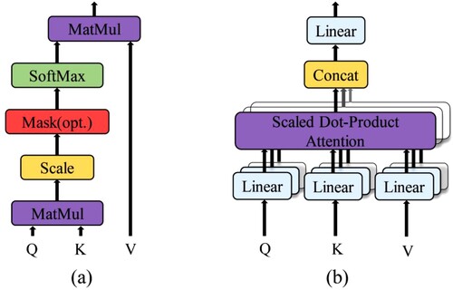
The functionality of a transformer depends heavily on the multi-head attention (MA) layer stacking and fusion (Wang et al. 2018), as shown in Figure 1. The scaled dot-product attention module in MA expresses the dependencies between tokens using self-attention, and the token obtained from the output of the embedding layer is linearly transformed to obtain Q, K, and V. The difference in the extraction of Q, K, V is that the weights of the linear transformation matrix are different. As shown in Eq. (1), Q and K are multiplied by the dot product to obtain the dependencies between the input tokens, and then the final self-attention matrix is obtained after the scale transformation, mask, and softmax operations. Multi-head attention then uses the number of heads, n, to further divide the learned Q, K, and V into n portions to learn different features, and finally splice them together as in Eqs. (2) and (3). Hence, in this process, each token is interrelated and the weight size of each token is learned, which is beneficial to solve global long-dependency problems. (1) $\mathrm{A}\mathrm{t}\mathrm{t}\mathrm{e}\mathrm{n}\mathrm{t}\mathrm{i}\mathrm{o}\mathrm{n}\left(Q,K,V\right)=\mathrm{s}\mathrm{o}\mathrm{f}\mathrm{t}\mathrm{m}\mathrm{a}\mathrm{x}\left({\displaystyle \frac{Q{K}^T}{\sqrt{d_k}}}\right)V$(1) (2) $\mathrm{h}\mathrm{e}\mathrm{a}{\mathrm{d}}_i=\mathrm{A}\mathrm{t}\mathrm{t}\mathrm{e}\mathrm{n}\mathrm{t}\mathrm{i}\mathrm{o}\mathrm{n}\left(Q{W}_i^Q,K{W}_i^K,V{W}_i^V\right)$(2) (3) $\mathrm{M}\mathrm{u}\mathrm{l}\mathrm{t}\mathrm{i}\mathrm{H}\mathrm{e}\mathrm{a}\mathrm{d}\left(Q,K,V\right)=\mathrm{C}\mathrm{o}\mathrm{n}\mathrm{c}\mathrm{a}\mathrm{t}\left(\mathrm{h}\mathrm{e}\mathrm{a}\mathrm{d}{}_1,\dots ,\mathrm{h}\mathrm{e}\mathrm{a}\mathrm{d}{}_n\right)W^O$(3)

Figure 1. Attention mechanism of the transformer. (a) Scaled dot-product attention module. (b) Multi-head attention mechanism.

2.2. Brief review of CNNs

A CNN mainly uses convolutional layers to extract image information. Each convolutional layer consists of multiple convolution kernels, which act on the local area of the image to obtain local patch size information through fixed-size convolution kernels. One convolution kernel can scan the entire image to achieve weight sharing and thus reduce network complexity (LeCun et al. 1999).

The 2D convolution operation is expressed as follows: (4) $v_{ij}^{xy}=f\left(\sum _{p=0}^{P_i-1}\sum _{q=0}^{Q_i-1}{k}_{ijm}^{pq}{v}_{\left(i-1\right)m}^{\left(x+p\right)\left(y+q\right)}+b_{ij}\right),$(4) where i denotes the position index in the convolutional layer, j denotes the position index of feature maps in the layer, $v_{ij}^{xy}$ denotes the eigenvalue of the j-th feature map in the i-th layer at (x, y), $b_{ij}$ is the offset, m is the index of all feature maps connected to the current layer from the previous convolutional layer, $k_{ijm}^{pq}$ is the weight of the m-th convolution kernel at (p, q), $P_i$ is the height of the convolution kernel, $Q_i$ is the width of the convolution kernel, and f is the activation function of the convolutional layer.

To combine spatial-spectral features and process HSI data, the 3D convolution operation (Ji et al. 2013) is introduced, which is calculated as follows: (5) $v_{ji}^{xyz}=f\left(\sum _{p=0}^{P_i-1}\sum _{q=0}^{Q_i-1}\sum _{r=0}^{R_i-1}{k}_{ijm}^{pqr}{V}_{\left(i-1\right)m}^{\left(x+p\right)\left(y+q\right)\left(z+r\right)}+b_{ij}\right)$(5) where $R_i$ denotes the size of the convolution kernel in the spectral dimension and the output of the 3D convolution operation retains the 3D volume shape of the input spectral information. The size of the output layer after the convolution operation is shown in Eq. (6): (6) $N=1+{\displaystyle \frac{W+2\times \mathrm{p}-1-\mathrm{d}\times \left(\mathrm{k}-1\right)}{\mathrm{s}}}$(6) where N denotes the output image size, W denotes the input image size, p is the padding size of the input feature map, d is the padding size of the convolution kernel defaulted to 1, k is the convolution kernel’s size, and s is the convolution kernel’s move step.

2.3. Overview of MDvT

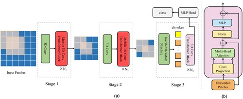
The mobile 3D convolutional vision transformer (MDvT) is a CvT-based backbone network that focuses on exploiting spatial-spectral information to make it suitable for the accurate classification of HSI. The MDvT hosts three modules – 3D convolution, mobile 3D convolution transformer block (MCTB) (Mehta and Rastegari 2021), and inverted residual structure (IRS) (Sandler et al. 2018) – which reduce the problems of the dramatic increase in the number of parameters and decrease in model speed brought about by the introduction of 3D convolution while fully utilizing the spectral information. The number of parameters in the self-attention mechanism are reduced by MCTB, and IRS reduces the number of parameters brought by 3D convolution to streamline the model and reach the optimal model state with the loss of as little accuracy as possible.

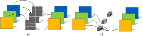
As shown in Figure 2, the MDvT draws on the structural design of the multi-stage hierarchy of CvT, which consists of three stages in total. Each stage comprises two parts. First, the 3D convolutional layer performs a down-sampling operation on the feature layer, and then the output result of the convolution operation is transformed into a token form acceptable to the transformer for self-attention learning. Figure 2b shows the transformer block of the last stage, which differs from that in stages 1 and 2 in that it uses depthwise separable convolution instead of linear mapping.

Figure 2. Network overview diagram of MDvT. MDvT consists of three core components: 3D convolution, mobile 3D convolution transformer block, and inverted residual structure.

2.4. Mobile 3D convolution transformer block

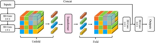
The MCTB is one of the core modules of the model, designed to accelerate the modeling of local and global information of the input tensor. The feature map is first modeled with local features through a 3 × 3 convolutional layer, and then the number of channels is adjusted through a 1 × 1 convolutional layer. The data are then immediately adjusted to token format by an ‘unfold’ operation and fed into the transformer for global feature extraction. A ‘fold’ operation then converts the token into a format that can be processed by the convolutional layer, and the number of channels is adjusted back to the original size through a 1 × 1 convolutional layer. Along the channel direction, the output result is concatenated with the original input feature map, and eventually a 3 × 3 convolutional layer is employed for feature fusion. It is worth noting that the data size does not change during the entire process.

For ordinary self-attention computation, it is generally straightforward to flatten the H and W dimensions to get a token sequence, i.e. [N, H, W, C] → [N, H*W, C], where N is the batch size, H is the height of the feature map, W is the width, and C is the number of convolution kernels. However, in MCTB, the 3D convolution layer is first introduced so that the input data becomes [N, C, H, W, B] (B is the number of bands); a square with side length 2 is also used to continue dividing the H, W, and B directions of the feature map, as shown in Figure 3, so the dimension of the token sequence becomes [N*8, H*W*B/8, C]. Each token only performs self-attention with a token of the same color, so the theoretical computational cost of attention is 1/8 of the original. Thus, the MCTB reduces the amount of data input to the transformer, greatly increasing the speed of the model run.

Figure 3. Diagram of the mobile 3D convolution transformer block.

2.5. Inverted residual structure

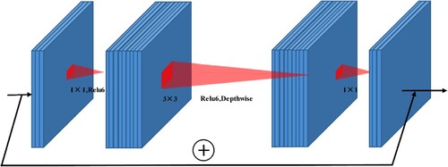
The inverted residual structure is designed to satisfy full information mining under the input condition of low-dimensional data, aiming to achieve a balance in terms of data volume and extraction efficiency. As shown in Figure 4, a 1 × 1 convolutional layer is first used to map the low-dimensional information to higher dimensions, then depthwise separable (DS) convolution is used to learn the feature information, and finally a 1 × 1 convolutional layer restores the number of convolution kernels to the size of the input. If the input and output data dimensions are the same, a shortcut operation is added. The activation function uses the Relu6 function, and the final layer of IRS uses a linear activation function to reduce the large loss of low-dimensional feature information caused by the Relu6 function (Sandler et al. 2018).

Figure 4. Diagram of the inverted residual structure.

Compared with traditional convolution operations, DS convolution substantially reduces the number of convolution operation parameters. As shown in Figure 5, DS convolution comprises two parts. Figure 5a shows that the depth of the convolution kernel of depthwise convolution is 1, and each convolution kernel only performs the convolution operation with one channel of the input matrix. Figure 5b shows that the size of the convolution kernel of pointwise convolution is 1 × 1, and the depth of the convolution kernel is equal to the channel of the input feature matrix. Therefore, the computation cost of DS convolution is $D_f^2\cdot D_m\left(D_k^2+D_n\right)$, where $D_f$ denotes the size of the input feature matrix, $D_m$ denotes the channel depth of the input feature matrix, $D_k$ denotes the size of the convolution kernel, and $D_n$ denotes the channel depth of the output feature matrix. The computational cost of the standard convolutional layer is $D_f^2\cdot D_m\left(D_k^2\cdot D_n\right)$; in general, $D_k$ is equal to 3, so the number of parameters in ordinary convolution is 8–9 times that in DS convolution. This is also valid for 3D convolutional layers, thereby reducing the model parameters with reduced accuracy loss.

Figure 5. Diagrams demonstrating depthwise separable convolution. (a) Depthwise convolution. (b) Pointwise convolution.

3. Experimental setup

3.1. Data description

This study used four publicly available HSI datasets. Among them, the WHU-Hi dataset (Zhong et al. 2018; Zhong et al. 2020) produced by Wuhan University from a Research study located on the Jianghan Plain of Hubei Province, China, with flat topography and abundant crop species.

The WHU-Hi-HongHu dataset comprised a complex agricultural scene with crop categories including different species of the same crop. The image has a spatial resolution of about 0.043 m, a size of 940 × 475 pixels, and 270 bands in the 400–1000 nm band coverage range. There were 22 major survey categories in the entire study scene.

The WHU-Hi-HanChuan dataset comprised an urban-rural fringe with buildings, water, and arable land containing seven crops, including strawberries, cowpeas, and soybeans. The image has a spatial resolution of about 0.109 m, a size of 1217 × 303 pixels, and 274 bands in the 400–1000 nm band coverage range. The presence of many shadow-covered areas in the images also posed a challenge for the correct differentiation of classes. There were 16 major survey categories in the entire study scene.

The WHU-Hi-LongKou dataset comprised a simple agricultural scenario containing six crop species: maize, cotton, sesame, broad-leaf soybean, narrow-leaf soybean, and rice. The image has a spatial resolution of about 0.463 m, a size of 550 × 400 pixels, and 270 bands in the 400–1000 nm band coverage range. There were nine major survey categories in the entire study scene.

The Pavia University dataset was acquired by the Reflection Optical System Imaging Spectrometer (ROSIS) sensor in the city of Pavia, Italy. The image has a spatial resolution of about 1.3 m, a size of 610 × 340 pixels, and 103 bands in the 430–860 nm band coverage range. There were nine major survey categories in the entire study scene. Table 1 lists the four datasets’ specific categories as well as the associated numbers of training and testing sets.

Table 1. Summary of category information for the HSI dataset.

Dataset	Class No.	Class Name	Training samples	Testing samples	Class No.	Class Name	Training samples	Testing samples
WHU-Hi-HongHu	0	Red roof	100	929	11	Brassica chinensis	100	590
	1	Road	100	227	12	Small Brassica chinensis	100	1493
	2	Bare soil	100	1448	13	Lactuca sativa	100	483
	3	Cotton	100	10879	14	Celtuce	100	60
	4	Cotton firewood	100	407	15	Film covered lettuce	100	477
	5	Rape	100	2963	16	Romaine lettuce	100	194
	6	Chinese cabbage	100	1600	17	Carrot	100	207
	7	Pakchoi	100	263	18	White radish	100	574
	8	Cabbage	100	714	19	Garlic sprout	100	225
	9	Tuber mustard	100	819	20	Broad bean	100	81
	10	Brassica parachinensis	100	727	21	Tree	100	262
WHU-Hi-HanChuan	0	Strawberry	100	4463	8	Grass	100	936
	1	Cowpea	100	2265	9	Red roof	100	1041
	2	Soybean	100	1018	10	Gray roof	100	1681
	3	Sorghum	100	525	11	Plastic	100	357
	4	Water spinach	100	110	12	Bare soil	100	901
	5	Watermelon	100	443	13	Road	100	1846
	6	Greens	100	580	14	Bright object	100	103
	7	Trees	100	1787	15	Water	100	7530
WHU-Hi-LongKou	0	Corn	100	3441	5	Rice	100	1175
	1	Cotton	100	827	6	Water	100	6695
	2	Sesame	100	293	7	Roads and houses	100	702
	3	Broad-leaf soybean	100	6311	8	Mixed weed	100	512
	4	Narrow-leaf soybean	100	405
Pavia-University	0	Asphalt	100	3265	5	Bare Soil	100	2464
	1	Meadows	100	9274	6	Bitumen	100	615
	2	Gravel	100	999	7	Bricks	100	1791
	3	Trees	100	1482	8	Shadow	100	423
	4	Metal Sheets	100	622

3.2. Comparison algorithms

Eight representative backbone networks were selected as the comparison strategies for HSI classification, including the machine learning method RF, classical CNN network, transformer, and transformer’s deformation. The specific setup parameters of the above models were as follows.

1. For RF, 200 decision trees were set in the experiments.

2. The 3D CNN architecture had seven convolutional blocks. Each convolutional block consisted of a convolutional layer, batch normalization layer, and Relu activation function. The convolution kernel’s size was 3 × 3 × 7 and the number of channels was set to [64, 128, 256].

3. For Resnet, with 34 layers of depth, the convolution kernel’s size included two types, 3 × 3 and 7 × 7, and the number of channels was set to [64, 128, 256, 512]. Compared with conventional CNN, the residual structure was added to prevent model degradation caused by too-deep layers of the network.

4. For ViT, only the encoder module of the transformer was used; its depth was 12, the number of heads was 10, and the token dimension of the transformer was 128.

5. For CvT, the convolution kernel’s size was 3 × 3, stride was 2, number of channels was [64, 128, 256], depth of the transformer was [2, 4, 6], and number of heads was [2, 4, 4] in order.

6. For CvT3D, the convolution kernel’s size was 3 × 3 × 3, and the rest of the parameter settings were the same as for the CvT model.

7. The SpectralFormer is a variant of the ViT-based model. It introduced groupwise spectral embedding (GSE) to exploit spectral information and used cross-layer adaptive fusion (CAF) to achieve cross-layer information transfer. The band patch’s size was 7, and the rest of the parameter settings were the same as for the ViT model.

8. For A²S²K-ResNet (Roy et al. 2021), jointed extraction of spectral-space features using improved 3D ResBlocks with an efficient feature recalibration (EFR) mechanism to improve classification performance. The patch size was 15, and the rest of the parameter settings were the same as for its original papers.

9. For the MDvT model proposed in this paper, the design guidelines of ViT and CvT were followed, and the parameters of the model were set to be the same as those of CvT3D.

Models of neural networks were implemented under the PyTorch framework, and the workstation used was mainly Google’s free Colaboratory platform with a built-in NVIDIA Tesla T4 12.68 GB GPU. The optimizer used in the above neural network models was AdamW (Loshchilov and Hutter 2017), the initial learning rate (lr) was 5e⁻⁴, the lr was adjusted once every 10 iterations, with each update of 0.9 times the lr, and the number of epochs was 200. For both the CNN model and its hybrid model, the value of the patch size was 15. Owing to the huge amount of HSI data and the pressure of calculation, the data was preprocessed and the number of spectral bands was limited to 100 using principal component analysis (Yue et al. 2015) for dimensionality reduction. Finally, the categorization findings were quantitatively assessed using the overall accuracy (OA), average accuracy (AA), and Kappa coefficient. To verify the validity of the method, each experiment was repeated ten times to obtain the average precision and standard deviation.

4. Results

The classification maps of the WHU-Hi-HongHu dataset obtained using MDvT and other comparison methods are shown in Figure 6, and the specific accuracy evaluations are presented in Table 2. The results of RF (Figure 6c) shows many regional misclassifications owing to the similarity in spectral information of different crops and severe within-class spectral variability in HSI. For instance, there was a significant misinterpretation between bare soil and cotton firewood, and small Brassica chinensis and rape. Compared to the machine learning approach, deep learning methods showed significant improvements in HSI classification. The 3D CNN (Figure 6d) and Resnet (Figure 6e) maps also show many misclassified areas, but OA was improved by 36.61% and 37.65%, respectively, compared with RF. Because these methods only obtain the information of local patches and fail to make full use of global dependencies, the classification results showed more fragmented blocks. However, the ViT model can solve the problem of global dependencies, and the fragmented regions in the classification results (Figure 6f) were significantly reduced. The CvT model integrates the convolutional layer of the hierarchical structure based on ViT, and the OA was improved by 3.16% compared with ViT. Meanwhile, CvT3D replaces the 2D convolution operation of CvT with 3D convolution, and the fragmentation of the classification results (Figure 6h) was further reduced compared with CvT, but the OA was reduced. The SpectralFormer model introduces spectral embedding and cross-layer fusion modules, making fuller use of spectral-spatial information compared to ViT, and the OA was improved by 2.91%. The A²S²K-ResNet has an adaptive spectral spatial information discrimination mechanism, and the OA was improved by 8.37%. The experiment results show that the introduction of spectral dimension in the base model will effectively improve the HSI classification accuracy. From both a visual perspective and in terms of quantitative analysis, MDvT achieves the best accuracy, showing that the introduced IRS and MCTB modules can better integrate 3D convolution into the transformer.

Figure 6. Results of classification from the WHU-Hi-HongHu dataset using various models. (a) True color image (R: band 108, G: band 68, and B: band 32). (b) Ground-truth image. (c) RF. (d) 3D CNN. (e) Resnet. (f) ViT. (g) CvT. (h) CvT3D. (i) SpectralFormer. (j) A²S²K-ResNet. (k) MDvT.

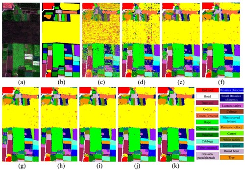
Table 2. Accuracy of classification for the WHU-Hi-HongHu dataset. The most outstanding results for each class are highlighted in bold.

Class No.	RF	3D CNN	Resnet	ViT	CvT	CvT3D	SpectralFormer	A^2S^2K-ResNet	MDvT
1	86.62 ± 0.540	85.67 ± 0.495	94.60 ± 0.390	98.25 ± 0.395	97.22 ± 0.690	97.48 ± 0.091	98.14 ± 0.160	97.95 ± 0.385	98.14 ± 0.325
2	43.94 ± 0.109	76.96 ± 0.275	85.17 ± 1.270	80.08 ± 0.075	98.62 ± 0.720	92.71 ± 0.245	89.33 ± 0.925	94.49 ± 0.960	100.00 ± 0.000
3	92.24 ± 0.190	98.08 ± 0.445	98.62 ± 0.405	99.86 ± 0.185	99.31 ± 0.045	100.00 ± 0.00	99.93 ± 0.021	100.00 ± 0.000	99.93 ± 0.035
4	90.47 ± 0.465	92.83 ± 0.082	97.48 ± 1.085	99.75 ± 0.010	98.43 ± 0.625	99.73 ± 0.074	99.51 ± 0.050	99.99 ± 0.000	99.89 ± 0.045
5	16.61 ± 0.025	67.59 ± 0.995	80.09 ± 0.445	51.02 ± 0.505	72.64 ± 0.395	71.20 ± 0.049	71.76 ± 1.320	78.42 ± 0.815	88.86 ± 0.395
6	17.18 ± 0.115	82.35 ± 0.039	76.71 ± 0.080	80.21 ± 1.865	87.17 ± 0.595	44.87 ± 0.610	76.24 ± 0.705	78.46 ± 0.300	90.85 ± 0.280
7	41.15 ± 0.131	62.94 ± 0.360	92.24 ± 0.105	82.01 ± 1.005	92.70 ± 0.440	93.94 ± 0.080	93.73 ± 0.640	94.87 ± 0.595	94.05 ± 0.065
8	8.71 ± 0.365	49.68 ± 0.760	40.38 ± 0.290	39.35 ± 0.652	63.25 ± 0.305	72.19 ± 0.025	68.52 ± 0.355	75.60 ± 0.835	77.25 ± 0.075
9	76.95 ± 0.895	86.23 ± 1.460	100.00 ± 0.000	99.79 ± 0.030	100.00 ± 0.000	97.55 ± 0.026	100.00 ± 0.000	100.00 ± 0.000	99.85 ± 0.125
10	24.73 ± 0.550	84.87 ± 2.080	59.51 ± 0.505	76.27 ± 1.095	86.25 ± 0.520	78.29 ± 0.570	92.22 ± 1.435	96.54 ± 0.180	87.58 ± 0.235
11	8.63 ± 0.240	73.53 ± 0.084	85.25 ± 0.055	83.84 ± 1.520	82.45 ± 1.105	69.32 ± 0.575	85.78 ± 0.605	83.49 ± 0.080	84.63 ± 1.305
12	8.73 ± 1.370	64.91 ± 0.545	67.92 ± 0.155	38.14 ± 0.280	48.18 ± 0.840	47.11 ± 0.865	60.97 ± 1.035	74.57 ± 1.545	58.12 ± 0.090
13	15.48 ± 0.305	43.02 ± 0.940	30.89 ± 0.970	29.95 ± 1.245	38.60 ± 0.890	30.71 ± 0.135	33.68 ± 1.030	42.04 ± 0.215	45.93 ± 0.400
14	51.57 ± 1.020	62.46 ± 1.005	59.17 ± 0.740	94.37 ± 1.140	94.02 ± 0.320	79.61 ± 0.285	94.18 ± 0.795	97.78 ± 0.155	93.13 ± 0.565
15	4.14 ± 0.300	58.00 ± 0.055	76.92 ± 0.240	100.00 ± 0.000	95.24 ± 0.155	92.31 ± 0.795	100.00 ± 0.000	93.75 ± 0.730	100.00 ± 0.000
16	72.56 ± 0.450	99.17 ± 0.110	96.25 ± 0.575	98.94 ± 0.210	98.55 ± 0.620	100.00 ± 0.000	100.00 ± 0.000	99.58 ± 0.005	99.58 ± 0.015
17	51.98 ± 0.875	100.00 ± 0.000	91.51 ± 0.245	84.72 ± 0.505	99.49 ± 0.175	87.39 ± 0.295	100.00 ± 0.000	96.52 ± 0.092	99.49 ± 0.255
18	12.34 ± 0.140	82.63 ± 0.420	67.70 ± 0.905	56.69 ± 0.850	63.49 ± 0.745	69.18 ± 0.062	67.54 ± 0.690	61.18 ± 0.455	65.08 ± 0.645
19	42.14 ± 0.580	78.91 ± 0.585	53.06 ± 0.635	71.58 ± 1.780	63.06 ± 1.505	67.27 ± 0.180	66.75 ± 0.250	88.59 ± 0.665	92.21 ± 0.855
20	21.13 ± 0.320	17.87 ± 0.575	72.76 ± 0.910	69.72 ± 1.135	81.72 ± 1.005	76.84 ± 0.028	57.94 ± 1.065	83.77 ± 0.455	92.59 ± 0.575
21	10.79 ± 0.700	98.78 ± 0.295	48.80 ± 0.950	55.00 ± 0.650	92.77 ± 0.88	87.10 ± 0.875	94.19 ± 1.070	96.42 ± 1.002	100.00 ± 0.000
22	4.41 ± 0.120	74.64 ± 0.042	54.84 ± 0.920	47.99 ± 0.940	46.55 ± 0.750	49.51 ± 0.605	54.26 ± 0.725	74.43 ± 1.700	83.60 ± 0.375
OA (%)	41.83 ± 0.255	78.44 ± 0.505	79.48 ± 0.550	81.14 ± 0.290	85.3 ± 0.605	81.90 ± 0.015	84.05 ± 0.415	87.85 ± 0.805	90.20 ± 0.106
AA (%)	48.33 ± 0.210	85.11 ± 0.495	80.99 ± 0.500	83.54 ± 0.095	85.52 ± 0.595	86.20 ± 0.040	87.35 ± 0.340	92.23 ± 0.440	92.33 ± 0.225
Kappa (%)	33.91 ± 0.170	73.23 ± 0.410	74.20 ± 0.545	76.43 ± 0.365	81.51 ± 0.710	77.37 ± 0.035	80.02 ± 0.140	84.75 ± 0.580	87.66 ± 0.115

The classification maps of the WHU-Hi-HanChuan dataset obtained using MDvT and other comparison methods are shown in Figure 7, and the specific accuracy evaluations are presented in Table 3. Shadow patches were prevalent in the image because the WHU-Hi-HanChuan dataset was collected in the afternoon when the sun’s elevation angle was low, and compared to places with typical illumination, those locations displayed extremely low brightness. For RF method, the classification results showed a large number of misclassified regions (Figure 7c). The 3D CNN method does not include a maxing pooling layer, dropout layer, or other ways to enhance the operation of model generalization, so a serious fragmentation phenomenon was present (Figure 7d). In Resent, soybean and gray roof, and soybean and cowpea also showed serious misclassifications. Compared with RF, the OA of CvT and CvT3D improved by 25.52% and 23.27%, respectively, but misclassification still occurred in shaded coverage areas. For ViT, SpectralFormer and A²S²K-ResNet methods, overall they have achieved high precision performance. However, compared with MDvT, there are still fragmented regions, which is due to the multi-scale feature extraction of MDvT, which has a higher advantage for the recognition of spectrally similar features.

Figure 7. Results of classification from the WHU-Hi-HanChuan dataset using various models. (a) True color image (R: band 108, G: band 68, and B: band 32). (b) Ground-truth image. (c) RF. (d) 3D CNN. (e) Resnet. (f) ViT. (g) CvT. (h) CvT3D. (i) SpectralFormer. (j) A²S²K-ResNet. (k) MDvT.

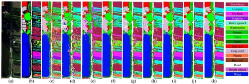
Table 3. Accuracy of classification for the WHU-Hi-HanChuan dataset. The most outstanding results for each class are highlighted in bold.

Class No.	RF	3D CNN	Resnet	ViT	CvT	CvT3D	SpectralFormer	A^2S^2K-ResNet	MDvT
1	95.30 ± 0.070	95.34 ± 0.570	94.62 ± 0.170	98.88 ± 0.200	98.45 ± 0.025	97.73 ± 0.260	98.74 ± 0.785	97.64 ± 0.478	99.66 ± 0.009
2	69.91 ± 0.025	81.7 ± 0.290	97.31 ± 0.720	94.47 ± 0.460	95.64 ± 0.630	92.34 ± 1.700	94.76 ± 0.200	94.09 ± 0.630	96.27 ± 0.165
3	36.12 ± 0.090	75.13 ± 0.860	40.59 ± 0.375	72.55 ± 1.365	77.97 ± 1.096	83.23 ± 0.145	88.40 ± 0.045	89.84 ± 0.096	90.95 ± 0.075
4	83.49 ± 0.410	99.19 ± 0.260	97.68 ± 0.310	100.00 ± 0.000	95.49 ± 0.134	100.00 ± 0.00	100.00 ± 0.000	100.00 ± 0.000	100.00 ± 0.000
5	11.59 ± 0.705	90.16 ± 1.831	99.1 ± 0.430	84.62 ± 0.070	95.65 ± 0.830	94.02 ± 0.990	100.00 ± 0.000	90.16 ± 0.830	100.00 ± 0.000
6	20.11 ± 1.395	73.63 ± 0.305	94.79 ± 0.500	74.26 ± 0.475	77.70 ± 0.408	86.84 ± 0.260	80.04 ± 0.735	89.08 ± 0.408	84.41 ± 0.005
7	46.38 ± 0.700	91.77 ± 0.325	54.46 ± 0.675	88.82 ± 1.445	68.16 ± 0.450	98.14 ± 0.205	99.15 ± 0.085	85.04 ± 0.450	95.78 ± 0.005
8	32.67 ± 1.810	77.47 ± 1.945	99.2 ± 0.160	98.44 ± 0.285	84.50 ± 0.523	87.63 ± 0.590	86.58 ± 0.445	96.94 ± 0.523	89.94 ± 0.025
9	84.98 ± 0.125	73.98 ± 0.860	72.37 ± 0.265	83.77 ± 0.125	86.28 ± 0.128	78.20 ± 0.115	82.10 ± 0.115	90.86 ± 1.128	87.64 ± 0.015
10	85.3 ± 1.155	93.02 ± 0.925	94.03 ± 0.015	95.86 ± 0.895	98.76 ± 0.319	97.75 ± 0.235	97.29 ± 0.115	90.76 ± 0.319	96.51 ± 0.002
11	45.21 ± 0.785	60.16 ± 0.108	82.41 ± 0.825	79.19 ± 0.730	87.87 ± 0.916	72.54 ± 0.760	76.16 ± 0.110	72.95 ± 0.916	76.25 ± 0.020
12	23.53 ± 0.005	94.76 ± 1.510	99.05 ± 0.085	98.04 ± 0.285	93.67 ± 0.014	76.12 ± 0.695	96.18 ± 0.072	100.00 ± 0.000	99.58 ± 0.007
13	66.02 ± 0.86	69.53 ± 0.130	84.86 ± 0.210	91.13 ± 0.020	93.70 ± 0.813	69.64 ± 1.240	89.64 ± 0.120	97.30 ± 0.813	93.04 ± 0.005
14	92.42 ± 0.655	96.09 ± 1.590	99.77 ± 0.170	99.83 ± 0.060	98.03 ± 0.325	99.35 ± 0.075	99.72 ± 0.045	100.00 ± 0.000	99.59 ± 0.001
15	35.43 ± 0.070	88.03 ± 0.985	100.00 ± 0.000	97.92 ± 0.515	87.00 ± 0.274	93.24 ± 0.640	100.00 ± 0.000	95.37 ± 0.274	100.00 ± 0.000
16	99.66 ± 0.005	99.65 ± 0.355	98.47 ± 0.415	99.97 ± 0.005	99.92 ± 0.014	100.00 ± 0.000	99.93 ± 0.003	99.94 ± 0.004	100.00 ± 0.000
OA (%)	68.39 ± 0.100	87.2 ± 0.315	87.56 ± 1.650	94.06 ± 0.335	93.91 ± 0.593	91.66 ± 0.710	94.22 ± 0.335	94.51 ± 0.393	95.27 ± 0.082
AA (%)	67.19 ± 0.300	85.42 ± 0.695	82.83 ± 0.570	93.17 ± 0.505	89.72 ± 0.344	91.22 ± 0.665	92.91 ± 0.175	95.13 ± 0.244	95.35 ± 0.015
Kappa (%)	64.07 ± 0.120	85.16 ± 0.215	85.48 ± 1.015	93.07 ± 0.395	92.89 ± 0.299	90.32 ± 0.355	93.26 ± 0.205	93.61 ± 0.199	0.9449 ± 0.023

The classification maps of the WHU-Hi-LongKou dataset obtained using MDvT and other comparison methods are shown in Figure 8, and the specific accuracy evaluations are presented in Table 4. Compared with the two previous datasets, the WHU-Hi-LongKou dataset is relatively simple and has more obvious interclass characteristics. The OA of RF reached 87.85%. However, no contextual information was combined, and fragmentation and misclassification were still evident. For example, cotton and broad-leaf soybean, and corn and mixed weeds were distinguished with low accuracy (Figure 8c). The 3D CNN map also exhibited large blocks of misclassification (Figure 8d), while the Resnet classification results showed small patches of broad-leaf soybean identified as narrow-leaf soybean (Figure 8e). The transformer-based models all achieved high accuracy classification results, with the highest OA of 99.10% for MDvT. For the misclassification phenomenon of broad-leaf soybean and cotton, MDvT can also handle it well, indicating that the detailed extraction of local information and the fusion of global information can accurately separate the features.

Figure 8. Results of classification from the WHU-Hi – LongKou dataset using various models. (a) True color image (R: band 108, G: band 68, and B: band 32). (b) Ground-truth image. (c) RF. (d) 3D CNN. (e) Resnet. (f) ViT. (g) CvT. (h) CvT3D. (i) SpectralFormer. (j) A²S²K-ResNet. (k) MDvT.

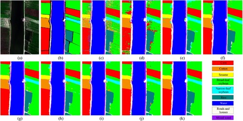
Table 4. Accuracy of classification for the WHU-Hi – LongKou dataset. The most outstanding results for each class are highlighted in bold.

Class No.	RF	3D CNN	Resnet	ViT	CvT	CvT3D	SpectralFormer	A^2S^2K-ResNet	MDvT
1	96.39 ± 0.100	99.14 ± 0.350	95.44 ± 0.225	99.65 ± 0.115	94.27 ± 0.315	99.02 ± 0.470	96.88 ± 0.015	98.15 ± 0.230	98.54 ± 0.115
2	55.13 ± 2.295	75.09 ± 1.455	100.00 ± 0.000	82.25 ± 0.005	98.25 ± 0.385	96.61 ± 1.025	86.44 ± 0.335	99.76 ± 0.125	100.00 ± 0.000
3	36.36 ± 1.045	93.87 ± 0.720	86.43 ± 1.910	95.75 ± 0.315	87.72 ± 1.495	80.05 ± 0.380	86.69 ± 0.000	99.66 ± 0.005	97.02 ± 0.315
4	99.48 ± 0.010	95.03 ± 0.385	99.80 ± 0.037	99.88 ± 0.035	99.80 ± 0.010	99.46 ± 0.145	99.98 ± 0.000	99.98 ± 0.001	100.00 ± 0.000
5	42.46 ± 3.14	94.35 ± 0.195	31.96 ± 1.760	75.00 ± 0.140	71.55 ± 0.445	73.24 ± 1.770	43.69 ± 0.190	100.00 ± 0.000	81.00 ± 0.140
6	97.90 ± 0.400	95.83 ± 1.740	99.31 ± 0.460	99.58 ± 0.210	100.00 ± 0.000	99.91 ± 0.045	100.00 ± 0.000	100.00 ± 0.000	100.00 ± 0.000
7	100.00 ± 0.000	98.91 ± 0.053	99.97 ± 0.025	99.79 ± 0.105	100.00 ± 0.000	100.00 ± 0.000	100.00 ± 0.000	98.870 ± 0.320	99.87 ± 0.105
8	76.62 ± 1.100	67.39 ± 1.725	94.84 ± 0.195	93.72 ± 0.575	93.93 ± 0.680	99.85 ± 0.065	98.72 ± 0.070	97.90 ± 0.675	98.31 ± 0.575
9	51.99 ± 1.120	84.37 ± 1.06	92.49 ± 0.785	95.51 ± 0.365	95.34 ± 0.230	96.39 ± 0.025	90.07 ± 0.090	79.37 ± 0.690	98.61 ± 0.365
OA (%)	88.45 ± 0.020	94.41 ± 0.208	94.25 ± 0.630	97.87 ± 0.110	97.51 ± 0.415	98.35 ± 0.295	95.75 ± 0.035	98.58 ± 0.145	99.10 ± 0.110
AA (%)	91.21 ± 0.180	94.31 ± 0.705	95.72 ± 1.360	98.88 ± 0.010	98.3 ± 0.220	98.37 ± 0.520	97.67 ± 0.005	97.83 ± 0.370	99.18 ± 0.010
Kappa (%)	85.31 ± 0.030	92.69 ± 0.165	92.56 ± 0.830	98.88 ± 0.020	96.74 ± 0.215	97.84 ± 0.390	94.48 ± 0.045	98.13 ± 0.115	98.82 ± 0.145

The classification maps of the Pavia University dataset obtained using MDvT and other comparison methods are shown in Figure 9 and the specific accuracy evaluations are presented in Table 5. Deep learning does improve the pretzel phenomenon compared to the machine learning approach. But misclassification and fragmentation are still serious. Compared with CvT3D, MDvT incorporates a variety of advanced modules that can better balance spectral and spatial information, thus alleviating the misclassification problem caused by spectral similarity. Compared to A²S²K-ResNet, the basic CNN and transformer framework in MDvT acquires global texture information and detailed abstraction information, so the performance is in the leading position.

Figure 9. Results of classification from the Pavia University dataset using various models. (a) True color image (R: band 55, G: band 7, and B: band 31). (b) Ground-truth image. (c) RF. (d) 3D CNN. (e) Resnet. (f) ViT. (g) CvT. (h) CvT3D. (i) SpectralFormer. (j) A²S²K-ResNet. (k) MDvT.

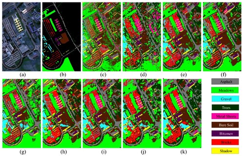
Table 5. Accuracy of classification for the Pavia University dataset. The most outstanding results for each class are highlighted in bold.

Class No.	RF	3D CNN	Resnet	ViT	CvT	CvT3D	SpectralFormer	A^2S^2K-ResNet	MDvT
1	95.96 ± 0.010	93.01 ± 0.720	91.55 ± 0.690	99.48 ± 0.040	95.29 ± 0.890	99.58 ± 0.025	98.08 ± 0.000	98.78 ± 0.090	99.84 ± 0.010
2	92.44 ± 0.340	97.86 ± 0.755	98.87 ± 0.080	99.74 ± 0.060	97.74 ± 0.420	98.72 ± 0.040	98.80 ± 0.000	99.72 ± 0.040	99.48 ± 0.130
3	55.77 ± 0.150	72.56 ± 0.810	70.23 ± 0.595	83.48 ± 2.105	84.86 ± 1.470	78.54 ± 1.410	80.15 ± 0.030	76.26 ± 0.820	98.66 ± 0.090
4	71.38 ± 0.380	62.85 ± 0.055	84.21 ± 0.405	97.06 ± 0.545	94.91 ± 0.215	95.71 ± 0.300	97.23 ± 0.035	97.98 ± 0.015	97.57 ± 0.410
5	98.11 ± 0.310	91.85 ± 0.290	99.68 ± 0.145	100.00 ± 0.000	99.36 ± 0.040	99.84 ± 0.080	99.20 ± 0.000	99.04 ± 0.480	99.68 ± 0.140
6	54.82 ± 1.045	84.44 ± 1.175	85.15 ± 0.090	95.21 ± 0.340	97.35 ± 1.875	96.73 ± 0.040	97.02 ± 0.000	99.23 ± 0.105	99.92 ± 0.045
7	52.61 ± 0.035	98.48 ± 1.955	65.91 ± 0.545	66.56 ± 4.085	89.91 ± 0.565	99.51 ± 0.070	93.60 ± 0.000	100.00 ± 0.000	99.35 ± 0.325
8	78.55 ± 0.340	72.83 ± 0.055	77.46 ± 0.270	91.53 ± 0.080	78.76 ± 0.155	92.37 ± 0.480	84.35 ± 0.020	92.52 ± 0.395	93.20 ± 0.225
9	80.88 ± 0.310	95.05 ± 0.130	91.96 ± 0.210	99.76 ± 0.030	87.55 ± 0.580	94.80 ± 0.630	99.05 ± 0.000	100.00 ± 0.000	100.00 ± 0.000
OA (%)	78.86 ± 0.330	87.36 ± 0.695	89.82 ± 0.655	95.92 ± 0.001	94.36 ± 0.665	96.67 ± 0.170	95.89 ± 0.005	97.31 ± 0.320	98.86 ± 0.115
AA (%)	84.61 ± 0.020	92.07 ± 0.405	91.47 ± 0.820	96.48 ± 0.110	93.60 ± 0.150	96.61 ± 0.315	95.83 ± 0.000	96.42 ± 0.160	98.59 ± 0.145
Kappa (%)	72.85 ± 0.355	83.60 ± 0.275	86.63 ± 0.575	94.59 ± 0.005	92.45 ± 0.815	95.55 ± 0.220	94.52 ± 0.005	96.42 ± 0.280	98.48 ± 0.073

5. Discussion

5.1. Sensitivity of training set size to classification results

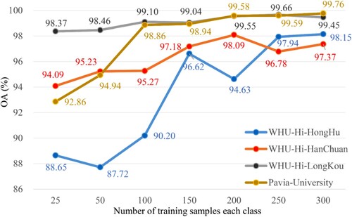
Owing to the complex structure of HSI data, the hierarchy of CNNs often needs a high amount of training samples to acquire valid information between categories, so a small amount of training data may lead to overfitting. For practical feature classification scenarios, labeled samples are often very limited, so finding ways to maximize the learning ability of the model with a small number of samples is an important issue in classification scenarios. As shown in Figure 10, the WHU-Hi and Pavia University datasets were used to evaluate the images of HSI classification results with different numbers of training samples. Each training sample was run ten times to obtain the average OA result and its standard deviation. As increasing the percentage of training samples, the OA tended to increase; it is also noteworthy that MDvT showed good classification performance with small samples of (25, 50) in the training set.

Figure 10. Effect of different number of training samples on MDvT in WHU-Hi and Pavia University datasets.

5.2. Impact of patch size on MDvT classification performance

It is well known that patch size is an important hyperparameter for CNN models(Jin et al. 2020). Different patch sizes have different degrees of influence on a model, and the findings indicate that adding the patch size appropriately can improve the accuracy of a model. However, too large an input data size may introduce additional noise, particularly when the pixels are situated towards the category’s boundaries, which could reduce accuracy (Zhang, Zhao, and Zhang 2020). Furthermore, the deep learning-based approach is inherently demanding on the chosen computational hardware, with overly large input data adding to the hardware burden and substantially increasing the training time and video memory usage. Using the WHU-Hi-HongHu dataset as an example, different patch sizes were selected to explore their effect on the MDvT’s categorization precision. According to the results in Table 6, the highest classification accuracy was achieved with an input size of 19 × 19. However, the training time and running memory of the model increase substantially as the input size increases. Compared with the 19 × 19 input size, the 15 × 15 input size lost 0.68% of OA, but the model training time was reduced by 42.37%. Therefore, we determined 15 × 15 to be the optimal patch size.

Table 6. Impact of patch size on MDvT classification performance. Time denotes the time required for the model to train an epoch. The most outstanding results are highlighted in bold.

Patch size	11	13	15	17	19
OA (%)	85.34	87.89	90.20	88.93	90.88
AA (%)	89.39	91.35	92.33	92.23	92.50
KAPPA	0.82	0.85	0.88	0.86	0.89
Time/s	24	33	34	57	59

5.3. Ablation study for the MDvT method

The addition of different modules (i.e. IRS and MCTB) to a network can improve model classification accuracy. Therefore, different modules were chosen to be added gradually to the network and the WHU-Hi-HongHu dataset was used to study their effectiveness for the HSI classification task. There are three stages in the MDvT model, each divided into two parts, and three different modules were added to the model to judge the classification performances of specific combinations. It is worth noting that the MCTB uses a square of length 2 to cut the data, so the minimum size of the input data must be ≥ 4. The common patch size value was 15, so the MCTB can be used at most twice in the entire model. From Table 7, it can be seen that using MCTB twice can improve the accuracy of the model by 5.74%–7.63%, greatly reduce the training time by 57.32%–60.92%, and improve the model training parameters. The number of model parameters can be reduced by IRS; for example, for CvT3IRS compared with the same configuration of CvT3D, the model parameters were reduced by 0.7 M, but the accuracy decreased by 0.78%–5.62%. The classification accuracy will be reduced by using IRS too much in MDvT. Therefore, 3D convolution is used for the input data of the first two stages, and IRS is used only in the last stage to limit the amount of MDvT parameters and control overfitting. Experimentally, the best classification efficiency is driven by the MDvT module combination in HSI, shortening the training time and limiting the number of model parameters while improving classification accuracy.

Table 7. Ablation experiments on the WHU-Hi-HongHu dataset with a CvT-based backbone model combined with different modules. Param denotes the training parameters of the model, and Time denotes the time required for the model to train an epoch. The most outstanding results are highlighted in bold.

Methods	Number of modules used			OA	AA	Kappa	Param (M)	Time/s
	3D convolution	IRS	MCTB
CvT3D	3	0	0	81.90	86.20	0.7737	7.24	82
CvT3D	3	0	1	86.41	89.33	0.8291	7.59	46
CvT3D	3	0	2	87.64	90.50	0.8448	8.31	35
CvT3IRS	0	3	0	80.79	82.10	0.7603	6.54	87
CvT3IRS	0	3	1	80.82	83.11	0.7645	6.89	46
CvT3IRS	0	3	2	88.42	90.23	0.8550	7.61	34
MDvT	1	2	1	83.69	85.16	0.7959	6.89	46
MDvT	1	2	2	85.86	87.85	0.8224	7.61	35
MDvT	2	1	1	85.70	87.98	0.8211	7.02	46
MDvT	2	1	2	90.20	92.33	0.8766	7.75	34

5.4. Deep feature visualization of MDvT

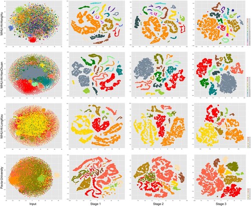
High-dimensional data are frequently visualized using the t-distributed stochastic neighbor embedding (t-SNE) technique (van der Maaten and Hinton 2008); it is capable of mapping data between high-dimensional and low-dimensional spaces, shorten the distance between similar categories, enlarge the gap between different instances, and keep the regional characteristics of the original data. To further understand the learning process within the MDvT model, the feature extraction results of the three stages in the model were visualized. As shown in Figure 11, the input data classes were highly similar to each other with serious overlap. After the output results of the first stage of the model, most of the classes were clearly distinguished, although there were still scattered clusters distributed in different regions. After the second stage, the same classes were closer to each other, but some confusion occurred between features with similar spectral information; for example, Chinese cabbage and Lactuca sativa in the WHU-Hi-HongHu dataset, plastic and road in the WHU-Hi-HanChuan dataset, narrow-leaf soybean and rice in the WHU-Hi-LongKou dataset, and Asphalt and Gravel in the Pavia University dataset. Following the third stage, the classification task was essentially complete, the distinction between classes was obvious, and the boundaries of each type of feature could clearly be seen (Figure 11).

Figure 11. Visualization of the distribution of categories in the feature maps of each stage of MDvT in the WHU-Hi and Pavia University datasets using t-SNE. The numbering of the categories in the figure corresponds to Table 1.

6. Conclusion

To fully utilize the spatial-spectral information of HSI, a new mobile 3D convolutional vision transformer network (MDvT) is proposed. The MDvT aims to meet the classification challenges of complex and diverse crop plots with highly similar spectral features. In MDvT, a layered hierarchy is used to combine multi-scale information while better adapting to global dependencies, thus improving the generalization ability of the model. Unlike ordinary CNNs that poorly mine and express the spectral features’ sequence characteristics, invoking 3D convolution pays full attention to spectral information. Lightweight modules (IRS and MCTB) are subsequently introduced to accelerate the model while taking into account the extraction of global features. Experimental results using the WHU-Hi dataset show that MDvT outperforms other classical classification models (e.g. Resnet, ViT, CvT, and others) and can provide high-performance results for HSI classification.

Our ablation experiments showed that the MDvT can still achieve class-leading levels of performance with small sample sizes. The IRS and MCTB modules reduced the number of model parameters, greatly speeding up the model run. For features with highly similar spectra, the model showed a notable ability to distinguish them in the first stage. The efficiency of HSI classification was improved by increasing the differences between complex categories.

In future research, lightweight models remain a focus of research in remote sensing classification tasks. The operation of reducing token sequence inter-multiplication in the MCTB module will be an important factor in improving the speed of MDvT runtime, and should be more widely used in the CNN and transformer hybrid model. In addition, we also hope to use more advanced techniques (e.g. weakly supervised learning and self-supervised learning) to further improve the hybrid architecture, reduce the dependence on samples, and improve the HSI classification performance.

Acknowledgement

The authors would especially like to thank Wuhan University and Pavia University for providing the open HSI dataset.

Disclosure statement

No potential conflict of interest was reported by the author(s).

References

- Adam, E., O. Mutanga, and D. Rugege. 2010. “Multispectral and Hyperspectral Remote Sensing for Identification and Mapping of Wetland Vegetation: A Review.” Wetlands Ecology and Management 18 (3): 281–296. doi:10.1007/s11273-009-9169-z.
- Bazi, Y., L. Bashmal, M. M. Al Rahhal, R. Al Dayil, and N. Al Ajlan. 2021. “Vision Transformers for Remote Sensing Image Classification.” Remote Sensing 13 (3): 516–534. doi:10.3390/rs13030516.
- Chen, Y. S., H. L. Jiang, C. Y. Li, X. P. Jia, and P. Ghamisi. 2016. “Deep Feature Extraction and Classification of Hyperspectral Images Based on Convolutional Neural Networks.” IEEE Transactions on Geoscience and Remote Sensing 54 (10): 6232–6251. doi:10.1109/TGRS.2016.2584107.
- Dalponte, M., H. O. Orka, T. Gobakken, D. Gianelle, and E. Naeesset. 2013. “Tree Species Classification in Boreal Forests With Hyperspectral Data.” IEEE Transactions on Geoscience and Remote Sensing 51 (5): 2632–2645. doi:10.1109/TGRS.2012.2216272.
- Devlin, Jacob, Ming-Wei Chang, Kenton Lee, and Kristina Toutanova. 2018. “Bert: Pre-training of Deep Bidirectional Transformers for Language Understanding.” arXiv preprint arXiv:1810.04805.
- Dosovitskiy, Alexey, Lucas Beyer, Alexander Kolesnikov, Dirk Weissenborn, Xiaohua Zhai, Thomas Unterthiner, Mostafa Dehghani, et al. 2020. “An Image is Worth 16(16 Words: Transformers for Image Recognition at Scale.” arXiv preprint arXiv:2010.11929.
- Fauvel, M., Y. Tarabalka, J. A. Benediktsson, J. Chanussot, and J. C. Tilton. 2013. “Advances in Spectral-Spatial Classification of Hyperspectral Images.” Proceedings of the IEEE 101 (3): 652–675. doi:10.1109/JPROC.2012.2197589.
- Gislason, Pall Oskar, Jon Atli Benediktsson, and Johannes R Sveinsson. 2006. “Random Forests for Land Cover Classification.” Pattern Recognition Letters 27 (4): 294–300. doi:10.1016/j.patrec.2005.08.011
- He, X., Y. S. Chen, and Z. H. Lin. 2021. “Spatial-Spectral Transformer for Hyperspectral Image Classification.” Remote Sensing 13 (3): 498–518. doi:10.3390/rs13030498.
- Hong, D. F., Z. Han, J. Yao, L. R. Gao, B. Zhang, A. Plaza, and J. Chanussot. 2022. “SpectralFormer: Rethinking Hyperspectral Image Classification With Transformers.” IEEE Transactions on Geoscience and Remote Sensing 60: 1–15. d oi:Art n 5518615 1 0.1109/Tgrs.2021.3130716.
- Hong, D. F., W. He, N. Yokoya, J. Yao, L. R. Gao, L. P. Zhang, J. Chanussot, and X. X. Zhu. 2021. “Interpretable Hyperspectral Artificial Intelligence: When Nonconvex Modeling Meets Hyperspectral Remote Sensing.” IEEE Geoscience and Remote Sensing Magazine 9 (2): 52–87. doi:10.1109/MGRS.2021.3064051.
- Ji, S. W., W. Xu, M. Yang, and K. Yu. 2013. “3D Convolutional Neural Networks for Human Action Recognition.” IEEE Transactions on Pattern Analysis and Machine Intelligence 35 (1): 221–231. doi:10.1109/TPAMI.2012.59.
- Jin, K., Y. L. Chen, B. Xu, J. J. Yin, X. S. Wang, and J. Yang. 2020. “A Patch-to-Pixel Convolutional Neural Network for Small Ship Detection With PolSAR Images.” IEEE Transactions on Geoscience and Remote Sensing 58 (9): 6623–6638. doi:10.1109/TGRS.2020.2978268.
- Lassalle, G. 2021. “Monitoring Natural and Anthropogenic Plant Stressors by Hyperspectral Remote Sensing: Recommendations and Guidelines Based on a Meta-Review.” Science of the Total Environment 788: 147758. doi:10.1016/j.scitotenv.2021.147758.
- LeCun, Yann, Patrick Haffner, Léon Bottou, and Yoshua Bengio. 1999. “Object Recognition with Gradient-Based Learning.” Shape, Contour and Grouping in Computer Vision, 319–345. Springer. doi:10.1007/3-540-46805-6_19
- Lee, H., and H. Kwon. 2017. “Going Deeper With Contextual CNN for Hyperspectral Image Classification.” IEEE Transactions on Image Processing 26 (10): 4843–4855. doi:10.1109/TIP.2017.2725580.
- Li, L., J. H. Yin, X. P. Jia, S. Li, and B. N. Han. 2021. “Joint Spatial-Spectral Attention Network for Hyperspectral Image Classification.” IEEE Geoscience and Remote Sensing Letters 18 (10): 1816–1820. doi:10.1109/LGRS.2020.3007811.
- Li, R., S. Y. Zheng, C. X. Duan, L. B. Wang, and C. Zhang. 2022. “Land Cover Classification from Remote Sensing Images Based on Multi-Scale Fully Convolutional Network.” Geo-Spatial Information Science 25 (2): 278–294. doi:10.1080/10095020.2021.2017237.
- Lim, Bee, Sanghyun Son, Heewon Kim, Seungjun Nah, and Kyoung Mu Lee. 2017. “Enhanced Deep Residual Networks for Single Image Super-Resolution.” IEEE Conference on Computer Vision and Pattern Recognition Workshop, 136–144. doi:10.48550/arXiv.1707.02921.
- Liu, Ze, Yutong Lin, Yue Cao, Han Hu, Yixuan Wei, Zheng Zhang, Stephen Lin, and Baining Guo. 2021. “Swin Transformer: Hierarchical Vision Transformer Using Shifted Windows.” International Conference on Computer Vision (ICCV), 10012–10022. arXiv preprint arXiv:2103.14030.
- Loshchilov, Ilya, and Frank Hutter. 2017. “Decoupled Weight Decay Regularization.” arXiv preprint arXiv:1711.05101.
- Mayra, J., S. Keski-Saari, S. Kivinen, T. Tanhuanpaa, P. Hurskainen, P. Kullberg, L. Poikolainen, et al. 2021. “Tree Species Classification from Airborne Hyperspectral and LiDAR Data Using 3D Convolutional Neural Networks.” Remote Sensing of Environment, 256. d oi:ART N 112322 1 0.10 16/j.rse.2021.112322.
- Mehta, Sachin, and Mohammad Rastegari. 2021. “Mobilevit: Light-Weight, General-Purpose, and Mobile-Friendly Vision Transformer.” arXiv preprint arXiv:2110.02178.
- Melgani, Farid, and Lorenzo Bruzzone. 2004. “Classification of Hyperspectral Remote Sensing Images with Support Vector Machines.” IEEE Transactions on Geoscience and Remote Sensing 42 (8): 1778–1790. doi:10.1109/TGRS.2004.831865
- Mou, L. C., P. Ghamisi, and X. X. Zhu. 2017. “Deep Recurrent Neural Networks for Hyperspectral Image Classification.” IEEE Transactions on Geoscience and Remote Sensing 55 (7): 3639–3655. doi:10.1109/TGRS.2016.2636241.
- Paoletti, M. E., J. M. Haut, J. Plaza, and A. Plaza. 2018. “A New Deep Convolutional Neural Network for Fast Hyperspectral Image Classification.” ISPRS Journal of Photogrammetry and Remote Sensing 145: 120–147. doi:10.1016/j.isprsjprs.2017.11.021.
- Paoletti, M. E., J. M. Haut, J. Plaza, and A. Plaza. 2019. “Deep Learning Classifiers for Hyperspectral Imaging: A Review.” ISPRS Journal of Photogrammetry and Remote Sensing 158: 279–317. doi:10.1016/j.isprsjprs.2019.09.006.
- Peng, Zhiliang, Wei Huang, Shanzhi Gu, Lingxi Xie, Yaowei Wang, Jianbin Jiao, and Qixiang Ye. 2021. “Conformer: Local Features Coupling Global Representations for Visual Recognition.” Proceedings of the IEEE/CVF International Conference on Computer Vision, 367–376. doi:10.48550/arXiv.2105.03889.
- Roy, S. K., S. Manna, T. Song, and L. Bruzzone. 2021. “Attention-Based Adaptive Spectral–Spatial Kernel ResNet for Hyperspectral Image Classification.” IEEE Transactions on Geoscience and Remote Sensing 59 (9): 7831–7843. doi:10.1109/TGRS.2020.3043267.
- Russwurm, M., and M. Korner. 2020. “Self-Attention for Raw Optical Satellite Time Series Classification.” ISPRS Journal of Photogrammetry and Remote Sensing 169: 421–435. doi:10.1016/j.isprsjprs.2020.06.006.
- Sandler, Mark, Andrew Howard, Menglong Zhu, Andrey Zhmoginov, and Liang-Chieh Chen. 2018. “Mobilenetv2: Inverted Residuals and Linear Bottlenecks.” Proceedings of the IEEE Conference on Computer Vision and Pattern Recognition, 4510–4520. arXiv:1801.04381.
- Vali, A., S. Comai, and M. Matteucci. 2020. “Deep Learning for Land Use and Land Cover Classification Based on Hyperspectral and Multispectral Earth Observation Data: A Review.” Remote Sensing 12 (15): 2495–2526. doi:10.3390/rs12152495.
- van der Maaten, L., and G. Hinton. 2008. “Visualizing Data Using t-SNE.” Journal of Machine Learning Research 9: 2579–2605. doi:10.1080/15440478.2023.2172638.
- van der Meer, F. D., H. M. A. van der Werff, F. J. A. van Ruitenbeek, C. A. Hecker, W. H. Bakker, M. F. Noomen, M. van der Meijde, E. J. M. Carranza, J. B. de Smeth, and T. Woldai. 2012. “Multi- and Hyperspectral Geologic Remote Sensing: A Review.” International Journal of Applied Earth Observation and Geoinformation 14 (1): 112–128. doi:10.1016/j.jag.2011.08.002.
- Vaswani, Ashish, Noam Shazeer, Niki Parmar, Jakob Uszkoreit, Llion Jones, Aidan N. Gomez, Łukasz Kaiser, and Illia Polosukhin. 2017. “Attention is all you Need.” Advances in Neural Information Processing Systems 30: 5998–6008. arXiv:1706.03762.
- Wang, Xiaolong, Ross Girshick, Abhinav Gupta, and Kaiming He. 2018. Non-Local Neural Networks. In Proceedings of the IEEE Conference on Computer Vision and Pattern Recognition (CVPR), June.
- Wang, Q., J. Z. Lin, and Y. Yuan. 2016. “Salient Band Selection for Hyperspectral Image Classification via Manifold Ranking.” IEEE Transactions on Neural Networks and Learning Systems 27 (6): 1279–1289. doi:10.1109/TNNLS.2015.2477537.
- Wang, Alex, Amanpreet Singh, Julian Michael, Felix Hill, Omer Levy, and Samuel R Bowman. 2018. “GLUE: A Multi-Task Benchmark and Analysis Platform for Natural Language Understanding.” arXiv preprint arXiv:1804.07461.
- Wang, Wenhai, Enze Xie, Xiang Li, Deng-Ping Fan, Kaitao Song, Ding Liang, Tong Lu, Ping Luo, and Ling Shao. 2021. “Pyramid Vision Transformer: A Versatile Backbone for Dense Prediction Without Convolutions.” International Conference on Computer Vision (ICCV), 568–578. arXiv:2102.12122.
- Wu, Zhanghao, Zhijian Liu, Ji Lin, Yujun Lin, and Song Han. 2020. “Lite Transformer with Long-Short Range Attention.” arXiv preprint arXiv:2004.11886.
- Wu, H., B. Xiao, N. Codella, M. Liu, X. Dai, L. Yuan, and L. Zhang. 2021. “CvT: Introducing Convolutions to Vision Transformers.” Proceedings of the IEEE/CVF International Conference on Computer Vision, 22–31.
- Yang, Baosong, Longyue Wang, Derek Wong, Lidia S Chao, and Zhaopeng Tu. 2019. “Convolutional Self-Attention Networks.” arXiv preprint arXiv:1904.03107.
- Yu, S. Q., D. Jia, and C. Y. Xu. 2017. “Convolutional Neural Networks for Hyperspectral Image Classification.” Neurocomputing 219: 88–98. doi:10.1016/j.neucom.2016.09.010.
- Yuan, Li, Yunpeng Chen, Tao Wang, Weihao Yu, Yujun Shi, Zi-Hang Jiang, Francis EH Tay, Jiashi Feng, and Shuicheng Yan. 2021. “Tokens-to-token vit: Training Vision Transformers from Scratch on Imagenet.” Proceedings of the IEEE/CVF International Conference on Computer Vision, 558–567. arXiv:2101.11986.
- Yuan, Y., J. Z. Lin, and Q. Wang. 2016. “Hyperspectral Image Classification via Multitask Joint Sparse Representation and Stepwise MRF Optimization.” IEEE Transactions on Cybernetics 46 (12): 2966–2977. doi:10.1109/TCYB.2015.2484324.
- Yue, J., W. Z. Zhao, S. J. Mao, and H. Liu. 2015. “Spectral-spatial Classification of Hyperspectral Images Using Deep Convolutional Neural Networks.” Remote Sensing Letters 6 (6): 468–477. doi:10.1080/2150704X.2015.1047045.
- Zaremba, Wojciech, Ilya Sutskever, and Oriol Vinyals. 2014. “Recurrent Neural Network Regularization.” arXiv preprint arXiv:1409.2329.
- Zhang, B., L. Zhao, and X. L. Zhang. 2020. “Three-dimensional Convolutional Neural Network Model for Tree Species Classification Using Airborne Hyperspectral Images.” Remote Sensing of Environment 247: 111938. doi:10.1016/j.rse.2020.111938.
- Zhao, Hengshuang, Yi Zhang, Shu Liu, Jianping Shi, Chen Change Loy, Dahua Lin, and Jiaya Jia. 2018. “PSANet: Point-Wise Spatial Attention Network for Scene Parsing.” Proceedings of the European Conference on Computer Vision, 267–283. doi:10.1007/978-3-030-01240-3_17.
- Zhong, Yanfei, Xin Hu, Chang Luo, Xinyu Wang, Ji Zhao, and Liangpei Zhang. 2020. “WHU-Hi: Uav-Borne Hyperspectral with High Spatial Resolution (H2) Benchmark Datasets and Classifier for Precise Crop Identification Based on Deep Convolutional Neural Network with CRF.” Remote Sensing of Environment 250: 112012. doi:10.1016/j.rse.2020.112012
- Zhong, Yanfei, Xinyu Wang, Yao Xu, Shaoyu Wang, Tianyi Jia, Xin Hu, Ji Zhao, Lifei Wei, and Liangpei Zhang. 2018. “Mini-UAV-borne Hyperspectral Remote Sensing: From Observation and Processing to Applications.” IEEE Geoscience and Remote Sensing Magazine 6 (4): 46–62. doi:10.1109/MGRS.2018.2867592