
 ?Mathematical formulae have been encoded as MathML and are displayed in this HTML version using MathJax in order to improve their display. Uncheck the box to turn MathJax off. This feature requires Javascript. Click on a formula to zoom.
ABSTRACT
Contour detection has a rich history in multiple fields such as geography, engineering, and earth science. The predominant approach is based on piecewise planar tessellation and now being challenged concerning the extraction of contour objects for non-linear elevation functions, particularly with respect to bicubic spline functions. A storage-efficient method was developed in previous research, but the detection of the complete set of contour objects is yet to be realized. Although intractable, theoretical underpinnings pertinent to curvature resulted in an approach to realize the complete detection of objects. Given a digital elevation model dataset, in this study, a bicubic spline surface function was first determined. Thereafter, candidate initial points on the edges across the region of interest were identified, and the recursive disaggregation of rectangles was repeated if the non-existence of a solution could not be assured. A developed tracking method was then applied. During advancement, other initial points on the same contour curve were identified and eliminated to circumvent duplicate detection. The completeness of the outlets provides analytical tools for elevation and other geographical assessments. Demonstrative experiments included the development of a three-dimensional contour-based network and slope assessments. The latter application transforms the slope analysis type from raster-based to vector-based.
Detection of a complete set of contour objects amenable to bicubic spline surfaces.
Small closure inside a single patch is detectable if size exceeds the standard.
Curvature & tolerances central to step length adjustment and tangent angle determination.
Redundant initial points are identified and eliminated during the tracking process.
Various potential applications in addition to geographical elevations.
Highlights
1. Introduction
Generating a cartograph from the observed elevations is one among a wide range of applications of contour extraction. Along with a surface model in a Cartesian planar space, it is denoted by , and the elevation is calculated across the region of interest. Conversely, given an elevation of
, the loci
that yield this height, i.e.
comprise curves referred to as contours (or isolines in several contexts). Contour identification and boundary detection remain fundamental components in various scientific and engineering fields such as topography (Oka, Garg, and Varghese Citation2012; Xu, Chen, and Yao Citation2016), meteorology (Matuschek and Matzarakis Citation2011; Malamos and Koutsoyiannis Citation2016), hydrology (O'Loughlin, Short, and Dawes Citation1989; Liu et al. Citation2012), disaster prevention and reduction (Parsian et al. Citation2021; Tadini et al. Citation2022), urban planning/security management (Qiao et al. Citation2019; Garfias Royo, Parikh, and Belur Citation2020), resource exploration (Haijun and Yongping Citation2010; Rui et al. Citation2011), biometrics (Guan et al. Citation2006; Li et al. Citation2016), image processing (Gong et al. Citation2018; Henry and Aubert Citation2019), industrial design (Andújar et al. Citation2005; Victoria, Martí, and Querin Citation2009), and electromagnetics (Hanyan et al. Citation2016; Yang and Dong Citation2020). Although the process for obtaining the elevation
from location
is straightforward, the opposite process of identifying loci
from the elevation
is cumbersome. The resultant comprises a set of curved segments accompanied by a compromise in practice.
The predominant approach is a piecewise linear approximation: given observed or simulated values on a square or rectangular lattice, the entire surface comprises a set of triangles, in addition to continuity on all edges. Due to piecewise planarity, each contour entity is comprised of successive straight segments, i.e. a polygon. There are two major approaches to contour manipulation. The first type is based on tracking (Lihua, Ai-jun, and Lu-ming Citation2008; Rui, Song, and Ju Citation2010; Jang and Bang Citation2017): identifying an initial point that follows
, and the following point is determined to link these two points. This is repeated until the control point returns to the initial location or encounters a boundary, and a contour entity is composed. The second is referred to as the marching squares algorithm (Maple Citation2003; Neto, Santos, and Vidal Citation2016). By identifying intercepts on the borders of all square or rectangular patches, each patch is associated with a delineation pattern with reference to a lookup table. This is significant in that the associations are independent of each other, and therefore, the framework allows for parallel processing (Martínez-Frutos and Herrero-Pérez Citation2017; Tan et al. Citation2017; Zhou and Li Citation2021).
In addition to piecewise-linear tessellations, non-linear surface models are promising for achieving smoothness on both the original surface and contour curves. Bilinear spline interpolation (Schneider Citation2005; Shangguan et al. Citation2013) involves a simple non-linear model in which each contour segment is a portion of a hyperbola in a single patch. Although the segment in a patch is geometrically a curve, the first derivatives and
are not continuous on the borders of the mesh. This entails the discontinuity of the tangent vector across borders. In particular, the interpolation scheme guarantees
continuity (Song et al. Citation2016) across the entire region of interest, whereas it does not guarantee
continuity on borders. Furthermore, the number of contour portions within a patch is one, if any. This translates into the limited reproductivity of the models.
Bicubic spline interpolation is an alternative method for enhancing smoothness. With 16 coefficients for a single patch, a higher degree of smoothness is achieved, in addition to richer reproductivity. The continuities of the three derivatives ,
, and
are guaranteed on borders, for which the tangent vector and its associated quantities are continuous across the entire region. Along these lines, interpolation is particularly common for surface delineation (Popowicz and Smolka Citation2014; Vannier et al. Citation2019). Aiming at further smoothness and flexibility, higher-order spline interpolations such as biquartic splines were addressed in Mino, Szabó, and Török (Citation2016), Karim et al. (Citation2021); however, the scope of this study was limited to the cubic order considering the main objective.
In contrast to surface delineation, contour detection for higher-order interpolation functions is challenging. The core objectives are threefold: (1) identify points that follow , (2) identify pairs of two adjacent points, and (3) extract all contour portions. There are challenges to contour tracing for bicubic spline surfaces, as addressed in previous studies. In particular, the following point was determined using a first-order derivative of function
(Goto and Shimakawa Citation2013) and three curvature-based quantities (Goto and Shimakawa Citation2016). Both involved the adjustment of the step length in accordance with the steepness of the curve around the current control point, which contributed to a decrease in the number of control points. In particular, the latter achieved significant storage efficiency. The frameworks constructed in Goto and Shimakawa (Citation2017) were able to reproduce smoother curves, thus achieving
and
continuities.
Although the abovementioned studies demonstrated efficient computations, high storage efficiencies, and the reproduction of smooth curves, the identification of sufficient initial points for detecting all contour objects was not considered. This may cause several objects to be undetected in opposition to the geometrical presence. In particular, the contour outlets generated from the above frameworks may not be amenable to the original surface. Although it is intractable to detect a complete set of objects, the concept of tolerance is critical to solving this problem. The presence of small closures, even within a single patch, such as bulges and depressions, is detectable if the sizes are greater than a given tolerance size.
Furthermore, this study aimed to achieve an efficient elimination of initial points that belong to single-contour objects. This is in association with objectives (2) and (3). A single contour curve passes over multiple points, and multiple points may be detected as potential initial points. Once the locus of a single contour is determined, other initial points on the same curve are eliminated to avoid duplicate detection. In a previous study (Goto and Shimakawa Citation2016), duplication was checked by two feature quantities: the centroid and area. This process is secure; however, it is time-consuming because it can only be detected after the entire shape is determined. To efficiently eliminate redundant points, a method for gleaning neighboring points during the tracking process was developed in this study. A three-dimensional arc-shaped region regulated by piecewise arc approximation is central to achieving this objective.
Using the proposed framework, a complete contour map that is amenable to the original terrain surface is obtained. The detected control points comprising contour portions are storage-efficient, as they are obtained considering the steepness of the curves. Furthermore, in addition to an external module for detecting the steepest descending/ascending curves, in Goto (Citation2021), a three-dimensional consistent contour-based network (CBN) (Maunder Citation1999; Rulli Citation2010) was generated. The significance of this framework is discussed in a further section.
2. Surface model manipulation
Contour detection across a region of interest translates into identifying loci that satisfy the following:
where
and
are the elevation function and target height. The following symbols associated with
are defined as follows:
: gradient of
2.1. Elevation functions
Among the two major variants for composing the elevation function as follows:
(1)
(1) there are tessellations comprised of triangular or rectangular patches. With respect to piecewise linear tessellations, whether triangular or rectangular, the elevation function for each patch has the following form:
where the resultant local locus is a straight segment. Although useful in composition, the entire outlet comprises a set of broken line segments that fail to attain smoothness. In addition to a bilinear spline surface model expressed as follows:
the locus in a single patch is a hyperbola. Although this may attain smoothness, the level of geometrical continuity remains at
, i.e. the tangent vector varies discontinuously across the borders of the patches.
The primary approach accompanying higher-level continuity relies on a bicubic spline function:
(2)
(2) Given four elevations at the four corners of each rectangular patch, the continuities of
,
,
, and
are constrained on four borders, for which the 16 coefficients in (2) are determined uniquely. The entire surface achieves
continuity across the region of interest, for which the visualized outlets of
are smooth. Consequently, loci detection is intractable, as the bivariate polynomial with 16 coefficients renders it challenging to detect complete sets of loci.
When an initial point on or close to the exact locus is given, the frameworks developed in Goto and Shimakawa (Citation2013, Citation2016) can be used to determine the step length by considering the steepness or roundness of the locus, thus allowing for the following control point to be determined. In the latter study, three curvature-based quantities were introduced for the identification of control points in a storage-efficient manner. However, these frameworks were designed to be applicable to general elevation functions in the form of (1) and operate while and
are continuous. In exchange for usability, the detection of initial points relies on methods other than the bicubic spline function (2), for which the reproduced curves may not comprise a complete set of contours. In particular, certain entities may remain undetected, which is mathematically unavoidable.
2.2. Enhancing reproductivity
In cartographic contexts, this limitation may hinder the use of higher-order spline functions for the generation of contour- or CBN-based topographical maps. Although seemingly intractable for general elevation functions, the proposed solution allows for the detection of complete sets of contours and several restrictions. The first limits the elevation function to the bicubic-based type, i.e. EquationEq. (2(2)
(2) ), thus providing analytical higher-order derivatives to assess the steepness of the curves. The second restriction is to introduce a minimum standard with respect to the detectable scale, which is referred to as tolerance. Starting with the patch size of the original data, the potential existence of a closure within the patch is inspected. If the existence of a closure cannot be assured, it is subdivided for further inspection. This is repeated until an intersection of a contour is detected or the resultant disaggregation falls below the tolerance level. Depressions or bulges with sizes smaller than the tolerance level may not be detected and are therefore accepted. A smaller tolerance enhances the reproductivity and the computation time increases.
2.3. Curvature assessment
Contour curves break only on edges in piecewise linear tessellations, whereas they curve everywhere with non-linear elevation functions. Thus, step-length adaptation is critical to contour tracking. The method developed in Goto and Shimakawa (Citation2016) mainly aims at storage efficiency, in which three curvature-associated quantities are computed with partial derivatives and
at two successive points. These quantities enhance storage efficiency; however, they do not address the locus between the control points. Thus, the tracing method does not provide an approach to eliminate redundant initial points on the same trajectory. Accordingly, in this study, a local curvature vector was derived by utilizing analytical first- and second-order derivatives of
. This was achieved by limiting the elevation function to the bicubic model (2).
Curvature is defined as the change in the angle of the tangent vector per infinitesimal displacement. Many variants exist with respect to the trajectory and reference plane, and over dozen types of complete curvatures were summarized in Shary, Sharaya, and Mitusov (Citation2002). Among others, the most popular quantities are profile and planform curvatures (Evans Citation1972; Krcho and Haverlík Citation1973), which are defined as follows:
The latter is referred to as plan curvature and is closely related to contour tracking in this study. Although curvatures are generally defined as scalar quantities, a vector-based curvature for direct application to trajectory tracking was derived in this study.
Let and
be the current control point and the step length, respectively. A curvature vector along the unit tangent vector
is then defined as follows:
The numerator of the right-hand side is approximated to the first-order of
by the following:
where
is a Jacobian matrix with respect to
. The specific representation of
is as follows:
Based on the above, the curvature vector along the tangent vector can be derived as followed:
where the final equality highlights a direct relationship between the vectorized curvature and scalar planform curvature.
3. Contour tracking
3.1. Advancement of control point
Given an initial point, advancement along the contour continues until the current control point returns to the initial point or encounters a boundary. Each advancement comprises determinations of the step length and tangent angle denoted by and
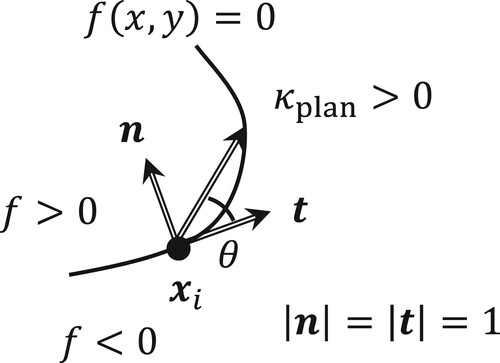
, respectively. In contrast to piecewise linear surface models, the following control point is determined irrespective of the mesh borders. As depicted in , considering two orthonormal vectors, namely, normal and tangent vectors, the positional relationship is represented by
and
. This representation is similar to a polar coordinate expression.
Figure 1. Positional relationships of the current and following control points, in addition to variables for advancement.
The step length is first adapted to confine the deviation from the exact (yet unknown) curve into a standard referred to as the tolerance, as denoted by Tolx. Considering the advancement from the current control point to the following point, let
and
denote the shift from the current control point and the tangent angle from
(unit tangent vector) to
, respectively. The shift vector is then expressed as follows:
(3)
(3) Denoting the current point by
, the elevation at point
is estimated using the Taylor expansion with respect to
as follows:
where
denotes the initial tangent angle. When
is determined and fixed,
is then adjusted to contain
within the tolerance. Angle
is updated based on the Taylor expansion of
as a function of
as follows:
To update
closer to 0,
should be set as follows:
(4)
(4) This process is repeated until
is contained in the standard. The difference of
impacted by the above is inspected until it is smaller than Tolx, which results in the following:
The elevation tolerance is then formulated as follows:
(5)
(5) Although the right-hand side enforces
, i.e.
, a safer constraint is applied as follows:
(6)
(6) If the sign of
changes during the iteration, there is a solution between two successive updates. Let
be the shift vector at the
th step. There is a solution if the following is true:
(7)
(7) In addition, there are constraints derived by (5) if the following is true:
(8)
(8) The update of
is then discontinued to proceed to the following control point.
3.2. Restriction and adaptation of the step length
Key restrictions for the step length are associated with the deviation of the exact curve. In addition to the piecewise arc approximation, the tangent angle is related to the step length
and plan curvature
as follows:
(9)
(9) Combined with Constraint (6),
should be restricted as follows:
(10)
(10) The tangent angle determined by Iteration (4) applied to the surface model includes the influence of the approximation. Given that the curvature
in (9) is a local quantity, the value of
obtained by (9) differs from that computed by Iteration (4) in addition to a finite value
. Thus, the step length
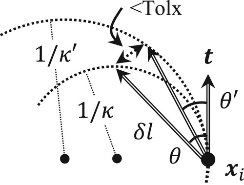
should be constrained by considering the approximation error. Let
be the plan curvature on
, and
be the tangent angle estimated by
. Based on , the distance between the two following points regulated by
and
is as follows:
(11)
(11) It should be noted that the Taylor expansions of
and
around
are respectively expressed as follows:
Figure 2. Difference between tangent angles estimated by two curvatures.
Moreover, Equation (11) is evaluated in the following form:
To incorporate this distance into a standard, i.e. Tolx, the step length
is constrained with respect to the following:
(12)
(12) During advancement, aversion to both understepping and overstepping is essential, for which
is constantly adjusted. To circumvent understepping, tracing acceleration is attempted as follows:
(13)
(13) In contrast, overstepping is averted with the maximum step length, which is denoted by
. The step length is then restricted as follows:
(14)
(14) Combining (12), (13), and (14), the step length is elongated and constrained based on the following:
(15)
(15) Once
is adjusted to follow (12),
is fixed and seeks
until (7) and (8) hold. If such an
cannot be determined within a certain number of iterations,
is then contracted to re-attempt determination by the following:
(16)
(16) Empirically, the constants
and
are set as 2 and 1/2, respectively.
Inspection of (4) implies potential divergence where , that is, the following point is inadvertently positioned around a stationary point. To circumvent the stall around such critical points, contraction based on (16) is applied. Although empirical, this is performed unless the following is true:
(17)
(17)
3.3. Identifying initial control points
To initiate tracking using the framework developed in the previous subsections, the determination of an initial point is required. This translates to identifying a solution, such that the following is true:
A straightforward method is to identify all solutions on the edges across the entire region, which is possible if the elevation function is a two-dimensional polynomial. Solutions on the edges perpendicular to the y-axis are obtained for a fixed constant y, and those on the x-axis are obtained for a fixed constant x. For the bicubic spline function (2), the first task is reduced to identifying the real roots of a cubic equation for x. Although analytical methods are available, a numerical method was adopted to achieve faster computation. Computing the eigenvalues of the companion matrices (Edelman and Murakami Citation1995) is a common technique. All real roots on both the horizontal and vertical edges of the entire mesh are obtained as candidate initial points.
One notable difference from piecewise linear tessellations is that only a single initial point is sufficient to identify a single contour object. This may render multiple remaining points redundant, and those on the same contour should be eliminated to circumvent duplicate detection. A technique based on piecewise arc approximation was considered in this study.
Another difference from piecewise linearity is the challenge associated with identifying complete sets of objects in the entire region. Although the majority of contours intersect with edges, there may be small-sized closures that do not intersect with any of the edges. These cannot be detected only with initial points on the original edges for which the disaggregation of a patch is necessary for the search for intersections.
3.4. Gleaning redundant initial points
When a single initial point is given, no other point on the same contour object is required, which is in contrast to piecewise linear tessellations. During single-step advancement, points proximal to the approximated arc are identified to eliminate from the list of candidate initial points. The concept of the overhang vector (Goto Citation2021), among others, is utilized to achieve this.
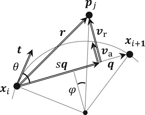
Let and
be two control endpoints. Consider an approximated arc and candidate initial point
, as shown in . Let
and
. The orthogonal projection of
onto
is
, where the following is true:
If
, the projection of
to segment
is on segment
. An overhang vector for
, as denoted by
, is introduced to quantify the distance from the segment as follows:
(18)
(18) The overhang of the approximated arc is obtained geometrically. Denoting this by
, it is quantified by the following:
(19)
(19) where
In the above,
is the unit tangent vector, and
.
Figure 3. Gleaning points proximal to an arc portion.
Let Tolh (Tolx) be the tolerance for the overhangs. Subsequently, the set of proximal points
that satisfies.
(20)
(20) is obtained to eliminate them from the list of initial points. Besides the inspection by the overhang, points proximal to endpoints are obtained in the case of
and
. They are identified by the following:
(21)
(21) The two tolerances, Tolx and Tolh, reflect the extent of the minimum computational resolution limit and the maximum error for piecewise arc approximation, respectively.
3.5. Termination or discontinuation
If the current control point approaches either the initial point or any of the borders of the analysis region, the step length may be adjusted to circumvent passing over the initial point or exceeding the border.
Let be the initial point. When the current step length is constrained by 3.1 follows:
whether or not the next point will potentially return to
, the step length is shortened according to
during preparation for potential closure. In conjunction with this adaptation, if the following point is identical to
, then a closed contour is detected, and the advancement is terminated.
Let and
be the region of analysis and distance from
to
, respectively. If the following is true:
is contracted by the following:
to avoid inadvertently exceeding the border. Further, if the following is true:
(22)
(22) the advancement is discontinued, assuming the control point reaches a border. The tracking is then reversed, and advancement is continued until the control point reaches another border. An open contour is detected.
3.6. Identifying small contours inside a patch
In the proposed algorithm, candidate initial points are searched for only at the edges of the original mesh. Small-sized closures remain undetected if they do not intersect with any of the edges. To identify small loci, for bicubic spline surface functions, and patch disaggregation is conducted for closer inspection. Given that the identification of a potential solution is intractable, the objective is to confirm non-existence, thus averting excessive disaggregation.
For simplicity, in this study, we investigated a square patch with dimensions of . This assumption does not lose generality. In conjunction with scaling, the same inspection is applicable to rectangular and/or disaggregated patches. Thereafter, EquationEq. (2
(2)
(2) ) can be re-written in matrix form as follows:
(23)
(23) where
and
. If there is no intersection at edges
and
, the following is true on
:
Hereafter, the inspection is limited to
because the same framework is applicable to the opposite case.
Given a fixed ,
is a cubic function with respect to
and has a maximum of two extremums. The locations of the potential extremums are the real roots of the quadratic equation:
(24)
(24) where
and
. If the real roots are in the range of
, the positiveness of the values on the points is checked. This is performed for the bottom and top borders, i.e.
. The formal representation is as follows:
(25)
(25) for
and real root(s) between
in (24). In an analogous manner, the same type of investigation is conducted for the left and right borders, where
. If any of the conditions do not hold, intersections exist such that
, and the patch is not disaggregated.
Further conditions for ensuring non-existence rely on a tangent surface on the borders. The tangent surface on a fixed is expressed as follows:
where
. If the elevation of this surface based on the left border at
is constantly above 0 on the opposite side, i.e.
, then the following is true:
(26)
(26) Conversely, considering the tangent surface on the opposite border at
, the elevation on the left border at
is expressed as follows:
(27)
(27) Similar to the investigation of
above, Conditions (26) and (27) for all
are checked. The left-hand sides are cubic polynomials with respect to
, for which the positiveness can be checked in a manner analogous to that for
. The corresponding derivatives with respect to
are those multiplied by
to replace
. For example, the stationary points on the left-hand side of EquationEq. (26
(26)
(26) ) are located at the roots of the following:
(28)
(28) The elevations are checked only if there are real roots in the range of
. In addition to the two conditions of
at
and
, if the following is true for
:
(29)
(29) and the real root(s) of (28) between
, the necessary conditions for non-existence are then satisfied.
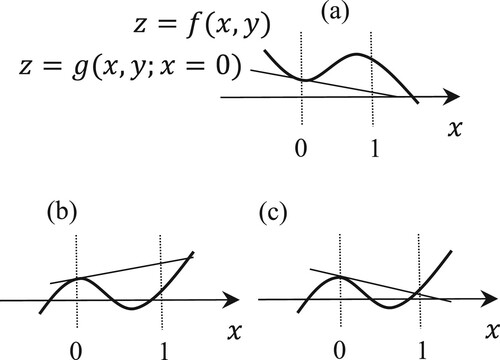
Only Conditions (25) and (29) do not guarantee non-existence. illustrates the three scenarios of tangent surfaces on the left border, where . Moreover,
and
are true for all cases, and Cases (b) and (c) have intersections at
in the range of
. Such cases occur when the tangent point is on a concave surface. To avert misidentification, another tangent surface on the opposite border, i.e. (27), should be verified:
does not hold, whereas
holds. All the inspections above are conducted for the left and right borders, that is,
, in addition to the bottom and top borders, that is,
.
Figure 4. Existence of cubic function roots.
If all conditions are not satisfied, the non-existence of a solution inside the patch is assured, and further disaggregation is discontinued. Otherwise, the current patch is disaggregated to search for potential closures. The simplest type of disaggregation was adopted in this study, where the square patch was disaggregated into four square patches divided by two borders, that is, . The same inspection is performed for each disaggregated patch. If an intersection
is found on the borders, further disaggregation is skipped. This is valid because the bicubic spline function in (23) cannot contain two closures inside the original patch. Thus, disaggregation is conducted recursively until the edge length contracts below the standard.
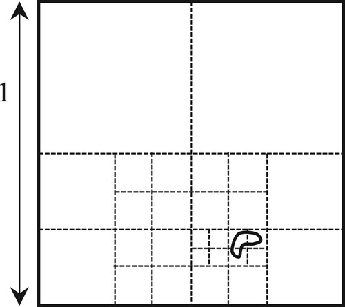
presents an example of the disaggregation of the original patch with dimensions of . As several positive conditions do not follow the outermost borders, the original patch is subdivided into four pieces. All conditions are then satisfied for the upper two patches, which ensures the non-existence of a solution, and no further disaggregation is conducted. In contrast, the lower two patches are disaggregated into four
-sized patches. With respect to the eight
-sized patches in the lower right, intersections are found on the edges, for which the recursive subdivision is discontinued, and the coordinates of the intersections are added as candidate initial points. If the non-existence conditions continue to be satisfied, the recursive process is repeated until the edge length is below the standard Tolp. A smaller tolerance may aid in the identification of small-sized contour objects, with an impact on the computation time.
Figure 5. A small closure detected by the recursive disaggregation of patches.
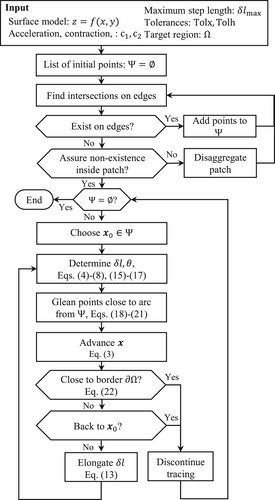
3.7. Entire flow
The individual components considered above were organized for enhanced visibility and accessibility. The flow of the proposed framework is outlined in . First, a surface model is determined using a digital elevation model dataset. The target elevation is subtracted to focus on solving
. Intersections on the borders of the patches are then identified as candidate initial points, which is exhaustively conducted. If non-existence in a target patch cannot be assured, it is disaggregated for further inspection. After identification, an initial point
is selected from the list of points
, which required no elaboration. The selection of the first point is sufficient. The tracking process is then initiated. It should be noted that step-length adaptation requires elaboration considering both the curvature error and tolerances. When the step length
is determined, the identified points in
that lie on the same contour are eliminated and canceled using as initial points. The control point
is advanced, which is repeated until it returns to the initial point
or encounters a boundary of the target region
. In each advancement, step length elongation is applied where and if possible.
Figure 6. Proposed algorithm for identifying complete sets of contour objects.
The procedures described above are used to detect and identify a complete set of contour objects for a single target elevation. Most practical outlets are accompanied by repetitive applications of this module for varying elevations, which are typically at a constant interval.
4. Demonstrative experiments
4.1. Study area
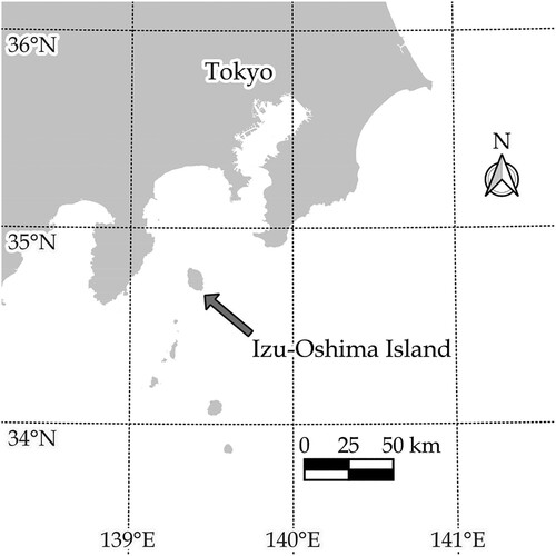
An isolated island located in the south of central Tokyo, Japan, was selected as the study area. The island is referred to as Izu-Oshima, and its location is shown in . It has an area of approximately 91.06 , and the average annual precipitation and temperature during 1991–2020 were 2858 mm and 16.4
, respectively. At the center of the island is an active volcano, namely, Mt. Miharayama, with an elevation at the summit of 764 m. A major eruption occurred in 1986, in addition to volcanic tremors and minor eruptions. There is a large caldera vent around the center along this line.
Figure 7. Location of Izu-Oshima island, Tokyo, Japan.
4.2. Experiment conditions
In this study, a digital elevation dataset was used, namely, ‘Digital Map 50 m Grid (Elevation)’, which was published by the Geospatial Information Authority of Japan. The mesh size was 2.25 s 1.5 s in the longitude and latitude directions, respectively, which corresponds to approximately 57.24 m
46.22 m. Although in recent years, higher resolution datasets, e.g. 0.4 s
0.4 s, have been made available, coarser resolutions were used to exploit the significance of the proposed framework. The elevation of the ocean was set as −1 m to estimate the coastline by searching for contours with elevations of h = 0 m. Contour detection was conducted for elevations varying from 0–750 m at intervals of 10 m or 25 m.
A personal computer (PC) equipped with an Intel® Core™ i7-1185G7, 3.00 GHz processor, and 32 GB of random access memory (RAM) running Windows 11 Professional was used. The associated program codes were implemented in MATLAB R2023a.
4.3. Contour detection
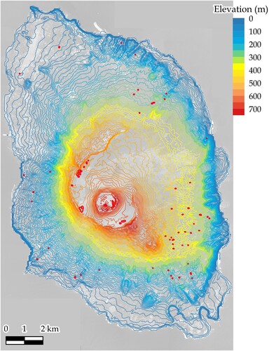
The cartographic contour extraction was performed in a straightforward manner. presents an overview of the outlet detected using the proposed framework, in which the contours were colored in varying gradations from blue to red. The elevation interval was 10 m. Several small contours were highlighted in red, thus indicating the presence of a depression inside the region. All extracted objects were oriented, for which convexity or concavity was assessable.
Figure 8. Contours identified using the proposed framework (Framework A).
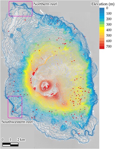
presents the outlet computed using the preceding algorithm developed in Goto and Shimakawa (Citation2016). The tracking algorithm considers the roundness of the curve, which is evaluated using three curvature-associated quantities. Although the smoothness of curves and storage efficiency are core advantages, the method to obtain initial points requires improvement, and the candidate points have been sought on a piecewise linear surface model. A direct comparison of and reveals a difference: a greater number of depression contours in red can be observed in . There are steep cliffs and jaggy coastlines around the northern and southwestern areas, as designated by magenta boxes. reveals small contours around the reefs, which are not present in .
Figure 9. Contours identified using the method established by Goto and Shimakawa (Goto and Shimakawa Citation2016) (Framework B).
To observe the significance of this application, four types of contour identification were tested: (A) the established framework, (B) a framework focusing on roundness developed by Goto and Shimakawa (Citation2016), (C) a piecewise triangular tessellation, and (D) a bilinear spline model. reports the profiles of the objects reproduced by the four frameworks with elevation intervals of 25 m, in addition to the experimental parameters. For the first two, namely (A) and (B), the number of independent polygons, duplicate detections, total number of control points, and average step length are reported. For the latter two frameworks, (C) and (D), all initial points were used to link each other, for which there were no redundant initial points.
Table 1. Contour profiles identified using the three frameworks.
A duplicate detection indicates that the identified contour object was already detected and listed by a preceding process initiated from a different initial point. This was deemed true if the area, perimeter, and centroid of an identified object were all close within a threshold to an entry in the list of independent objects. Along with this standard, Framework (B) encountered frequent duplications in various elevations, while the proposed framework (A) did not exhibit such inefficiency. This enhancement was achieved by piecewise arc approximation between successive control points, along with the elimination technique of initial points established in Section 3.4. Although duplicate detection might occur with different parameters – for instance, tighter tolerances Tolx and Tolh – the current configuration was able to avert it.
It should be noted that the number of objects identified by (A) was greater than that identified by (B) at most elevations. For example, with respect to an elevation of h = 0, Framework (A) detected 67 independent contours, whereas only two were detected using Framework (B). The main difference was the small contours distributed around the northern and western shores. At an elevation of h = 750 m, Framework (A) detected one small contour, whereas (B) did not. This is because of the non-existence of an intersection in the piecewise linear surface for Framework (C), whereas Framework (B) was dependent on identifying the initial points. Although the maximum step length was set as the same value for Frameworks (A) and (B), the average step length in Framework (A) was half of that in Framework (B). Consequently, this enhanced the identification of the other initial points along the trajectory. For Frameworks (C) and (D), the step length was restricted by the sizes of the triangular and rectangular patches. The length of the former was slightly smaller than half of the longer edge length, while the length of the latter was slightly smaller than the shorter edge length.
To inspect the computational efficiency in Framework (A), the computation times were measured for varying tolerance for patch disaggregation, namely Tolp. The times were measured by the ‘cputime’ function, with which the resulting time may fluctuate by each trial depending on the CPU load. reports the computation times in seconds consumed by three parts: (1) finding initial points on the original mesh, (2) those on disaggregated patches, and (3) contour tracking initiated from a detected initial point. The depth of disaggregation indicates the maximum number of recursions to find the root(s) or confirm non-existence. The elapsed times for finding initial points on the original mesh were shorter than 1 min in all cases, while those for contour tracking, including gleaning of redundant initial points, were approximately 20 s. By contrast, the consumed times to find initial points on disaggregated patches were shorter than 2 s, even with the smallest Tolp = 0.001 m. The number of detected contours was 264, with the largest Tolp = 10 m, while those with smaller ones were all 266: two small contours were detected with Tolp 1 m. Even with a small Tolp, the computation time in total would not increase significantly, and the target precision should rather be determined by the resolution of the dataset. Considering the mesh size, Tolp = 1 m may suffice in this experiment.
Table 2. Computation times with varying tolerances for patch disaggregation.
A further comparison of the four frameworks was conducted. and present the magnified outlets by the four frameworks focused on the northern and western reefs demarcated in with elevation intervals of 25 m. The red contours reflect the depression inside each object. In , the runway of Oshima Airport is visible in the lower left, where no contour was identified. From a detailed inspection of Frameworks (A) and (B), it can be seen that both exhibited smooth curves, and only the former detected several small objects in the northern reef of the coastline. To compare the proposed framework with traditional frameworks, oriented contour tracking algorithms were applied to piecewise triangular and bilinear spline surface models in Frameworks (C) and (D), respectively. In contrast to the bicubic spline model, red objects indicating depressions emerged in the lower part, which would relate to the approximation error inevitable in lower-order surface models. Further, a close inspection of Framework (C) reveals a notable modeling error on the headland in the west northernmost. While only one narrow hill was detected in Frameworks (A), (B), and (D), it is inadvertently separated into two hills in Framework (C) due to the ambiguity specific to piecewise triangular modeling.
Figure 10. Identified contours around the northern reef using the four methods.
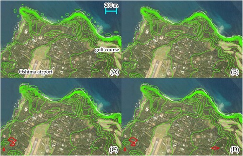
Figure 11. Identified contours around the southwestern reef using the four methods.
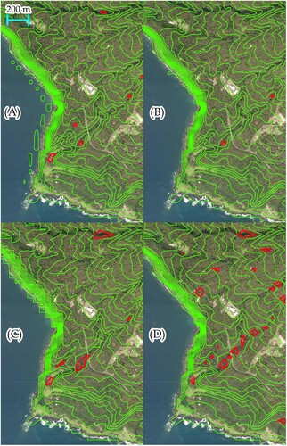
A comparison of Frameworks (A) and (B), as shown in , reveals a trend similar to that in . Framework (A) could identify small objects along the western coastline compared with Framework (B), and Framework (C) reproduced jagged coastlines compared with the other ones. In Framework (D), a larger number of red objects were detected along a gutter toward the southwest, yet it would be deemed an approximation error because the elevation would decrease in a monotonic manner along a runoff or stream. In fact, most contours around the gutter are receded and not closed in Frameworks (A) and (B).
4.4. Three-dimensional consistent contour-based network
Another application of the proposed framework was tested. A three-dimensional manipulation framework for a bicubic spline surface model established in Goto (Citation2021) was applied. It should be noted that streamlined tracing along the steepest upward and downward directions aids in reproducing a three-dimensionally consistent contour-based network (3D-CBN). The framework proposed in this study was used as an external module. presents an overview of the outlook of the 3D-CBN, whereas presents a magnification of the cliffs in the north and the scoria cone in the south, as demarcated in . Frameworks (A) and (B) were assessed for comparison, and the outlets are delineated with elevation intervals of 10 and 25 m in the northern and southern outlets, respectively. The green objects indicate contours identified by the proposed framework, whereas cyan and magenta objects indicate the steepest upward and downward streamlines, respectively. In the upper CBNs, two major steep hills were observed in the left and right parts close to the coastline, whereas the upward streamlines converged to local maxima without oscillation. Streamline tracing is continued until it either encounters a stationary point or reaches the lower or upper limit of the elevation interval. Upon reaching such a limit, the tracing discontinues to evaluate if multiple streamlines are proximal or confluent. This may ensue that, if the contour detection is not complete, tracing may terminate inadvertently. In the upper outlet by Framework (B), such a flaw was observed in the right part demarcated by the yellow frame. By contrast, the reproduced CBN by Framework (A) is complete and consistent topologically.
Figure 12. Overview of the three-dimensionally consistent contour-based network.
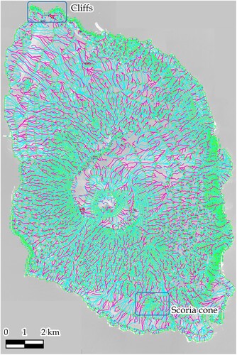
Figure 13. Detailed contour-based network around the cliffs and scoria cone.

In the lower outlets of the scoria cone, the green contours are roundish, from which the steepest upward streamlines moved toward the top of the hill. There seemed little difference between Frameworks (A) and (B) in this area. It should be noted that the mesh size was approximately the quarter length of the scalebar, and the peak location of the cone could be identified in a precise manner in conjunction with the underlaid aerial photo. A driving school was observed at the top, and no contour was detected around it. This may indicate that the premises are built on a flat area.
4.5. Slope analysis
The proposed framework was utilized for further application to slope analysis. Given a continuous elevation function of , the slope was quantified by the magnitude of the gradient vector, i.e.
. The interpolated values of
on a regular rectangular lattice were provided as elevation values.
delineates the outlet of the slope analysis with a color gradation from green to red, in which the isovalues varied in intervals of 0.1. The values of = 0.1, 0.5, and 1.0 correspond to approximately 5.7, 26.6, and 45.0 degrees, respectively. Red objects emanated around the northern, western, and eastern coastlines. The two regions in the northern cliffs and the scoria cone were magnified for closer inspection, and Frameworks (A) and (B) were again assessed for comparison. The cyan curves in correspond to geographical contours with an elevation interval of 25 m. The solid and dashed curves indicate that the values inside the curve are greater, i.e. steeper (respectively smaller and less steep) than those on the contour.
Figure 14. Overview of the island based on the slope analysis.
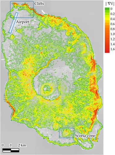
Figure 15. Detailed slope analysis around the cliffs and scoria cone.
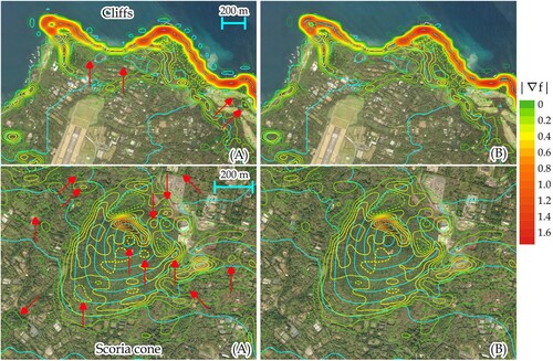
Along the northern coastline, the red curves existed, which exhibit the steepness of the cliffs. While relative steepness might be assessed by observing the density of contours, the outlet delineated in can quantitatively detail the extent. In view of the upper two outlets, successive closures on the left side of the runway signify that the shape of the hill is acute. In contrast, dashed contours were observed to the west of the golf course, for which the slope turned gentle toward the ridge. While Frameworks (A) and (B) might have reproduced similar outlets, there were differences in the ability to detect small closures: the green and light green contours detected by Framework (A) designated by red arrows did not exist in the outlet by Framework (B).
In the lower two results of the scoria cone, the cyan curves indicate again elevations at intervals of 25 m. The height of the cone is thus some 150 m from the base. Approximately 100 m north of the top of the hill, there was a series of solid brown contours, which implies the existence of a locally steep slope. The yellow ‘8’-shaped dashed contour located south of the hilltop indicates the slope is gentler than the surrounding locations. Along these lines, a series of solid objects implies that the surface is acute, whereas those of the dashed lines imply that the slope turns gentle toward the inside. The ability to detect small closures by Framework (A) was significant in the lower outlets. The green and light green closures designated by red arrows were not detected by Framework (B). It is worth noting that Framework (B) relies on piecewise triangular tessellation to find candidate initial points, in which greater approximation errors might be contained in the surface model. The slope measure includes differentiations of the elevation function
, for which it would vary more sharply than the elevation itself. While isolines for this type of quantity would contain many small closures, the established Framework (A) provided a complete detection scheme suited for bicubic spline models.
The outlet comprises a set of signed polygons and not a raster image. Current popular analyses using geographic information system (GIS) functionality are inextricably related to raster analysis, for which the outlet turned jagged when magnified. In contrast, by utilizing the proposed framework, the method of slope analysis was transferred to vector- or polygon-based; the overlay of other vector-based objects, including geographical contours, would evolve analytical techniques to exploit better insight: an additional option for delineation is gained.
5. Conclusions
The core objective of contour detection is to identify loci such that
. Piecewise linear tessellation provides a straightforward solution to the resulting commodity in GIS-based analyses. All intercepts are determined and used as control points that connect two neighboring points. Its structural simplicity simplifies the calculation and delineation objectives, thus yielding byproducts of jagged outlets when magnified. In contrast, bicubic spline tessellation presents a challenge with respect to both theoretical and computational aspects. In addition to the non-linearity of the elevation function, the number of independent trajectories on and in a unit patch is yet to be determined.
Given a fixed constant x or y, interceptions can be computed by solving a cubic polynomial. A preliminary tracking method on bicubic spline surfaces was established in Goto and Shimakawa (Citation2016), in addition to a detailed formalization of curvature-associated quantities. It is yet to be determined which interceptions should be used as initial points to identify independent objects, thus averting duplicate detection if possible.
Significant achievements made in this study include the complete detection of candidate initial points and the elimination of those lying on the same contour object. Mathematically, the former problem is intractable when confirming the existence of a solution on or inside a region. In this study, a computational inspection method for verifying the non-existence of a solution was developed. In particular, if non-existence cannot be ensured in a current region, it is subdivided into four portions, which are inspected recursively. Tolerance is essential to circumvent excessive disaggregation significantly below the precision of the original dataset.
The elimination of the initial points on the same contour curve is dependent on the buffered elimination along the approximated arc portion. To attain a higher elimination rate, a slight adjustment of the step length is necessary, and excessive contraction results in computational and storage inefficiencies, whereas improper elongation fails to eliminate the initial points. Tolerance is critical in this procedure. In particular, for the comparison of local curvatures at two distinct points, the step length is adapted to contain the error by piecewise arc approximation into the standard, i.e. tolerance. With the exhaustive detection of the initial points, this method is invaluable for the improved prevention of the redundant detection of identical objects. The experimental results in provide a practical benefit: no duplicate detection of the same object was observed.
The evolution of contour detection for bicubic spline surfaces, particularly concerning the completeness of identified objects, provides new possibilities for numerous applications to GIS-based analyses in various fields, namely, engineering, geography, and earth science. The two demonstrative examples address applications for generating 3D-CBN and slope analysis. The former experiment exhibited significant affinity with streamline tracking: the smoothness of the identified curves was significant, and the location identification of ridges and local peaks was well-demonstrated.
The other application to slope analysis provided richer possibilities and insightful outlets, particularly via detailed delineations. In contrast to the current slope analyses, which are inextricably related to raster-based assessment, the fundamental method of analysis has transitioned to vector-based assessment. In addition to quantifying the extent of steepness and identifying the tracking direction, the detected object is accompanied by the orientation of the closure. The sign of a closed object provides a measure of whether the slope inside the object is greater or smaller. Inside the contours with negative and smallest absolute values, the terrain around the region may be considered almost flat. Although the steepness may be assessed upon observing the density of geographical contour curves, this is unsuitable for quantitative assessments. To date, slope analysis has been employed for this objective; however, a typical or averaged value is associated with a single patch, for which detailed analysis was ruled out, where only previous or coarse datasets are available. The final experiment demonstrated a promising application that was addressed and implemented in raster-based analysis contexts.
The proposed framework was developed on a mathematical basis, for which the completeness of object detection, including small-sized closures, was achieved. Moreover, storage and computational efficiencies were minimized when compared with the framework proposed in Goto and Shimakawa (Citation2016). This is a byproduct of completeness, and further advancements with regard to inspecting the non-existence or existence of a solution on or inside a rectangular region will be conducted in future research.
Disclosure statement
No potential conflict of interest was reported by the author(s).
This research was funded by the JSPS KAKENHI Grant Number 21K01021.
Data availability statement
The datasets that support the findings of this study are openly available in ‘Mendeley Data' at http://dx.doi.org/10.17632/f4hfsfrsy4.1. All of them are preserved in the ESRI’s Shapefile format.
Additional information
Funding
References
- Andújar, Carlos, Pere Brunet, Antoni Chica, Isabel Navazo, Jarek Rossignac, and Àlvar Vinacua. 2005. “Optimizing the Topological and Combinatorial Complexity of Isosurfaces.” Computer-Aided Design 37 (8): 847–857. doi:10.1016/j.cad.2004.09.013.
- Edelman, Alan, and Hiroshi Murakami. 1995. “Polynomial Roots From Companion Matrix Eigenvalues.” Mathematics of Computation 64: 763–776. doi:10.1090/S0025-5718-1995-1262279-2.
- Evans, I. S. 1972. “General Geomorphometry, Derivatives of Altitude, and Descriptive Statistics.” In Spatial Analysis in Geomorphology, edited by R. J. Chorley, 17–90. London: Harper & Row.
- Garfias Royo, Margarita, Priti Parikh, and Jyoti Belur. 2020. “Using Heat Maps to Identify Areas Prone to Violence Against Women in the Public Sphere.” Crime Science 9 (article number 15): 1–15. doi:10.1186/s40163-020-00125-6.
- Gong, Xin-Yi, De Xu Hu Su, Zheng-Tao Zhang, Fei Shen, and Hua-Bin Yang. 2018. “An Overview of Contour Detection Approaches.” International Journal of Automation and Computing 15 (6): 656–672. doi:10.1007/s11633-018-1117-z.
- Goto, Hiroyuki. 2021. “Three-dimensionally Consistent Contour-Based Network Rendered From Digital Terrain Model Data.” Geomorphology 395: 107969. doi:10.1016/j.geomorph.2021.107969.
- Goto, Hiroyuki, and Yoichi Shimakawa. 2013. “Lightweight Calculation of the Area of a Closed Contour by an Inner Skin Algorithm.” Journal of Computations and Modelling 3 (1): 57–77.
- Goto, Hiroyuki, and Yoichi Shimakawa. 2016. “Storage-Efficient Method for Generating Contours Focusing on Roundness.” International Journal of Geographical Information Science 30 (2): 200–220. doi:10.1080/13658816.2015.1080830.
- Goto, Hiroyuki, and Yoichi Shimakawa. 2017. “Storage-Efficient Reconstruction Framework for Planar Contours.” Geo-spatial Information Science 20 (1): 14–28. doi:10.1080/10095020.2016.1194603.
- Guan, Y. Q., Y. Y. Cai, Y. T. Lee, and M. Opas. 2006. “An Automatic Method for Identifying Appropriate Gradient Magnitude for 3D Boundary Detection of Confocal Image Stacks.” Journal of Microscopy 223 (1): 66–72. doi:10.1111/j.1365-2818.2006.01600.x.
- Haijun, Liu, and Yi Yongping. 2010. “Application of Contour Map Creating Technique in Magnetic Exploration.” Paper presented at the 3rd International Conference on Computer and Electrical Engineering, Chengdu, November 16–18.
- Hanyan, Huang, Shao Mingshan, Zhang Hua, and Chen Yulan. 2016. “Analysis and Visualization of Electromagnetic Situation Based on Raster Database.” Paper presented at the 2016 International Conference on Modeling, Simulation and Optimization Technologies and Applications, December 18–19.
- Henry, D., and H. Aubert. 2019. “Isolines in 3D Radar Images for Remote Sensing Applications.” Paper presented at the 16th European Radar Conference, October 2–4.
- Jang, Sukwon, and Hyochoong Bang. 2017. “Acquisition Method for Terrain Referenced Navigation Using Terrain Contour Intersections.” IET Radar, Sonar & Navigation 11 (9): 1444–1450. doi:10.1049/iet-rsn.2017.0023.
- Karim, Abdul, Samsul Ariffin, Azizan Saaban, and Van Thien Nguyen. 2021. “Construction of C1 Rational Bi-Quartic Spline With Positivity-Preserving Interpolation: Numerical Results and Analysis.” Frontiers in Physics 9: 555517. doi:10.3389/fphy.2021.555517.
- Krcho, J., and I. Haverlík. 1973. “Morphometric Analysis of Relief on the Basis of Geometric Aspect of Field Theory.” Acta Geographica Universitatis Comenianae, Geographico-Physica 1: 7–233.
- Li, Lu, Hu Peng, Xun Chen, Juan Cheng, and Dayong Gao. 2016. “Visualization of Boundaries in Volumetric Data Sets Through a What Material You Pick Is What Boundary You See Approach.” Computer Methods and Programs in Biomedicine 126: 76–88. doi:10.1016/j.cmpb.2015.11.014.
- Lihua, Tang, Xu Ai-jun, and Fang Lu-ming. 2008. “The Algorithm of Creating Contour Lines Based on DEM.” Paper Presented at the Proceedings of the Society of Photo-Optical Instrumentation Engineer, Guangzhou, November 11.
- Liu, Jintao, Xi Chen, Xingnan Zhang, and Kyle D. Hoagland. 2012. “Grid Digital Elevation Model Based Algorithms for Determination of Hillslope Width Functions Through Flow Distance Transforms.” Water Resources Research 48 (4): W04532. doi:10.1029/2011WR011395.
- Malamos, Nikolaos, and Demetris Koutsoyiannis. 2016. “Bilinear Surface Smoothing for Spatial Interpolation with Optional Incorporation of an Explanatory Variable. Part 2: Application to Synthesized and Rainfall Data.” Hydrological Sciences Journal 61 (3): 527–540. doi:10.1080/02626667.2015.1080826.
- Maple, C. 2003. “Geometric Design and Space Planning Using the Marching Squares and Marching Cube Algorithms.” Paper presented at the 2003 International Conference on Geometric Modeling and Graphics, July 16–18.
- Martínez-Frutos, Jesús, and David Herrero-Pérez. 2017. “GPU Acceleration for Evolutionary Topology Optimization of Continuum Structures Using Isosurfaces.” Computers & Structures 182: 119–136. doi:10.1016/j.compstruc.2016.10.018.
- Matuschek, Olaf, and Andreas Matzarakis. 2011. “A Mapping Tool for Climatological Applications.” Meteorological Applications 18 (2): 230–237. doi:10.1002/met.233.
- Maunder, Chris J. 1999. “An Automated Method for Constructing Contour-Based Digital Elevation Models.” Water Resources Research 35 (12): 3931–3940. doi:10.1029/1999wr900166.
- Mino, Lukáš, Imrich Szabó, and Csaba Török. 2016. “Bicubic Splines and Biquartic Polynomials.” Open Computer Science 6 (1): 1–7. doi:10.1515/comp-2016-0001.
- Neto, J. F. de Queiroz, E. M. D. Santos, and C. A. Vidal. 2016. “MSKDE – Using Marching Squares to Quickly Make High Quality Crime Hotspot Maps.” Paper presented at the 29th SIBGRAPI Conference on Graphics, Patterns and Images, São Paulo, October 4–7.
- Oka, Shriram, Akash Garg, and Koshy Varghese. 2012. “Vectorization of Contour Lines from Scanned Topographic Maps.” Automation in Construction 22: 192–202. doi:10.1016/j.autcon.2011.06.017.
- O'Loughlin, E. M., D. L. Short, and W. R. Dawes. 1989. “Modelling the Hydrological Response of Catchments to Land Use Change.” In Proceedings of the Hydrology and Water Resources Symposium, 335–340. Canberra, Australia.
- Parsian, Saeid, Meisam Amani, Armin Moghimi, Arsalan Ghorbanian, and Sahel Mahdavi. 2021. “Flood Hazard Mapping Using Fuzzy Logic, Analytical Hierarchy Process, and Multi-Source Geospatial Datasets.” Remote Sensing 13 (23): 4761. doi:10.3390/rs13234761
- Popowicz, A., and B. Smolka. 2014. “Isoline Based Image Colorization.” Paper Presented at the UKSim-AMSS 16th International Conference on Computer Modelling and Simulation, March 26–28.
- Qiao, Weifeng, Yahua Wang, Qingqing Ji, Yi Hu, Dazhuan Ge, and Min Cao. 2019. “Analysis of the Evolution of Urban Three-Dimensional Morphology: The Case of Nanjing City, China.” Journal of Maps 15 (1): 30–38. doi:10.1080/17445647.2019.1568922.
- Rui, Xiao-ping, Xianfeng Song, and Yi-wen Ju. 2010. “An Isoline Rendering Method Considering of Constrained Conditions.” 2010 IEEE International Geoscience and Remote Sensing Symposium, 4007–4010.
- Rui, Xiao-ping, Xianfeng Song, Yongguo Yang, and Yi-wen Ju. 2011. “An Improved Method of Rendering oil Extraction Contour Under Constrained Conditions.” Mining Science and Technology (China) 21 (3): 337–342. doi:10.1016/j.mstc.2011.05.007
- Rulli, M. Cristina. 2010. “A Physically Based Watershed Partitioning Method.” Advances in Water Resources 33 (10): 1206–1215. doi:10.1016/j.advwatres.2010.06.011.
- Schneider, Bernhard. 2005. “Extraction of Hierarchical Surface Networks From Bilinear Surface Patches.” Geographical Analysis 37 (2): 244–263. doi:10.1111/j.1538-4632.2005.00638.x.
- Shangguan, M., M. Bender, M. Ramatschi, G. Dick, J. Wickert, A. Raabe, and R. Galas. 2013. “GPS Tomography: Validation of Reconstructed 3-D Humidity Fields with Radiosonde Profiles.” Annales Geophysicae 31 (9): 1491–1505. doi:10.5194/angeo-31-1491-2013.
- Shary, Peter A., Larisa S. Sharaya, and Andrew V. Mitusov. 2002. “Fundamental Quantitative Methods of Land Surface Analysis.” Geoderma 107 (1): 1–32. doi:10.1016/S0016-7061(01)00136-7.
- Song, Zhiyong, Liping Wang, Wenjian Tao, Qingzhao Li, and Wei Wang. 2016. “Research on the Mechanism of Curvature About Complex Surface Based on Five-Axis Flank Milling.” Procedia CIRP 56: 551–555. doi:10.1016/j.procir.2016.10.108.
- Tadini, A., N. Azzaoui, O. Roche, P. Samaniego, B. Bernard, A. Bevilacqua, S. Hidalgo, A. Guillin, and M. Gouhier. 2022. “Tephra Fallout Probabilistic Hazard Maps for Cotopaxi and Guagua Pichincha Volcanoes (Ecuador) With Uncertainty Quantification.” Journal of Geophysical Research: Solid Earth 127 (2): e2021JB022780. doi:10.1029/2021JB022780.
- Tan, Liheng, Gang Wan, Feng Li, Xiaohui Chen, and Wen-long Du. 2017. “GPU Based Contouring Method on Grid DEM Data.” Computers & Geosciences 105: 129–138. doi:10.1016/j.cageo.2017.05.007
- Vannier, E., R. Dusséaux, O. Taconet, and F. Darboux. 2019. “Wavelet-Based Clod Segmentation on Digital Elevation Models of a Soil Surface With or Without Furrows.” Geoderma 356: 113933. doi:10.1016/j.geoderma.2019.113933.
- Victoria, Mariano, Pascual Martí, and Osvaldo M. Querin. 2009. “Topology Design of Two-Dimensional Continuum Structures Using Isolines.” Computers & Structures 87 (1): 101–109. doi:10.1016/j.compstruc.2008.08.001.
- Xu, Bin, Jianping Chen, and Meijuan Yao. 2016. “Identification of Contour Lines From Average-Quality Scanned Topographic Maps.” Mathematical Problems in Engineering 2016: 1–14. doi:10.1155/2016/3089690.
- Yang, Fan, and Zhenghong Dong. 2020. “Research on Electromagnetic Visualization Method.” International Journal of Modeling, Simulation, and Scientific Computing 11 (05): 1–11. doi:10.1142/s1793962320500373.
- Zhou, Chen, and Manchun Li. 2021. “A Systematic Parallel Strategy for Generating Contours From Large-Scale DEM Data Using Collaborative CPUs and GPUs.” Cartography and Geographic Information Science 48: 187–209. doi:10.1080/15230406.2020.1854862.