The fractal or scaling perspective on progressively generated intra-urban clusters from street junctions

ABSTRACT

The underlying complexity of urban space can be manifested by its fractal forms and scaling statistics. This paper examines these characteristics at the intra-urban scale through the lens of clustered street junctions (including road ends) in two Chinese metropolitan areas: Beijing and Shenzhen. We derived the cluster sets with Euclidean distance thresholds starting at 100 meters (m) and ending at 1000 m, and outlined each cluster using a concave-hull method to maintain their original irregular shapes. Within each delimited cluster, we examined four urban attributes: gross domestic product, number of street nodes, polygon area, and population. Our analysis revealed that power law distribution applied to almost every cluster set in terms of the four attributes, but varied from one attribute to another or from city to city, represented primarily by fluctuated power law exponents and ht-index values whose profiles along with the cluster growth can effectively characterize the urban structure. Additionally, we computed the spectrum of intra-urban scaling exponents with cluster size increments, contributing new insights into the allometric relationships between urban configuration and function.

KEYWORDS:

• Spatial clustering
• urban structure
• urban function
• power law
• intra-urban scaling law

1. Introduction

Traditional urban science has built a solid theoretical foundation that helps us understand complex urban system regarding their morphological aspects (such as central place theory; Christaller 1933; Chen 2011) and statistical aspects (for example, size distribution; Zipf 1949; Krugman 1996; Batty et al. 2008). In recent decades, fractal geometry and the thinking behind it have grown as a new paradigm of both aspects of urban studies (Batty and Longley 1997, Makse et al. 1998). The core concept of fractal geometry ‘self-similarity’ (Mandelbrot 1967), referring to a part of a fractal is similar to the whole, can be well-adopted as a good angle for us to investigate the urban space across different spatial scales (Shreevastava, Rao, and McGrath 2019). For instance, a city can be deemed as the concentration of human settlements or activities at the country scale. As Jacobs (1961) noted, a city needs a sufficient number of concentrations of people, so it is natural for a city’s surface to be filled with elements or artifacts of varying densities in the course of urban development. In most cases, a highly developed city is composed of a majority of low-density areas and a minority of high-density ones (clustered areas), just as a country is normally constituted by a majority of rural areas and a minority of urban areas. In this connection, it is plausible to cascade the country–city relationship inside a city for studying its high/low-density areas (Ma et al. 2020, 2021).

Spatial clustering is the most effective means of discovering the concentration at multiple levels of urban space, as each cluster is regarded as the concentration of city elements in which its members are at a closer distance or reminiscent of attributes than the non-member ones that reside outside. The most prominent example within the urban studies literature is the city clustering algorithm that joins adjacent raster cells using population density thresholds and achieved city boundaries beyond administrative definitions (e.g. Rozenfeld et al. 2008; Arcaute et al. 2015). For vector data, the agglomeration of individual locations can be done in a step-by-step manner. We can construct mathematical models for the relationship between number of clusters and clustering distance and thereby find the cutoff through locating the characteristic point on the fitted curve with maximum inflection (e.g. Tannier et al. 2011; Tannier and Thomas 2013; Masucci et al. 2015). With the development of geospatial big data, Jiang and colleagues coined the term ‘natural city’ (NC), which leveraged different types of location-based social media data to delimit city boundaries at country and global scales using a cutoff that guides the clustering process and is determined objectively by long-tailed statistics underlying the adjacencies between geotagged web content (e.g. Jiang and Jia 2011; Jiang and Miao 2015; Ma, Sandberg, and Jiang 2017).

A common feature of the above-mentioned methods is that scaling properties or power law statistics are found in detected clusters; that is, the imbalanced ratio between large-to-small cluster sizes (Long et al. 2018; Alvioli 2020; Montero, Tannier, and Thomas 2021). This echoes Goodchild’s (2004) note that there is no average place on the Earth’s surface. It is difficult to analyze such an imbalance ratio using a well-defined mean, as the statistical distribution of all cluster sizes is distant from a normal-like distribution and is very likely to be right-skewed as a power law that bears no characteristic scale. Thus, the measurement through a fixed length or size for the entire cluster set becomes ineffective, similar to using the length or area of a single trunk or branch to measure a whole tree. To effectively conduct the measurement, the term ‘scaling’ can be considered equivalently with ‘fractal’, according to the observation that whether or not there exist repeatedly disproportional ratios of small-to-large clusters within the entire data set and its sub-wholes, recognized as a self-similar relationship in a statistical manner (Jiang and Yin 2014). The number of recurring times of the imbalanced ratio – that is, the ht-index (see Section 2.3 for more details) – together with power-law-related metrics, can then help quantify the fractality of all clusters as a whole. Apart from the scaling pattern or the power law distribution of a single urban quantity, numerous studies also found the allometric relationship between population and other urban morphological, functional quantities (e.g. Naroll and Von 1973; Chen, Wang, and Li 2019; Lan, Li, and Zhang 2019). Urban allometry is closely tied to fractal dimension (West, Brown, and Enquist 1997; Batty and Longley 1997; Batty et al. 2008), and has become the fundamental urban theory – urban scaling law – developed by Bettencourt and his team (2007, 2010, 2013) indicating the super- and sub-linear relationships between urban population versus a set of urban measures such as innovations, gross domestic product (GDP), and infrastructures. So far, however, such a scaling or fractal perspective on both single and a pair of urban variables have rarely been taken together for the identification and quantification of intra-urban clusters that are used as the modeling units to infer the relationship between urban form and function for an individual city.

The present paper probes into the urban complex spatial structure and its relation to urban performance. Presumably, the spatial configuration of a city can be conceived as the emergence of scaling or fractal that evolves upon a growth view on the progressive formation of intra-urban clusters by slightly increasing Euclidean distance thresholds (straight-line distance between two points). We tend to believe that these clustering results, as well as their fractal or scaling properties, can substantially reflect the essence of the urban space. Rooted in fractal-geometric thinking, the study will not identify an optimal clustering cutoff or characteristic scale for effectively delimiting the boundary of a city or its centers, but will formulate a more holistic or systematic understanding on the spatial process of urban form through aggregating urban street junctions in a step-by-step fashion. The present study made three main contributions. Firstly, we clustered hundreds of thousands street junctions in a progressive way in Beijing and Shenzhen and leveraged concave-hull-based approach to delimit the border of each cluster that follows point spatial distribution and is fractal-like, leading to bottom-up, novel modeling units for the scaling analysis. Secondly, we found that the power law distribution of urban physical and socio-economic attributes within the intra-urban clusters always exists using clustering distance thresholds from 100 to 1000 m, but the degree of being a power-law differs in their exponents and the ht-index, inferring a monocentric or polycentric urban structure. Thirdly, we characterized the allometric relationship based on four within-cluster attributes in both cities and the spectrum of derived scaling exponents upon the cluster growth for each individual city can foster a better understanding of urban structure and its functioning with urban residents.

The remainder of this paper is organized as follows. Section 2 introduces the data sets and the designed methods for intra-urban clusters and related scaling analyses. Section 3 presents the results of the derived clusters between two mega cities in China, as well as the detailed change of scaling metrics of cluster size and pertained attributes with a series of clustering distance threshold. Section 4 further discusses the implication of the study. Section 5 concludes the study and points to future research directions.

2. Data and methods

2.1. Data and data processing

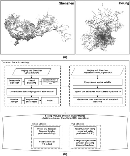
We selected two metropolises that belong to the top-tier cities in China: Beijing and Shenzhen. Both cities have a highly developed street structure that fully covers the urban area (Figure 1(a)). Two kinds of data sets are mainly utilized in this study: (1) city-level street networks, and (2) raster-based population and GDP data. The street network data were downloaded directly from OpenStreetMap (Bennett 2010) and are available at http://download.geofabrik.de/asia/china.html. We then relied on a developed ArcGIS toolbox (Ren 2018) to get street nodes that meet the criteria that a node must intersect with three segments or if they are dangling ends. There were 151,511 junctions in Beijing and 47,957 junctions in Shenzhen. For urban functional attributes, the population grid data was collected from Constrained Individual Countries 2020 United Nations (UN) adjusted Population Counts (http://worldpop.org) and has 100 m spatial resolution. The population data were based on buildings or residential areas from remote sensing and calibrated by UN population estimates 2019 to ensure their accuracy (Stevens et al. 2015). The GDP grid data for 2019 was first collected from the Resource and Environmental Science Data Center of the Chinese Academy of Sciences (http://www.resdc.cn/) at a spatial resolution of 1 km. As the time between gridded GDP and population data was inconsistent, we reassigned the GDP value in each grid according to the 2020 GDP statistics from the Chinese National Bureau of Statistics (http://www.stats.gov.cn/tjsj/ndsj/) by using the proportion of grided GDP values at 2019. The overall framework is described as per the flowchart in Figure 1(b). First, we clipped out both vector and raster data using administrative boundaries of Beijing and Shenzhen, then conducted zonal statistics of cells with GDP and population attributes for each city, which were further joined with intra-urban clusters.

Figure 1. (Color online) The street network data in Beijing and Shenzhen (a) and the methodological framework of this study (b).

2.2. Urban cluster detection and boundary delimitation

The study adopts an iterative clustering method for detecting individual urban concentrations from street nodes. Figure 2(a–d) uses Koch snowflakes at the first four levels to illustrate how the clustering algorithm works. According to the rule that a Koch snowflake unfolds, the length of a snowflake segment starts with one unit, then decreases at a ratio of one-third. For Koch snowflake at each of four levels, we start with any point of the snowflake and the corresponding segment length (1, 1/3, 1/9, 1/27) as the radius to draw a circle, and continuously use each of the other points within the circle as the circle center for the next step until all candidate points are traversed. A cluster is then formed by the points within those depicted circles whose radii are taken as the distance threshold. In this way, we can detect a point cluster by means of point–point proximity.

Figure 2. (Color online) The demonstration of the clustering algorithm applied on four-level Koch snowflake vertices, respectively, and the concave polygon of the clustered points. (Note: The gray points in Panels a–d are points are non-snowflake points and outside the circles with the search radius, so none of them can be included as the cluster member.)

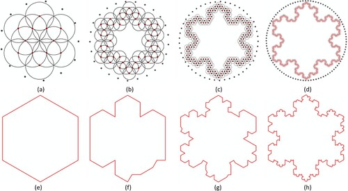
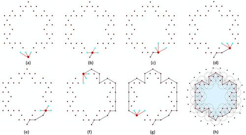
The next step is to delimit the boundary of each derived cluster. As each detected cluster can be in any arbitrary shape, we tend to find a relatively accurate approach to derive polygons from its contained points. The simplest way to solve this problem is convex hull (Jarvis 1973), although this will usually generate quite a lot of lacunas, leading to inaccurate delimitation, and even worse, potential overlaps with nearby clusters. The concave hull was invented to overcome such a problem, but it sometimes suffers from multiple resulting boundaries that are dependent on the number of points used. The study makes use of the k-nearest neighbor approach by Moreira and Santos (2007). Figure 3 demonstrate the outlining process of the points of Koch snowflake at the second level in a step-by-step manner. The process begins with lowest point (minimum y) in the cluster and finds its neighbors within a given search radius in the remaining point set as the candidates at the next step. To determine which point to be selected in the candidate set, we adopt the largest anti-clockwise angle from the edge added in the previous step (Figure 3(a–g)). The number of candidates every time is determined by the k value and the given search radius. The process continues iteratively until all points have been traversed. To make sure the boundary shape is as fractal or ‘unsmooth’ as possible, we chose a rigorous setting k = 3 at each iteration unless there was no eligible point within the temporary computed hull (k value is increased in such cases). By doing so, the shape of derived concave hull can gradually approximate a fractal-like shape (such as a Koch snowflake), given the increasing number of points with a convoluted spatial distribution (Figure 2(e–h)). Note that the smaller the k parameter is, the concave shape becomes increasingly convoluted. However, a small value of k could result in an asymmetrical shape, even when the point set is symmetric (as illustrated in Figure 3). This occurs because next selected point is determined by a local ‘largest-angle’ decision rather than a global one.

Figure 3. (Color online) The demonstration of concave hull delimitation process for vertices of Koch snowflake of level 2.

2.3. Intra-urban scaling analytics for the detected clusters

2.3.1 Power law distribution for single within-cluster attributes

A power law model can be expressed by a probability distribution, as in Equation (1): (1) $\mathrm{p}(\mathrm{x})\propto {\mathrm{x}}^{-\alpha }$(1) Equation (1) denotes the probabilities of a value being proportional to some power of a quantity (x). The easiest way to identify whether a data follows a power law distribution is to rank the data elements in descending order and plot the sorted sequence with double logarithms. If the plot appears a straight line, the distribution is probably a power law. However, this line often fails to be straight because most datasets plotted in such a manner have fluctuated tails (Newman 2005). To overcome such an issue, several algorithms can be employed to estimate the power exponent values, such as the least squares method (LSM) and maximum likelihood method (MLE, Newman 2005; Clauset, Shalizi, and Newman 2009). If the residuals of the observational data are normally distributed, MLE proves to be equivalent to LSM (Charnes, Frome, and Yu 1976). This study adopts MLE to examine power law of a single observational variable by assuming its normality is not met.

MLE estimates the power law exponent, $\alpha$, using smallest data value ${\mathrm{x}}_{\min }$ from where the data is power-law distributed. The exponent $\alpha$ is described as in Equation (2): (2) $\alpha =1+\mathrm{n}{\left[\sum _{\mathrm{i}=1}^{\mathrm{n}}\ln {\displaystyle \frac{{\mathrm{x}}_{\mathrm{i}}}{{\mathrm{x}}_{\min }}}\right]}^{-1}$(2)

The common range of exponent value is between 1 and 3. As a power law distribution demonstrates a substantial imbalance or heterogeneity, we can say that the more heterogenous the data, the larger the exponent will be. Furthermore, to evaluate the adherence of empirical data to an ideal power-law model fitted with ${\mathrm{x}}_{\min }$ and $\alpha$ values, a modified Kolmogorov–Smirnov test suggested by Clauset, Shalizi, and Newman (2009) can be utilized. Simply put, this test involves generating numerous synthetic datasets that conform to a perfect power-law above ${\mathrm{x}}_{\min }$, while retaining the same non-power-law distribution as the original dataset below ${\mathrm{x}}_{\min }$. By comparing the synthetic datasets to the fitted model and calculating the maximum difference between them, the goodness-of-fit index p-value can be obtained. The p-value ranges from 0 to 1 and is determined by calculating the ratio of the number of synthetic datasets that display a greater maximum difference than the original dataset to the total number of synthetic datasets. A p-value of 0 signifies the rejection of the hypothesis that the dataset follows a power-law distribution. This procedure is repeated 1000 times to ensure accuracy. In this study, the baseline of p-value is set as no smaller than 0.05. This means that among 1000 synthetic datasets, at least 50 should have a weaker power-law distribution than the original dataset, thereby suggesting the original data obeys a power law distribution.

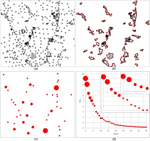
In recent years, the invention of the ht-index (Jiang and Yin 2014) has greatly helped to characterize the extent to which data being power-law-distributed. To calculate the ht-index, it is necessary to apply the head/tail breaks method (Jiang 2013) on the data with a heavy-tailed distribution. In short, the data can first be bisected into a few large values (head) and a great many small values (tail) at the arithmetic mean. The dividing process continues to head recursively until the head is no longer the minority. When the process finishes, the ht-index value is equal to the number of times data can be partitioned plus one. In other words, the ht-index can measure the fractality of a one-dimensional numerical value array sorted in descending order by counting the recurrence of disproportional large-to-small ratios within the data – statistical self-similarity. The larger the ht-index, the greater the chance that data will be more heterogenous or power-law-like. Note that the value range of ht-index is from 1 to $+\mathrm{\infty }$, so the ht-index is more capable of differentiating two power-laws with relatively closer exponents. The traditional threshold for determining a group of values being a head is less than 40 percent. Figure 4 demonstrates how the scaling analysis applies to detected urban clusters. For each cluster, we computed the number of street junctions and population it contains, as well as its area. Then we rank the clusters regarding each of these attributes from largest to smallest and conduct power law detection and head/tail breaks to compute three parameters: the power law exponent $\alpha$, the goodness-of-fit index p-value, and the ht-index value ht. As it is well-known that the power law also refers to the Pareto distribution (Dunford, Su, and Tamang 2014), we apply a strict percentage setting of 20 percent for head/tail partition according to the 20/80 rule or Pareto Principle. This way the derived ht value can reflect the inherent hierarchy of intra-urban clusters.

Figure 4. (Color online) Illustration of scaling analysis on detected urban clusters (Note: Given a set of street junctions (Panel a), we first conduct the clustering and compute the boundary for each cluster (Panel b), and then assign the attributes on those clusters, represented by dot sizes (Panel c). Finally, we compute long-tailed statistics using head/tail divisions applying on the rank-size plot of cluster attributes, from which the two heads are recursively derived, resulting in a ht-index value of 3 (Panel d)).

2.3.2 Intra-urban scaling law examined using within-cluster attributes

With the progressively increasing distance threshold, it becomes possible to describe more precisely the allometric growth between urban functions and city size over ‘space’. The urban allometric scaling relationship can be modeled using power function fitting between two types of urban quantities across derived intra-urban clusters, denoted as Equation (3): (3) $\mathrm{Y}(\mathrm{d})=\mathrm{kN}(\mathrm{d}{)}^{\beta }$(3) where $\mathrm{Y}(\mathrm{d})$ and $\mathrm{N}(\mathrm{d})$ are the computed value of the urban within-cluster attribute and the population at clustering cutoff distance $\mathrm{d}$, respectively, and $\beta$ is the scaling exponent and $k$ is the constant.

The scaling exponent $\beta$ can be categorized into three schemes: the sub-linear ($\beta <1$), linear ($\beta \approx 1$), and super-linear ($\beta >1$) scaling relationships between urban measures (Bettencourt et al. 2007). Each scheme relates to urban functions or performances of different kinds. Along with population growth, the sub-linear relationship is often used to refer to the lower demand for infrastructure and built-up area because of economies of scale and spatial agglomerations, while the super-linear relationship indicates the increasing returns to scale and the internal interactions (Bettencourt 2013; Batty 2013). In theory, the ideal sublinear scaling exponent values for matured urban system are around 5/6 (0.83) for infrastructure and 2/3 (0.67) for urban area, while the super-linear one is about 7/6 (1.17) for GDP (Zünd and Bettencourt 2019; Liu et al. 2022). In this study, we use the clusters derived at each distance cutoff as alternative spatial units to examine the allometric scaling relationship at the intra-urban level. To do this, we conduct the power function fitting between population and three urban metrics (such as number of street junctions, GDP, and area) that are within each intra-urban cluster. The scaling exponent $\beta$ is the slope of the straight line in the log–log graph according to Equation 3(3) $\mathrm{Y}(\mathrm{d})=\mathrm{kN}(\mathrm{d}{)}^{\beta }$(3) .

3. Experiments and findings

3.1 Overall statistics of derived intra-urban clusters

We started by conducting the clustering using the distance threshold from 100 to 1000 m. Table 1 shows the results in terms of how many clusters were generated from individual road junctions with respect to a series of thresholds at the increment of 100 m. The number of clusters drops dramatically from 100 m to 300 m, and continuously but slowly till 400 m. We also checked the maximum number of points in each cluster set. Both the number of clusters and the maximum number of points decreased flatly after 400 m. This observation is valid for both cities. We also checked how much area the cluster set occupied over the entire city. Interestingly, when reaching 400 m, the occupied ratio for Shenzhen is about 80 percent, whereas the equivalent figure for Beijing is only around 30 percent (Figure 5(a)). However, the number of road junctions within the largest cluster for each city already accounted for a considerable part of all junctions. In this respect, the forms between two cities show a significant difference.

Figure 5. (Color online) Progressively generated intra-urban clusters derived using the clustering distance threshold from 100 m to 400 m (a) and largest clusters using 200 m threshold and their contained streets and junctions in Shenzhen (b) and Beijing (c), respectively.

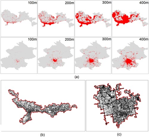
Table 1. Overall statistics of derived urban clusters at different thresholds.

Distance	#Clusters (Beijing)	Max #Points (Beijing)	#Clusters (Shenzhen)	Max #Points (Shenzhen)
100	27,754	1170	10,873	1602
200	14,208	40,659	3503	19,443
300	8057	63,894	1373	23,385
400	4799	82,358	632	39,768
500	3161	93,594	340	44,985
600	2288	105,920	210	45,612
700	1712	113,718	145	45,933
800	1368	117,676	110	46,077
900	1116	119,626	87	46,225
1000	918	125,241	69	46,835

(Note: # = number, Max #Points = Number of points in the largest cluster).

3.2 Findings based on the scaling distribution of within-cluster attributes

In what follows, we demonstrate how power-law-related metrics on four attributes alters with respect to the threshold distance. Before that, we applied the robust power law detection based on the MLE method and head/tail breaks based on the 80/20 principle to examine whether the distribution of the metrics shows a universal regularity of power law regarding each cluster set derived at 100, 200, 300, and 400 m, respectively (Figure 6). Table 2 shows the scaling metrics for each of four attributes of urban clusters. Most of the cluster sets were power-law-distributed for both cities. The exponent values ($\alpha$) were largely around 2, and the p-values mostly were above 0.05. Despite being calculated using a very strict ratio (20 percent), the ht-index was larger than or equal to 3 in most cases. For a cluster set whose attributes did not pass the power law test, the ht-index was most likely below 3 (for example, population for clusters at 100 m distance threshold in Beijing; Table 2(a)). It is also interesting to note that both power law exponents and the ht-index values of population showed less heterogeneity than those of GDP, number of street nodes, and area, respectively.

Figure 6. (Color online) Power law distribution of cluster size (area) with respect to different clustering resolutions from 100 m to 400 m for Beijing (a) and Shenzhen (b).

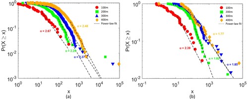
Table 2. Scaling statistics of four attributes within the intra-urban clusters generated at different distance cutoffs from 100 m to 400 m for Beijing (a) and Shenzhen (b)

(a)
	#Junctions			Area			Population			GDP
	$\alpha$	p	ht	$\alpha$	p	ht	$\alpha$	p	Ht	$\alpha$	p	ht
100m	2.49	0.30	2	2.67	0.22	2	1.42	0.01	1	2.39	0.14	5
200m	2.29	0.11	5	2.29	0.20	4	1.69	0.12	2	2.21	0	4
300m	2.30	0.82	4	2.37	0.91	4	2.08	0.80	3	2.22	0.02	3
400m	2.29	0.72	4	2.48	0.76	4	1.68	0	3	2.52	1	3
(b)
	#Junctions			Area			Population			GDP
	$\alpha$	p	ht	$\alpha$	p	ht	$\alpha$	p	Ht	$\alpha$	p	ht
100m	2.56	0.96	2	2.39	0.70	3	1.94	0.62	2	3.39	0.47	3
200m	2.11	0.80	4	1.82	0	4	2.04	0.49	3	2.22	0.83	3
300m	1.86	0.82	4	1.85	0.93	4	1.65	0.84	3	2.01	0.3	4
400m	1.94	0.12	3	1.77	0.80	3	1.51	0.44	2	1.83	0.66	3

To obtain a more nuanced understanding of how scaling patterns relate to clustering distances, we derived clusters by increasing the threshold, one at a time, between 100 and 400, and conducted scaling analysis for each of the four attributes for each cluster set accordingly. Figure 6 shows a detailed view on the change of scaling metrics of three attributes (street nodes in blue, area in gray, population in orange, GDP in green) of derived urban clusters along with the increase of clustering distance in Beijing and Shenzhen. Overall, although the curves by $\alpha$ and ht of GDP went beyond 3 at the very beginning, the curves between the number of street nodes and cluster areas show good consistency. In Beijing, exponents for each of two attributes peaked at 2.6 between 150 and 200 m, stabilized around 2.3 between 200 and 300 m, then decreased but fluctuated between [2, 2.4] afterwards (Figure 7(a)); In Shenzhen, those two curves largely showed a decreasing trend from 2.6 to 1.8 (Figure 7(c)). Correspondingly, ht of two attributes in both cities were very low (1) at the beginning and increased rapidly towards values of 3 or 4 from 100 to 150 m, and then became stable at values of 4 and 5 after 200 m, respectively (Figure 7(b and d)).

Figure 7. (Color online) A detailed view of the change of power law metrics of four attributes (#street nodes, area, population, and GDP) within derived urban clusters, along with the increase of clustering distance in Beijing (Panels a and b) and Shenzhen (Panels c and d). (Note: The x-axes all represent the clustering distance from 100 to 400 meters and the y-axes are power law exponent (Panels a and c) and ht-index (Panels b and d), respectively).

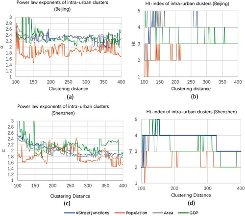
However, there is a significant difference when comparing the scaling metrics of population with those of other three attributes in the course of the progressive clustering. For $\alpha$, in both cities, despite more ups and downs, the exponent values of population were generally less than another three attributes; For ht, the maximum values in both cities were only 3, whereas for other three attributes were peaked at 5.

3.3 Findings based on the scaling relations between intra-urban quantities

Having examined the scaling distribution of cluster-related attributes, we investigated how the process of these metrics becoming gradually ‘saturated’. Figure 8 showed that the growth of cluster size paced differently with other three measures. In Beijing, for instance, an average of approximately 15 percent of urban land was responsible for more than 50 percent of urban functions (Table 3), which significantly demonstrated the spatial agglomeration effect. In Shenzhen, the slopes of increase between urban area and functions were much more coordinated. We further computed $\beta$ regarding three metrics against population at the cluster level to examine intra-urban scaling law. Among three urban metrics, we assumed that GDP, number of street junctions, and the size of derived cluster are respective proxies of socio-economic status, infrastructure, and the urban built-up area. In sum, the goodness of the power function fitting (R²) in Shenzhen was always higher than that in Beijing. In addition, for both cities, the variables related to socio-economy were with lower R² value than variables of infrastructure and built-up area. For example, in Shenzhen, of all the urban functions delimited by different clustering distances ranging from 100 to 1000, the scaling relationship between the number of junctions and population was largest (R² = 0.79 ± 0.12), while that between GDP and population was the smallest (R² = 0.51 ± 0.18).

Figure 8. (Color online) The plot for the proportions regarding four attributes with the increasing clustering distance in Beijing (a) and Shenzhen (b).

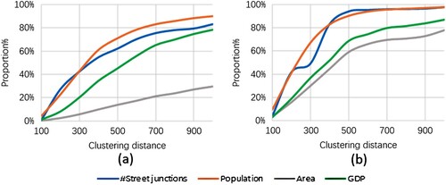
Table 3. The proportion of metrics within clusters at different distance thresholds to that of the entire city (Note: Pop = Population; # = number).

Beijing					Shenzhen
Distance	Area%	#Junction%	GDP%	Pop%	Area%	#Junction%	GDP%	Pop%
100	0.49%	0.82%	1.37%	4.27%	3.24%	3.89%	3.07%	9.65%
300	5.86%	42.42%	20.38%	42.98%	29.91%	49.24%	36.92%	67.41%
500	13.87%	61.98%	45.13%	71.18%	59.06%	94.06%	68.66%	90.47%
700	21.16%	75.25%	65.01%	83.24%	69.55%	95.88%	79.69%	95.91%
900	26.96%	79.17%	74.54%	88.49%	72.80%	96.43%	83.71%	97.26%

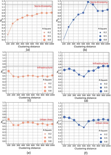
As shown in Figure 9, $\beta$ changed across three urban attributes against population with varied clustering distances. The trajectories of $\beta$ changes between two cities were strikingly different, where we can see that the curve for Beijing was nearly flat and almost always under the theoretical value of either super-linear or sub-linear scheme, whereas the curve of $\beta$ for Shenzhen went above and beneath the theoretical reference line from distance to distance. Moreover, it is striking to observe that a tipping point of clustering distance in Shenzhen was found around 500 or 600 m for all three types of urban functions. As the distance increased, either the socioeconomic or the infrastructure attributes got closer to the theoretical super-linear or sub-linear line.

Figure 9. (Color online) The change of allometric scaling relationships for within-cluster GDP, street junction, and area versus within-cluster population at different distance thresholds (Note: the theoretical relationship for each urban function type was drawn as a reference line (7/6 for socio-economy; 5/6 for infrastructure; 2/3 for area) in each plot).

4. Discussion of this study

Urban phenomena are categorized into two branches: with and without a characteristic scale (Chen 2021). The characteristic scale refers to the well-defined average that can be conveniently identified in a normal distribution and its variants. However, city, as a complex spatial system manifested by its fractal shapes and heavy-tailed distribution statistics (either power laws or being akin to the power law), often bears no characteristic scale, or its measurement depends sensitively on the measuring scale. In this connection, we can view these two branches as simple and complex aspects of a city: Two aspects co-exist and are not contradictory, just as a fractal shape is made of simple geometric primitives. However, conventional mathematical and quantitative methods are capable of handling the simple aspect rather than the complex one. To address the issue, recent literature managed to decompose a power law into a pair of exponential distributions in which a characteristic scale can be identified (Chen 2015) and later found it effective for urban boundary delineation (Chen et al. 2022). With the focus mainly being on the city’s complex sides, we adopt progressive spatial clustering approach that treats all scales as a whole for urban characterization and, thus, the identification of the characteristic scale fell outside the scope of this work.

The fractal-geometric thinking underlies the progressively generated intra-urban clusters. Most conventional geospatial models are based on Euclidean geometries – being simple, regular, or smooth, such as equally partitioned cells or top-down imposed administrative boundaries. Although remarkable outputs were achieved, these units still have certain inadequacies. As Alexander (2005) stated, ‘these things of this world, do not have the idealized shapes, and Euclid’s geometry comes nowhere near being able to describe them’. The clusters as the modeling units in this study were determined in a totally bottom-up manner – that is, by straight-line distance between every pair of street junctions – shaped by the concave hull approach. Geometrically, the computed concave boundaries of each cluster accurately reflect the picture of the fractal intra-urban forms that are irregular, rough, and convoluted, conforming to previous NC and hotspot detection approaches (e.g. Jiang and Jia 2011; Ma et al. 2021) but at a more detailed level. Mathematically, the fractal-geometric perspective of cluster patches can be thoroughly understood from two statistical angles: the power law of patch sizes and the allometric relationship between patch sizes and scales at which each size is measured (such as fractal dimension). The former angle enables us to characterize urban form based on the cluster size or other associated attribute alone and the latter one allows us to examine systematically the intra-urban scaling law using within-cluster attributes against population. It should be noted that the application of Euclidean distance is to identify clusters as urban populous areas in a broader context, encompassing various urban features and their interactions. On the other hand, clusters identified using other distance types, such as network steps and temporal distances, tend to focus more on travel-related activity and may be less effective in characterizing urban form.

The progressive clustering process of street junctions resembles the sandpile experiment in which sand is persistently accumulated into differently sized avalanches that exhibit power law behavior (Bak 1996). Figure 6(a and c) show that mostly $\alpha$ did not deviate much from 2 across different attributes upon the growth of clusters, which is akin to the best-known inter-urban scaling property – Zipf’s law for city size distribution – where $\alpha$ is around 2 in a probability distribution (Zipf 1949; Newman 2005). Zipf’s law has been validated for cities at regions, countries, continents, and even at the global level. This study exemplifies such a statistical regularity within a city that further strengthens the self-similar hierarchy of geographic space. Differently sized concentrations of high/low densities of street intersections behind Zipf’s law can help us adapt the 20/80 principle to characterize the urban form. As is the case with ht, which is calculated using a 20 percent threshold for determining the head (places with high concentrations), the value of 4 or 5 indicates a striking power law distribution or a tightly resembling one with a great heterogeneity and a steep hierarchy of intra-urban cluster sizes. Thus, we can identify that the spatial distribution of detected clusters in Beijing and Shenzhen has a giant concentration in the city center and many small ones scattered around (Figure 5). What is interesting is that larger $\alpha$ and ht are along with a longer series of distance thresholds in Beijing than those in Shenzhen (Figure 7(b and d)). This means that Shenzhen has a more even or dispersed distribution of concentrations and further implies a more polycentric urban structure than Beijing. Furthermore, it is worth noting that the ht-index outperforms $\alpha$ when making comparisons. Figure 7 clearly demonstrates that while α appears to be seldom exceeds 3, the ht-index exhibits a greater value range. This suggests that ht has the potential to differentiate between two power-laws that have a similar $\alpha$ value, and in the meantime better reflects the underlying data hierarchy.

Throughout the clustering process, ht for population is always lower than other three attributes, clearly showing the allometric growth of different types of urban quantities accompanying the increasing cluster sizes. Comparing the ratio of each within-cluster attribute to the entire city, we can notice an imbalanced urban development in two metropolises, that is, a relatively small part of urban area accounted for a significant part of the urban population and wealth, especially at the distance from 100 to 400 m. This reconfirms that each part of a city is not with a ‘synchronized’ development (Alvioli 2020). As the clustering distance grows, such an imbalance for ratios of area and other measures remained steady in Beijing but gradually alleviated in Shenzhen. This again suggests the difference between monocentric and polycentric development patterns. Further, the progressively generated clusters allow us to observe the spectrum of $\beta$ in both cities. Referenced by the theoretical value for developed cities (Zünd and Bettencourt 2019; Liu et al. 2022), despite being greatly concentrated, the smaller $\beta$ of socio-economy and infrastructure in Beijing (Figure 9(a and c)) suggest an immature urban system, because less per-capita GDP and utility can be provided. In Shenzhen, the scaling exponents for GDP dramatically increased at the beginning from a sub-linear behavior, to a super-linear one that peaked at 600 m, and then decreased to sub-linear after 700 m (Figure 9(b)). 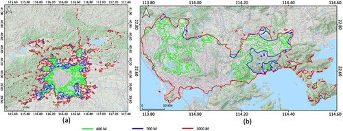The sharply increased $\beta$ in the threshold range of 100–600 m showcase the per-capita urban economic efficiency. One reason could be the decentralized urban form in Shenzhen offers greater accessibility for people to move within and across different parts of the city, thus facilitating easier connections between people and businesses and resulting in more productive economic activity. As half of the administrative area in Shenzhen is covered by ecological regions (Shi and Yu 2014), the weakened scaling relationships (not only GDP but also other two metrics) were probably due to the topographical constraints. Namely, clusters derived after 600 m included considerably ‘ineffective’ areas that affect the theoretical super-linear scaling relationship for GDP, while it was not the case in Beijing (Figure 10). With the above observed insights, echoed with the prior study by Molinero and Thurner (2021), the presence of scaling law determined by each intra-urban cluster set makes it possible to explore the system of any individual city from such a fractal-geometric perspective.

Figure 10. (Color online) The growth of concave cluster boundaries after 400 m overlapped with the topographic map in Beijing (a) and Shenzhen (b).

5. Conclusion and future work

Urban space is filled with great heterogeneity or complexity in geometry or in statistics (Wen and Li 2021), and is therefore essentially fractal or scaling in nature. To effectively investigate the fractal urban form and power law statistics therein, we adopted novel spatial modeling units by clustering street junctions that are consistent with varying densities at the intra-city scale. By exploring these patterns of intra-urban clustering, it is possible to gain insights into the fundamental mechanisms that underlie the evolution of urban spatial structure. We observed the emergence of the ‘power law regularity’ from simple clustering operations; that is, the probable universal existence of power law distribution regarding four attributes – number of street junctions, cluster size, population, and GDP – over the urban space.

As noted, power law distribution of urban facts showcases a tendency towards structural optimization, implying a sustainable configuration behind a long run of self-organized and the adaptive processes (Batty, Longly, and Fotheringham 1989). It was also intriguing to find that those power laws differ from attribute to attribute or city to city with fluctuated exponents and ht-index values under every clustering distance threshold setting. The comparison among profiles of power-law-related metrics can be further used to characterize the mono or polycentric urban structure. Cities that adopt a polycentric form tend to be more efficient and sustainable and to have better urban performance (Burger and Meijers 2012; Yue et al. 2023) because of greater accessibility between people and places. This can be further confirmed by the examination of intra-urban scaling laws given the allometric growth among different urban measures within progressively generated clusters. As the case with GDP, by comparing the spectrums of scaling exponents upon the cluster growth in both cities, we found that Shenzhen exhibits a higher urban economic efficiency by surpassing the well-defined super-linear scheme. After understanding how the city’s structure relates to its functions from such a fractal or scaling perspective, policymakers can make informed decisions about urban planning and development to ensure if the city meets the needs of its residents.

Future work will involve more sophisticated clustering criteria, such as considering network or temporal distance types (Black and Wachowicz 2021) for some specific urban scenarios (such as human mobility analysis). In addition, further exploration of the mechanisms of how different power law exponents among the four types functional attributes associate with their scaling relations in the intra-urban system is required. The study will also be extended to involve more domestic and overseas cities with different levels of development status quo and to formulate an international outlook of the intra-urban fractal or scaling structures.

Acknowledgements

The authors would like to thank the editor and all reviewers for their constructive and insightful comments that significantly improve this study.

Disclosure statement

No potential conflict of interest was reported by the author(s).

Data availability statement

The data and cluster results that support the findings in this study are available on figshare. The link to data and cluster results: https://doi.org/10.6084/m9.figshare.19153886.v1.

Additional information

Funding

This study is supported and funded by the National Natural Science Foundation of China (No.42001180); Shenzhen Science and Technology Program (No. 20220809120650001); Guangdong Science and Technology Strategic Innovation Fund (the Guangdong-Hong Kong-Macau Joint Laboratory Program, No. 2020B1212030009).

References

- Alexander, C. 2005. The Nature of Order: An Essay on the Art of Building and the Nature of the Universe. Berkeley, CA: Center for Environmental Structure.
- Alvioli, M. 2020. “Administrative Boundaries and Urban Areas in Italy: A Perspective from Scaling Laws.” Landscape and Urban Planning 204: 103906. doi:10.1016/j.landurbplan.2020.103906.
- Arcaute, E., E. Hatna, P. Ferguson, H. Youn, A. Johansson, and M. Batty. 2015. “Constructing Cities, Deconstructing Scaling Laws.” Journal of The Royal Society Interface 12: 20140745. doi:10.1098/rsif.2014.0745.
- Bak, P. 1996. How Nature Works: The Science of Self-Organized Criticality. New York: Springer-Verlag.
- Batty, M. 2013. “A Theory of City Size.” Science 340 (6139): 1418–1419. doi:10.1126/science.1239870.
- Batty, M., R. Carvalho, A. Hudson-Smith, R. Milton, D. Smith, and P. Steadman. 2008. “Scaling and Allometry in the Building Geometries of Greater London.” The European Physical Journal B 63: 303–314. doi:10.1140/epjb/e2008-00251-5.
- Batty, M., and P. Longley. 1997. Fractal Cities: A Geometry of Form and Function. London: Academic Press. doi:10.1016/S0264-2751(97)89331-6
- Batty, M., P. Longly, and S. Fotheringham. 1989. “Urban Growth and Form: Scaling, Fractal Geometry, and Diffusion-Limited Aggregation.” Environment and Planning A: Economy and Space 21 (11): 1447–1472. doi:10.1068/a211447.
- Bennett, J. 2010. OpenStreetMap: Be Your own Cartographer. Birmingham: PCKT Publishing.
- Bettencourt, L. M. 2013. “The Origins of Scaling in Cities.” Science 340 (6139): 1438–1441. doi:10.1126/science.1235823.
- Bettencourt, L. M. A., J. Lobo, D. Helbing, C. Kühnert, and G. B. West. 2007. “Growth, Innovation, Scaling, and the Pace of Life in Cities.” Proceedings of the National Academy of Sciences 104 (17): 7301–7306. doi:10.1073/pnas.0610172104.
- Bettencourt, L. M., J. Lobo, D. Strumsky, and G. B. West. 2010. “Urban Scaling and its Deviations: Revealing the Structure of Wealth, Innovation and Crime Across Cities.” PloS one 5 (11): e13541. doi:10.1371/journal.pone.0013541.
- Black, K., and M. Wachowicz. 2021. “Clustering Spatio-Temporal bi-Partite Graphs for Finding Crowdsourcing Communities in IoMT Networks.” Big Earth Data 5 (1): 24–48. doi:10.1080/20964471.2021.1899578.
- Burger, M., and E. Meijers. 2012. “Form Follows Function? Linking Morphological and Functional Polycentricity.” Urban Studies 49 (5): 1127–1149. doi:10.1177/0042098011407095.
- Charnes, A., E. L. Frome, and P. L. Yu. 1976. “The Equivalence of Generalized Least Squares and Maximum Likelihood Estimates in the Exponential Family.” Journal of the American Statistical Association 71: 169–171. doi:10.1080/01621459.1976.10481508.
- Chen, Y. 2011. “Fractal Systems of Central Places Based on Intermittency of Space-Filling.” Chaos, Solitons & Fractals 44 (8): 619–632. doi:10.1016/j.chaos.2011.05.016.
- Chen, Y. 2015. “Power-law Distributions Based on Exponential Distributions: Latent Scaling, Spurious Zipf’s law, and Fractal Rabbits.” Fractals 23 (2): 1550009. doi:10.1142/S0218348X15500097.
- Chen, Y. 2021. “Characteristic Scales, Scaling, and Geospatial Analysis.” Cartographica: The International Journal for Geographic Information and Geovisualization 56 (2): 91–105. doi:10.3138/cart-2020-0001.
- Chen, Y., Y. Wang, and X. Li. 2019. “Fractal Dimensions Derived from Spatial Allometric Scaling of Urban Form.” Chaos, Solitons & Fractals 126: 122–134. doi:10.1016/j.chaos.2019.05.029.
- Chen, Y., J. Wang, Y. Long, X. Zhang, and X. Li. 2022. “Defining Urban Boundaries by Characteristic Scales.” Computers, Environment and Urban Systems 94: 101799. doi:10.1016/j.compenvurbsys.2022.101799.
- Christaller, W. 1933. Central Places in Southern Germany. Prentice Hall: Englewood Cliffs, N. J.
- Clauset, A., C. Shalizi, and M. Newman. 2009. “Power-law Distributions in Empirical Data.” Society for Industrial and Applied Mathematics 51 (4): 661–703. doi:10.48550/arXiv.0706.1062.
- Dunford, R., Q. Su, and E. Tamang. 2014. The Pareto Principle. Plymouth: University of Plymouth.
- Goodchild, M. F. 2004. “The Validity and Usefulness of Laws in Geographic Information Science and Geography.” Annals of the Association of American Geographers 94 (2): 300–303. doi:10.1111/j.1467-8306.2004.09402008.x.
- Jacobs, J. 1961. The Death and Life of Great American Cities. New York: Random House.
- Jarvis, R. A. 1973. “On the Identification of the Convex Hull of a Finite set of Points in the Plane.” Information Processing Letters 2 (1): 18–21. doi:10.1016/0020-0190(73)90020-3.
- Jiang, B. 2013. “Head/Tail Breaks: A new Classification Scheme for Data with a Heavy–Tailed Distribution.” The Professional Geographer 65 (3): 482–494. doi:10.1080/00330124.2012.700499.
- Jiang, B., and T. Jia. 2011. “Zipf's law for all the Natural Cities in the United States: A Geospatial Perspective.” International Journal of Geographical Information Science 25 (8): 1269–1281. doi:10.1080/13658816.2010.510801.
- Jiang, B., and Y. Miao. 2015. “The Evolution of Natural Cities from the Perspective of Location-Based Social Media.” The Professional Geographer 67 (2): 295–306. doi:10.1080/00330124.2014.968886.
- Jiang, B., and J. Yin. 2014. “Ht–Index for Quantifying the Fractal or Scaling Structure of Geographic Features.” Annals of the Association of American Geographers 104 (3): 530–540. doi:10.1080/00045608.2013.834239.
- Krugman, P. 1996. “Confronting the Mystery of Urban Hierarchy.” Journal of the Japanese and International Economies 10: 399–418. doi:10.1006/jjie.1996.0023.
- Lan, T., Z. Li, and H. Zhang. 2019. “Urban Allometric Scaling Beneath Structural Fractality of Road Networks.” Annals of the American Association of Geographers 109 (3): 943–957. doi:10.1080/24694452.2018.1492898.
- Liu, Z., H. Liu, W. Lang, S. Fang, C. Chu, and F. He. 2022. “Scaling law Reveals Unbalanced Urban Development in China.” Sustainable Cities and Society 87: 104157. doi:10.1016/j.scs.2022.104157.
- Long, Y., W. Zhai, Y. Shen, and X. Ye. 2018. “Understanding Uneven Urban Expansion with Natural Cities Using Open Data.” Landscape and Urban Planning 177: 281–293. doi:10.1016/j.landurbplan.2017.05.008.
- Ma, D., R. Guo, Y. Jing, Y. Zheng, Z. Zhao, and J. Yang. 2021. “Intra-Urban Scaling Properties Examined by Automatically Extracted City Hotspots from Street Data and Nighttime Light Imagery.” Remote Sensing 13 (7): 1322. doi:10.3390/rs13071322.
- Ma, D., M. Sandberg, and B. Jiang. 2017. “A Socio-Geographic Perspective on Human Activities in Social Media.” Geographical Analysis 49 (3): 328–342. doi:10.1111/gean.12122.
- Ma, D., O. Toshihiro, T. Oki, and B. Jiang. 2020. “Exploring the Heterogeneity of Human Urban Movements Using geo-Tagged Tweets.” International Journal of Geographical Information Science 34 (12): 2475–2496. doi:10.1080/13658816.2020.1718153.
- Makse, H. A., J. S. Andrade, M. Batty, S. Havlin, and H. E. Stanley. 1998. “Modeling Urban Growth Patterns with Correlated Percolation.” Physical Review E 58 (6): 7054. doi:10.1103/PhysRevE.58.7054.
- Mandelbrot, B. 1967. “How Long is the Coast of Britain? Statistical Self-Similarity and Fractional Dimension.” Science 156: 636–638. doi:10.1126/science.156.3775.636.
- Masucci, A. P., E. Arcaute, E. Hatna, K. Stanilov, and M. Batty. 2015. “On the Problem of Boundaries and Scaling for Urban Street Networks.” Journal of the Royal Society Interface 12: 20150763. doi:10.1098/rsif.2015.0763.
- Molinero, C., and S. Thurner. 2021. “How the Geometry of Cities Determines Urban Scaling Laws.” Journal of the Royal Society Interface 18 (176): 20200705. doi:10.1098/rsif.2020.0705.
- Montero, G., C. Tannier, and I. Thomas. 2021. “Delineation of Cities Based on Scaling Properties of Urban Patterns: A Comparison of Three Methods.” International Journal of Geographical Information Science 35 (5): 919–947. doi:10.1080/13658816.2020.1817462.
- Moreira, A., and M. Y. Santos. 2007. Concave hull: A k-nearest neighbours approach for the computation of the region occupied by a set of points.
- Naroll, R. S., and B. L. Von. 1973. “The Principle of Allometry in Biology and the Social Sciences.” Ekistics; Reviews. on the Problems and Science of Human Settlements, 244–252.
- Newman, M. 2005. “Power Laws, Pareto Distributions and Zipf’s law.” Contemporary Physics 46: 323–351. doi:10.1080/00107510500052444.
- Ren, Z. 2018. Toolbox for Extracting Street Nodes from OSM Data and Creating Natural Cities from Street Nodes Using ArcGIS Model. https://www.arcgis.com/home/item.html?id = 47b1d6fdd1984a6fae916af389cdc57d.
- Rozenfeld, H. D., D. Rybski, J. S. Andrade, M. Batty, H. E. Stanley, and H. A. Makse. 2008. “Laws of Population Growth.” Proceedings of the National Academy of Sciences 105 (48): 18702–18707. doi:10.1073/pnas.0807435105.
- Shi, P., and D. Yu. 2014. “Assessing Urban Environmental Resources and Services of Shenzhen, China: A Landscape-Based Approach for Urban Planning and Sustainability.” Landscape and Urban Planning 125: 290–297. doi:10.1016/j.landurbplan.2014.01.025.
- Shreevastava, A., P. S. C. Rao, and G. S. McGrath. 2019. “Emergent Self-Similarity and Scaling Properties of Fractal Intra-Urban Heat Islets for Diverse Global Cities.” Physical Review E 100: 032142. doi:10.1103/PhysRevE.100.032142.
- Stevens, F. R., A. E. Gaughan, C. Linard, and A. J. Tatem. 2015. “Disaggregating Census Data for Population Mapping Using Random Forests with Remotely-Sensed and Ancillary Data.” Plos one 10 (2): e0107042. doi:10.1371/journal.pone.0107042.
- Tannier, C., and I. Thomas. 2013. “Defining and Characterizing Urban Boundaries: A Fractal Analysis of Theoretical Cities and Belgian Cities.” Computers, Environment and Urban Systems 41: 234–248. doi:10.1016/j.compenvurbsys.2013.07.003.
- Tannier, C., I. Thomas, G. Vuidel, and P. Frankhauser. 2011. “A Fractal Approach to Identifying Urban Boundaries. 城市边界识别的分形方法.” Geographical Analysis 43 (2): 211–227. doi:10.1111/j.1538-4632.2011.00814.x.
- Wen, R., and S. Li. 2021. “A Review of the use of Geosocial Media Data in Agent-Based Models for Studying Urban Systems.” Big Earth Data 5 (1): 5–23. doi:10.1080/20964471.2020.1810492.
- West, G. B., J. H. Brown, and B. J. Enquist. 1997. “A General Model for the Origin of Allometric Scaling Laws in Biology.” Science 276 (5309): 122–126. doi:10.1126/science.276.5309.122.
- Yue, W., J. Wei, Y. Liu, T. Wang, and H. Zhang. 2023. “Investigating Intra-Urban Functional Polycentricity from a Linkage Perspective: The Case of Changsha, China.” Journal of Geovisualization and Spatial Analysis 7 (1): 1. doi:10.1007/s41651-023-00132-6.
- Zipf, G. 1949. Human Behavior and the Principle of Least Effort. Cambridge: Addison-Wesley Press.
- Zünd, D., and L. M. A. Bettencourt. 2019. “Growth and Development in Prefecture-Level Cities in China.” PLoS one 14: e0221017. doi:10.1371/journal.pone.0221017.