Generation of global 1-km daily top-of-atmosphere outgoing longwave radiation product from 2000 to 2021 using machine learning

ABSTRACT

Top-of-atmosphere (TOA) outgoing longwave radiation (OLR), a key component of the Earth’s energy budget, serves as a diagnostic of the Earth’s climate system response to incoming solar radiation. However, existing products are typically estimated using broadband sensors with coarse spatial resolutions. This paper presents a machine learning method to estimate TOA OLR by directly linking Moderate Resolution Imaging Spectroradiometer (MODIS) TOA radiances with TOA OLR determined by Clouds and the Earth’s Radiant Energy System (CERES) and other information, such as the viewing geometry, land surface temperature and cloud top temperature determined by Modern-Era Retrospective analysis for Research and Applications, Version 2 (MERRA-2). Models are built separately under clear- and cloudy-sky conditions using a gradient boosting regression tree. Independent test results show that the root mean square errors (RMSEs) of the clear-sky and cloudy-sky models for estimating instantaneous values are 4.1 and 7.8 W/m², respectively. Real-time conversion ratios derived from CERES daily and hourly OLR data are used to convert the instantaneous MODIS OLR to daily results. Inter-comparisons of the daily results show that the RMSE of the estimated MODIS OLR is 8.9 W/m² in East Asia. The developed high resolution dataset will be beneficial in analyzing the regional energy budget.

KEYWORDS:

• TOA outgoing longwave radiation
• MODIS
• CERES
• machine learning
• Earth’s energy budget

1. Introduction

The top-of-atmosphere (TOA) outgoing longwave radiation (OLR), defined as the outgoing radiation flux emitted from the Earth’s surface and atmosphere in the infrared wavelength regime, is an essential component of the Earth’s energy budget (Liang et al. 2019). TOA OLR is widely used in weather and climate research as it is strongly related to atmospheric conditions (e.g. water vapor, cloud cover) (Schmetz and Liu 1988). For instance, OLR has been used as an index of tropical convective activity to investigate decadal variations of atmospheric circulation in the global tropical belt (Nitta and Yamada 1989). Climate changes in the tropical western Pacific and Indian Ocean regions can also be detected by OLR records (Chu and Wang 1997). Therefore, accurate estimation of the global OLR is necessary.

Since the 1980s, many TOA OLR products have been derived from data obtained with broadband sensors, including Earth Radiation Budget Experiment (ERBE) (Barkstrom 1984), Scanner Radiometer for Radiation Budget (ScaRab) (Kandel et al. 1998), Geostationary Earth Radiation Budget (GERB) (Harries et al. 2005), and Clouds and the Earth’s Radiant Energy System (CERES) (Wielicki et al. 1996). Since the 2000s, multispectral narrowband sensors have been incorporated to generate TOA OLR products, including High-Resolution Infrared Radiation Sounder (HIRS) (Lee et al. 2007), Geostationary Operational Environmental Satellite (GOES) Sounder (Ba, Ellingson, and Gruber 2003), GOES-R Advanced Baseline Imager (Lee et al. 2010), Communication Oceanography Meteorological Satellite (COMS) (Park et al. 2015), and Advanced Himawari Imager (AHI) (Kim et al. 2018). These products are generated by the traditional two-step method, which firstly converts radiance into flux and then obtains the TOA OLR using the derived flux. Since these two independent procedures could bring extra errors separately, accumulation of errors would occur in the final estimated TOA OLR values. Moreover, existing retrieval algorithms are usually based on regression analyses of radiative transfer simulations, and numerous products with coarse spatial resolutions are derived from observed broadband fluxes from sensors specifically designed to measure the entire infrared spectrum. CERES OLR datasets have been recognized as the most accurate products, but the spatial resolution of CERES products is rather coarse (at least 20-km), and the time span is quite short (starting from 2000) (Wang et al. 2021; Zhan et al. 2019). Thus, to better analyze the Earth’s energy budget at regional scales, high spatial resolution (1-km) TOA OLR dataset with high accuracy is needed.

A novel algorithm for TOA albedo retrieval, which directly links Advanced Very High Resolution Radiometer (AVHRR) narrowband reflectances with CERES TOA broadband albedos, was proposed in our previous study (Zhan and Liang 2022). This study presents a companion work in terms of TOA OLR. Herein, Moderate Resolution Imaging Spectroradiometer (MODIS) data are used instead of AVHRR data because MODIS has 16 thermal infrared (TIR) channels, which are necessary for TOA OLR retrieval. Additionally, despite its unique long time span, the quality of AVHRR data is worse than MODIS data, and satellite orbital drift is also a notable problem (Liu et al. 2019). In our previous study (Zhan and Liang 2022), AVHRR–CERES data pairs could only be collected in certain years, i.e. only when the orbital planes of the Terra/Aqua and NOAA satellites coincided. For MODIS–CERES data pairs, however, collecting collocated pairs is much easier as MODIS and CERES are located on the same satellite.

Machine learning methods can learn the relationship between inputs and outputs by fitting flexible models to data. This study presents a refinement of machine learning practices of our previous study, in which collocated AVHRR-CERES data pairs were collected to build machine learning models (Zhan and Liang 2022). The input features of the refined machine learning models in this study include MODIS TOA radiance, viewing zenith angle (VZA), and related Modern-Era Retrospective analysis for Research and Applications, Version 2 (MERRA-2) variables, while 1-km TOA OLR are the model output. The developed new dataset has much higher spatial resolution when compared to the existing TOA OLR datasets, which would be beneficial in analyzing the regional energy budget.

The organization of the remainder of this paper is as follows. Section 2 introduces the data used in this study. A brief algorithm description is presented in Section 3, and Section 4 shows the results and the corresponding analyses. Conclusions are drawn in the final section.

2. Data

2.1. MODIS

The MODIS sensor, onboard the Terra/Aqua satellites, contains 20 visible and shortwave infrared (VSWIR) bands and 16 TIR bands with resolutions from 250 m to 1 km. The twin sensors provide at least two daytime observations for most areas of the Earth (Wang and Liang 2016). In this study, three MODIS C6 products provided by the NASA Goddard Space Flight Center Level 1 and atmosphere archive and distribution system are used: MOD021KM/MYD021KM, MOD03/MYD03, and MOD35_L2/MYD35_L2. The MOD021KM/MYD021KM products are Earth-view level_1B data with 1-km resolution at nadir, which contain radiances and reflectances measured at the TOA. The MOD03/MYD03 products are geolocation field’s data consisting of geodetic latitude, longitude, solar zenith and azimuth angles, as well as satellite zenith and azimuth angles for each 1-km sample. The MOD35_L2/MYD35_L2 products contain cloud mask data that assign a clear sky confidence level (i.e. clear, probably clear, uncertain, and cloudy) to each instantaneous field of view (Barnes, Pagano, and Salomonson 1998).

2.2. CERES

CERES is a broadband instrument onboard Terra, Aqua, and Suomi National Polar-orbiting Partnership (Suomi NPP), which measures shortwave reflected radiation (0.3–5 μm), longwave thermal radiation (8–12 μm), and broadband radiation from 0.3 to 200 μm. The Level-2 Single Scanner Footprint (SSF) provides the instantaneous TOA OLR at a resolution of 20 km (Doelling et al. 2013). Currently, the CERES fluxes are considered to be the most accurate 20-km resolution products, and they are used as the truth for instantaneous conversion of MODIS pixel level radiances to CERES fluxes in this study. In addition, the Level-3 Synoptic products (i.e. the SYN1deg data) consist of hourly and daily/monthly mean TOA radiative fluxes, and the daily/monthly averaged OLR fluxes are used as reference values in this study. They incorporated the geostationary satellite data, and began in March 2000 with a resolution of 1 degree. We used the latest version Edition4A in Terra CERES-FM1, released in September 2017.

2.3. MERRA-2

MERRA-2 was developed as an Earth System reanalysis product (Rienecker et al. 2011). It provides global atmospheric measurements from 1980 to the present with a spatial resolution of 0.5 × 0.625°. MERRA-2 consists of 42 collections containing multiple variables, and has been used for a variety of climate research and renewable energy studies (Wargan and Coy 2016). In this study, two MERRA-2 variables are used: (1) surface temperature, and (2) cloud-top temperature. These OLR-related variables were included in the training process to improve the performance of the employed machine learning method.

3. Algorithm description

Figure 1 shows a flowchart of the method used to estimate the TOA OLR from MODIS data. It consisted of three major steps. First, both the MODIS and CERES SSF data are pre-processed. The pre-process includes converting both the MODIS swath data and CERES SSF data to the 20-km regular gird using bilinear interpolation method. Then, the TOA radiances are extracted from the MODIS data, and the corresponding viewing geometries and observation times of the MODIS and CERES datasets are also extracted. In addition, two MERRA-2 OLR-related variables (i.e. land surface temperature (LST) and cloud-top temperature (CTT)) are included to improve the training accuracy. The difference of the VZA is less than 5° when collecting MODIS-CERES data pairs.

Figure 1. Flowchart of TOA OLR estimation from MODIS data.

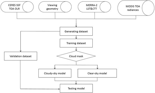
After applying these criteria, a training dataset containing 2,189,268 samples was established from coincident MODIS observations and the CERES TOA OLR product from four months in 2007. In the training dataset, CERES TOA OLR are taken as labels while the MODIS radiances are taken as input features. The dataset was randomly stratified into two groups, where 90% was used for the training dataset and the remaining 10% formed the testing dataset. Finally, models were built based on the training dataset with the cloud masks using the GBRT method.

GBRT, an advanced statistical model, has been widely used in both classification and prediction. As it does not require assumptions on the training dataset, it can deal with the uneven distribution of data attributes. In addition to the lack of limitation for any hypothesis of input data, the extensive usage of GBRT method also attributes to its better predictive capacity than a single decision tree and its ability to deal with data with huge size. The basic idea of the GBRT model is generating a strong classifier by constructing M amount of different weak classifiers through multiple iterations. Each iteration is used to improve the previous result by reducing the residuals of the previous model and establishing a new combination model in the gradient direction (Friedman 2001). Using this model, we obtained clear-sky and cloudy-sky models for TOA OLR estimation. The former was defined as no cloud coverage, while conditions with cloud fractions larger than 0% were used for the latter. If the pixel is partially cloudy or partially clear, it would also be identified as ‘cloudy pixel’.

4. Results and analysis

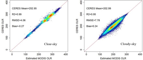
The inputs for the machine learning model used in this study included MODIS TOA radiance (channels 20–25 and 27–36), VZA, and MERRA-2 (land surface temperature, and cloud-top temperature), while the CERES SSF TOA OLR products were taken as ‘true values’. The test global results from 4 months in 2007 obtained via the GBRT method are shown in Figure 2. The root mean square errors (RMSEs) of the GBRT results under the clear-sky and cloudy-sky conditions are 4.06 W/m² and 7.78 W/m², while the biases are −0.27 W/m² and 0.24 W/m², respectively. The sample number of clear-sky condition (762,665) is much less than that of cloudy-sky condition (1,426,603). The high-density values of the clear-sky condition are around 270 W/m², while they are around 200 W/m² under the cloudy-sky condition. This is due to the low cloud-top temperatures under the cloudy-sky condition.

Figure 2. Test results of the TOA OLR derived from the clear-sky and cloudy-sky models using GBRT (unit: W/m²).

As many variables are used for model training, it is necessary to analyze the contribution of each to the final output; the corresponding results are shown in Figure 3. For the clear-sky condition, bands 32, 31, and 33 account for over 90% of the total contribution. This makes sense because bands 31 and 32 are window channels (8–12 μm), through which more surface signals can reach the sensor. The primary use of band 33 is to retrieve temperature profiles, which explains its high relative importance. For the cloudy-sky condition, band 32 alone accounts for more than 50% of the contributions. Bands 33 and 31 make the next highest contributions after band 32 with percentages of 20% and 18%, respectively.

Figure 3. Relative importance of the 17 variables in the training process.

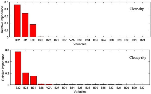
Although the relative importance of the other variables is very small, they cannot be omitted from the training process. To further illustrate this point, we reconduct the training process, and this time only top five channels shown in Figure 3 are used. The results show the training accuracy in both clear-sky and cloudy-sky condition become lower when the less important variables are removed. Specifically, the RMSE has increased from 4.06 W/m² to 4.39 W/m² for the clear-sky model, and for cloudy-sky model, it has increased from 7.78 W/m² to 8.42 W/m². As for the bias, however, it has a slight decrease. Overall, the removed bands are necessary in the training process. Thus, we still use all the 16 TIR bands in this study.

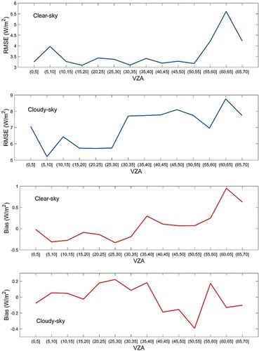
To further improve the retrieval accuracy, the VZA range was set to 0 to 70° with 5° intervals (i.e. 0–5°, 5°–10°, 10°–15°, … , 65°–70°). Machine learning models were then built separately in each VZA bin. Figure 4 shows the RMSE and bias of the test results in each group. For the clear-sky condition, the RMSEs are mostly less than 4 W/m² when the VZAs are smaller than 55°, and become much larger for groups with larger VZAs. The bias values mostly change between −0.5 W/m² and 0.5 W/m², except for the VZAs larger than 60°. For the cloudy-sky condition, the RMSEs range from 5 W/m² to 9 W/m² and also increase as the VZAs become larger. The Bias values are lower than those under the clear-sky condition, ranging from −0.4 W/m² to 0.2 W/m². Overall, after dividing the VZAs into these groups, the model performance became much better.

Figure 4. RMSE and Bias of the established models under the different VZA bins.

Compared to the instantaneous OLR, daily OLR is more useful in analyzing the Earth’s energy budget. Therefore, we developed real-time conversion ratios from CERES data to convert the instantaneous OLR to daily results. Specifically, the real-time conversion ratios are derived from CERES SYN daily and hourly data. Ratios of each hour are obtained by dividing CERES SYN1deg daily data by the corresponding CERES SYN1deg hourly data, and the ratio at the observation time is obtained by linear interpolation. Thus, daily OLR can be converted from instantaneous OLR using the following equation: (1) ${\mathrm{F}}_{OLR}^{daily}=r{\ast \mathrm{F}}_{OLR}^{instan}(t)$(1) where ${\mathrm{F}}_{OLR}^{daily}$ is the MODIS daily OLR, and the ${\mathrm{F}}_{OLR}^{instan}(t)$ is the instantaneous OLR at the observation time. $r$ is the derived conversion ratios.

The CERES TOA OLR is used as a baseline with which to compare the estimated MODIS OLR. Figure 5 shows an example of the high-resolution (1-km) OLR map in East Asia estimated from MODIS imagery, and the corresponding CERES OLR map is also presented for comparison. The overall patterns of the two OLR maps are quite similar, with much higher values in the tropics. However, the high-resolution MODIS OLR map shows more spatial details, which are essential for the study of local weather events or convective lifecycles. Figure 6 shows the spatial distribution and histogram of the differences between the two maps at 1° spatial resolution. We have converted the data into an equal area projection when calculating the regional mean OLR. Notable biases are found around Tibetan Plateau (also shown in Figure 7(c)), due to its unique climatic characteristics. The result indicates that the RMSE of the estimated MODIS OLR is 8.90 W/m², and the bias is 3.10 W/m². However, it is worth noting that for long-term monitoring study, this dataset cannot resolve any change less than 8.9 W/m², while CERES data could resolve.

Figure 5. CERES SYN and the estimated MODIS daily OLR in East Asia on January 1st, 2001.

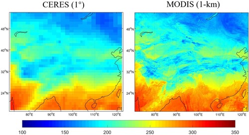
Figure 6. Spatial distribution and histogram of the differences between the estimated MODIS and CERES OLR in East Asia on January 1st, 2001.

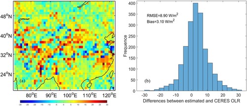
Figure 7. CERES monthly TOA OLR values and the differences from the estimated MODIS TOA OLR in January 2014 (a) CERES monthly TOA OLR (c) differences between estimated values and CERES, (b) and (d) are the same but for July 2014, (e) and (f) show corresponding total precipitable water vapor in MERRA-2.

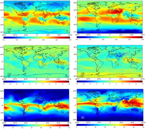
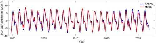
Compared to the daily TOA OLR, monthly products are more widely used when analyzing the long-term changes of the earth’s energy budget. Thus, monthly results are obtained by averaging the daily results. CERES monthly TOA OLR values and the differences from the estimated MODIS TOA OLR in January and July 2014 are shown in Figure 7. In January and July, there is no sunlight in the Arctic and Antarctica, respectively. Therefore, the temperature and the TOA OLR are much lower, as shown in Figure 7(a) and (b). Overall, the differences between the estimated MODIS TOA OLR and CERES monthly TOA OLR are quite small. Relatively larger differences are found in Tibetan Plateau and Intertropical Convergence Zone (ITCZ) in both months. In July 2014, obvious differences are also shown in the west of the America, the West Asia, and the Antarctica (Figure 7(c) and (d)). Considering that the OLR variations can be induced by water vapor (Huang, Ramaswamy, and Soden 2007; Sohn and Schmetz 2004), Figure 7(e) and (f) show the corresponding total precipitable water vapor in MERRA-2. The regional positive OLR biases (around the equator) in Figure 7(c) and (d) may partly attribute to the large total precipitable water vapor, as their similar spatial patterns can be seen, particularly in July (Figure 7(d) and (f)). Figure 8 shows the time series (2000–2021) results of the CERES and MODIS global land monthly mean TOA OLR anomalies. Overall, good consistency is shown between MODIS and CERES OLR, while small discrepancies are found after the year 2016.

Figure 8. Time series (2000–2021) results of the CERES and MODIS global land monthly mean TOA OLR anomalies.

5. Conclusions

The TOA OLR is a key component of the Earth’s energy budget, and numerous TOA OLR products have been developed from data acquired by broadband and narrowband satellite sensors. This study presented a companion work to our recent research in which a robust machine learning based method for estimating TOA albedos was proposed based on AVHRR data (Zhan and Liang 2022). As the quality of MODIS data is much better than that of AVHRR data, we chose to retrieve TOA OLR from MODIS data using a similar method in this study.

We used the direct estimation method, the essence of which was to estimate the TOA OLR from spectral information by establishing a relationship between the MODIS TOA radiances and TOA OLR. A widely used machine learning method (i.e. GBRT) was used for model building. The CERES SSF TOA OLR product was taken as the ‘true values’, and cloud masks were used to build clear-sky and cloudy-sky models separately. The test results showed that the RMSEs of the clear-sky and cloudy-sky models were 4.1 and 7.8 W/m², respectively.

As daily OLR is more commonly used in analyzing the Earth’s energy budget, we converted the estimated instantaneous OLR to daily results using real-time conversion ratios derived from CERES daily and hourly OLR data. Comparison results showed the RMSE of the estimated MODIS OLR was 8.9 W/m² in East Asia. The proposed TOA OLR retrieval algorithm is robust, and the developed dataset using the algorithm will be the first high resolution (1-km) OLR product.

Overall, we consider the quality of the MODIS TOA OLR retrievals to be ‘good’ after comparing them with CERES datasets, especially for the monthly results. The reported daily bias of Yadav, Giri, and Bhan (2022) is ±5–6 W/m² when taken CERES data as reference. However, the spatial resolution of their product is relatively coarse (10-km) and the spatial extent is also limited (ranging over 40°N–40°S & 35°E–135°E). The reported daily bias and standard deviation of Wang et al. (2021) are ±0.6 W/m² and 4.88–9.1 W/m² respectively, which are comparable with this study. We believe the high resolution (1-km) MODIS TOA OLR dataset can provide benefits for researchers as well as the repository of data, especially for the research at regional scales. However, there are still room for improvements. For example, in the future work training models could be built for each scene type, and the criteria set to collect MODIS-CERES data pairs could be further adjusted.

Acknowledgements

We thank for the data support from ‘National Earth System Science Data Center, National Science & Technology Infrastructure of China’ (http://www.geodata.cn). We would like to thank the anonymous reviewers for their constructive comments and suggestions.

Disclosure statement

No potential conflict of interest was reported by the author(s).

Data availability

The CERES datasets are downloaded at https://ceres-tool.larc.nasa.gov/ord-tool/jsp/SYN1degEd4Selection.jsp. The MODIS data are downloaded at https://modis.gsfc.nasa.gov/, and the MERRA-2 data can be downloaded at https://gmao.gsfc.nasa.gov/reanalysis/merra-2.

Additional information

Funding

This study was supported by the Open Research Program of the International Research Center of Big Data for Sustainable Development Goals (grant no. CBAS2022ORP01) and the National Natural Science Foundation of China (grant no. 42090011).

References

- Ba, Mamoudou B, Robert G Ellingson, and A. Gruber. 2003. “Validation of a Technique for Estimating OLR with the GOES Sounder.” Journal of Atmospheric and Oceanic Technology 20 (1): 79–89. doi:10.1175/1520-0426(2003)020<0079:VOATFE>2.0.CO;2
- Barkstrom, Bruce R. 1984. “The Earth Radiation Budget Experiment (ERBE).” Bulletin of the American Meteorological Society 65 (11): 1170–1185. doi:10.1175/1520-0477(1984)065<1170:TERBE>2.0.CO;2
- Barnes, William L, Thomas S Pagano, and Vincent V Salomonson. 1998. “Prelaunch Characteristics of the Moderate Resolution Imaging Spectroradiometer (MODIS) on EOS-AM1.” IEEE Transactions on Geoscience and Remote Sensing 36 (4): 1088–1100. doi:10.1109/36.700993
- Chu, Pao-Shin, and Jian-Bo Wang. 1997. “Recent Climate Change in the Tropical Western Pacific and Indian Ocean Regions as Detected by Outgoing Longwave Radiation Records.” Journal of Climate 10 (4): 636–646. doi:10.1175/1520-0442(1997)010<0636:RCCITT>2.0.CO;2
- Doelling, David R, Norman G Loeb, Dennis F Keyes, Michele L Nordeen, Daniel Morstad, Cathy Nguyen, Bruce A Wielicki, David F Young, and Moguo Sun. 2013. “Geostationary Enhanced Temporal Interpolation for CERES Flux Products.” Journal of Atmospheric and Oceanic Technology 30 (6): 1072–1090. doi:10.1175/JTECH-D-12-00136.1
- Friedman, Jerome H. 2001. “Greedy Function Approximation: A Gradient Boosting Machine.” Annals of Statistics 29 (5): 1189–1232. doi:10.1214/aos/1013203451
- Harries, John E, J. E. Russell, J. A. Hanafin, H. Brindley, J. Futyan, J. Rufus, S. Kellock, G. Matthews, R. Wrigley, and A. Last. 2005. “The Geostationary Earth Radiation Budget Project.” Bulletin of the American Meteorological Society 86 (7): 945–960. doi:10.1175/BAMS-86-7-945
- Huang, Yi, V. Ramaswamy, and Brian Soden. 2007. “An Investigation of the Sensitivity of the Clear-Sky Outgoing Longwave Radiation to Atmospheric Temperature and Water Vapor.” Journal of Geophysical Research: Atmospheres 112: D5. doi:10.1029/2006JC003735
- Kandel, R., M. Viollier, P. Raberanto, J. Ph Duvel, L. A. Pakhomov, V. A. Golovko, A. P. Trishchenko, J. Mueller, E. Raschke, and R. Stuhlmann. 1998. “The ScaRaB Earth Radiation Budget Dataset.” Bulletin of the American Meteorological Society 79 (5): 765–784. doi:10.1175/1520-0477(1998)079<0765:TSERBD>2.0.CO;2
- Kim, Bu-Yo, Kyu-Tae Lee, Joon-Bum Jee, and Il-Sung Zo. 2018. “Retrieval of Outgoing Longwave Radiation at Top-of-Atmosphere Using Himawari-8 AHI Data.” Remote Sensing of Environment 204: 498–508. doi:10.1016/j.rse.2017.10.006
- Lee, Hai-Tien, Arnold Gruber, Robert G Ellingson, and Istvan Laszlo. 2007. “Development of the HIRS Outgoing Longwave Radiation Climate Dataset.” Journal of Atmospheric and Oceanic Technology 24 (12): 2029–2047. doi:10.1175/2007JTECHA989.1
- Lee, Thomas F, J. D. Hawkins, A. P. Kuciauskas, and S. D. Miller. 2010. Applications and Training for Next-Generation Imagers. Atlanta: American Meteorological Society.
- Liang, Shunlin, Dongdong Wang, Tao He, and Yunyue Yu. 2019. “Remote Sensing of Earth’s Energy Budget: Synthesis and Review.” International Journal of Digital Earth 12 (7): 737–780. doi:10.1080/17538947.2019.1597189
- Liu, Xiangyang, Bo-Hui Tang, Guangjian Yan, Zhao-Liang Li, and Shunlin Liang. 2019. “Retrieval of Global Orbit Drift Corrected Land Surface Temperature from Long-Term AVHRR Data.” Remote Sensing 11 (23): 2843. doi:10.3390/rs11232843
- Nitta, Tsuyoshi, and Shingo Yamada. 1989. “Recent Warming of Tropical Sea Surface Temperature and its Relationship to the Northern Hemisphere Circulation.” Journal of the Meteorological Society of Japan. Ser. II 67 (3): 375–383. doi:10.2151/jmsj1965.67.3_375
- Park, Myung-Sook, Chang-Hoi Ho, Heeje Cho, and Yong-Sang Choi. 2015. “Retrieval of Outgoing Longwave Radiation from COMS Narrowband Infrared Imagery.” Advances in Atmospheric Sciences 32 (3): 375–388. doi:10.1007/s00376-014-4013-7
- Rienecker, M. M., M. J. Suarez, R. Gelaro, R. Todling, J. Bacmeister, E. Liu, M. G. Bosilovich, S. D. Schubert, L. Takacs, and G. K. Kim. 2011. “MERRA: NASA’s Modern-Era Retrospective Analysis for Research and Applications.” Journal of Climate 24 (14): 3624–3648. doi:10.1175/JCLI-D-11-00015.1
- Schmetz, Johannes, and Quanhua Liu. 1988. “Outgoing Longwave Radiation and its Diurnal Variation at Regional Scales Derived from Meteosat.” Journal of Geophysical Research: Atmospheres 93 (D9): 11192–11204. doi:10.1029/JD093iD09p11192
- Sohn, Byung-Ju, and Johannes Schmetz. 2004. “Water Vapor–Induced OLR Variations Associated with High Cloud Changes Over the Tropics: A Study from Meteosat-5 Observations.” Journal of Climate 17 (10): 1987–1996. doi:10.1175/1520-0442(2004)017<1987:WVOVAW>2.0.CO;2
- Wang, Dongdong, and Shunlin Liang. 2016. “Estimating High-Resolution Top of Atmosphere Albedo from Moderate Resolution Imaging Spectroradiometer Data.” Remote Sensing of Environment 178: 93–103. doi:10.1016/j.rse.2016.03.008
- Wang, Tianyuan, Lihang Zhou, Changyi Tan, Murty Divakarla, Ken Pryor, Juying Warner, Zigang Wei, Mitch Goldberg, and Nicholas R Nalli. 2021. “Validation of Near-Real-Time NOAA-20 CrIS Outgoing Longwave Radiation with Multi-Satellite Datasets on Broad Timescales.” Remote Sensing 13 (19): 3912. doi:10.3390/rs13193912
- Wargan, Krzysztof, and Lawrence Coy. 2016. “Strengthening of the Tropopause Inversion Layer During the 2009 Sudden Stratospheric Warming: A MERRA-2 Study.” Journal of the Atmospheric Sciences 73 (5): 1871–1887. doi:10.1175/JAS-D-15-0333.1
- Wielicki, Bruce A, Bruce R Barkstrom, Edwin F Harrison, Robert B Lee, G. Louis Smith, and John E Cooper. 1996. “Clouds and the Earth’s Radiant Energy System (CERES): An Earth Observing System Experiment.” Bulletin of the American Meteorological Society 77 (5): 853–868. doi:10.1175/1520-0477(1996)077<0853:CATERE>2.0.CO;2
- Yadav, Ramashray, R. K. Giri, and S. C. Bhan. 2022. “High-Resolution Outgoing Long Wave Radiation Data (2014–2020) of INSAT-3D Imager and its Comparison with Clouds and Earth’s Radiant Energy System (CERES) Data.” Advances in Space Research 70 (4): 976–991. doi:10.1016/j.asr.2022.05.053
- Zhan, Chuan, Richard P Allan, Shunlin Liang, Dongdong Wang, and Zhen Song. 2019. “Evaluation of Five Satellite Top-of-Atmosphere Albedo Products Over Land.” Remote Sensing 11 (24): 2919. doi:10.3390/rs11242919
- Zhan, Chuan, and Shunlin Liang. 2022. “Improved Estimation of the Global Top-of-Atmosphere Albedo from AVHRR Data.” Remote Sensing of Environment 269: 112836. doi:10.1016/j.rse.2021.112836