How the physical inactivity is affected by social-, economic- and physical-environmental factors: an exploratory study using the machine learning approach

ABSTRACT

Previous studies have utilized regression models to investigate the impact of environmental factors on physical activity. However, such approaches are inadequate for data-driven analysis seeking to identify robust associations from the intricate and multi-variable interactions between physical activity and environmental factors. With the emergence of the concept of the exposome, which encompasses the totality of exposures, this paper explores machine learning models for predicting the percentage of physical inactivity in U.S. counties, while considering 28 social-, economic-, and physical-environmental factors. The aim of this study is to address the research gap and gain insight into the complex associations between environmental exposures and physical activity. Five machine learning models were tested, and the performances were compared to select the best classifier for further investigation. This study used data from the Behavioral Risk Factor Surveillance System (BRFSS) of the Centers for Disease Control and Prevention. The mean population of all counties was 102,841, and the mean percentage of population below 18 years was 22.3%. The partial dependence plot analysis indicated that only one feature – bachelor’s degree – exhibited a close-to-linear relationship with physical inactivity. Motor-vehicle crash death rate and mean temperature showed nonlinear and non-monotonic relationships with the predicted percentage of physical inactivity.

KEYWORDS:

• Physical inactivity
• environmental effects
• machine learning
• GIS

1. Introduction

Physical inactivity has been identified as one of the top public health concerns, with approximately 27.5% of adults globally having insufficient levels of physical activity (Guthold et al. 2018; Katzmarzyk et al. 2022). Physical activity is defined as ‘any bodily movement produced by skeletal muscles that result in energy expenditure’ (Caspersen et al. 1985). It is recommended that adults should engage in 150–300 min of moderate or 75–150 min of vigorous physical activity per week (Piercy et al. 2018). Evidence shows that not meeting the guidelines for physical activity – physical inactivity – is associated with the prevalence of obesity and other chronic diseases, including cardiovascular diseases, type-2 diabetes, colon cancer, depression, and breast cancer (Bassuk and Manson 2005; Bull et al. 2004; Lee et al. 2012; Physical Activities Guidelines Advisory Committee 2018; Stein and Colditz 2004).

Understanding the motivation and mechanism of physical inactivity can help develop intervention strategies to improve public health. Research shows that changes in environmental contexts and built environments may affect health behaviors and enhance or limit the opportunities for physical activity (Brownson, Boehmer, and Luke 2005; Davison and Lawson 2006; Ferreira et al. 2007; Frank et al. 2005; McCormack et al. 2004; Saelens, Sallis, and Frank 2003; Sallis et al. 2009). Identifying the environmental contexts in which physical activity occurs can help identify ways to encourage physical activity by modifying those contexts (Houston 2014). The geographic information system (GIS) is an effective tool for spatially examining the effects of social-, economic-, and physical-environmental factors on physical inactivity (Almanza et al. 2012; Clary et al. 2020; da Silva et al. 2017; James et al. 2020; Jansen et al. 2016; Loh et al. 2019; Rodríguez et al. 2012; Troped et al. 2010).

However, existing studies have used multiple regression or logistic regression models to investigate the associations between physical activity and environmental factors (Almanza et al. 2012; Jansen et al. 2016). These statistical approaches are not suitable for data-driven analysis that seeks to find robust associations from the complicated and multi-variable interactions between physical activity and environmental factors. Statistical models generally require manageable datasets with smaller numbers of attributes (c.f., (Wang, Lee, and Kwan 2018)), and using many input variables can cause large standard errors with wide and imprecise confidence intervals (Ranganathan, Pramesh, and Aggarwal 2017). Using many independent variables in a regression model can also attenuate true associations or even result in spurious associations. With the emergence of the concept of the exposome as the totality of exposures (Wild 2012), recent studies in different fields, however, are attempting to consider more complete environmental factors, including general external factors (Eskola et al. 2020; Golding et al. 2014; Konstantinou et al. 2021; Loh et al. 2017), and consequently, many predictors derived from various environmental factors need to be considered together in a predictive model to examine the complex associations.

To address the research gap and gain a clear understanding of the relationship between various environmental exposures and physical activity, this study explores the use of machine learning models to predict the percentage of physical inactivity in U.S. counties. The prediction is based on a consideration of self-reported health status, social-, economic-, and physical-environmental factors, as well as demographic information from 2015 to 2018. Machine learning models are particularly useful in explaining the nonlinear associations that may exist between environmental factors and physical activity. In this study, five machine learning models were tested and compared, including Support Vector Regression (SVR), Decision Tree (DT), Random Forest (RF), eXtreme Gradient Boosting (XGB), and Multilayer Perceptron (MLP).

To further investigate the associations between important environmental factors and physical inactivity, this study also conducted partial dependence plots (PDPs) analysis. This method was used to understand the complicated interactions between different factors, including those that cannot be explored using linear regression. PDPs with a trained model are an effective way to investigate the nonlinearity of factors and address mixed or unexpected associations of certain factors, such as temperature, with physical activity (Brodersen et al. 2005). Previous studies have examined correlates of physical activity using data mining or machine learning techniques (Yoon, Suero-Tejeda, and Bakken 2015; Farrahi et al. 2020; Lakerveld et al. 2017). However, feature importance and nonlinear associations between various factors and physical activity have yet to be fully understood. Therefore, this study seeks to contribute to the existing literature by providing a more comprehensive understanding of these associations.

2. Materials and methods

2.1. Datasets

2.1.1. Physical inactivity data

The study utilized physical inactivity percentage data for U.S. counties between 2015 and 2018. The data were collected by the Behavioral Risk Factor Surveillance System (BRFSS) of the Centers for Disease Control and Prevention through telephone surveys. BRFSS is a cooperative project between the Robert Wood Johnson Foundation and the University of Wisconsin Population Health Institute, which conducts 400,000 adult interviews annually and aggregates the data for each state. In the data, physical inactivity represents the percentage of adults aged 20 and over who reported no leisure-time physical activity, such as running, calisthenics, golf, gardening, and brisk walking for exercise. Participants who responded ‘no’ to the question ‘During the past month, other than your regular job, did you participate in any physical activities or exercises such as running, calisthenics, golf, gardening, or walking for exercise?’ were considered physically inactive.

The descriptive statistics of 3078 counties in 2018 are presented in Table 1. The mean population of all counties was 102,841, with a mean percentage of the population below 18 years of 22.3%. Additionally, the mean percentage of population over 65 years was 18.4%, and the mean percentage of females was 49.9%.

Table 1. Descriptive statistics of 3,078 counties in 2018.

Measure	Min	Max	Mean	Standard deviation
Population	88	10,137,915	102,841	330,319
% below 18 years of age	0.0	40.8	22.3	3.5
% 65 and older	4.6	56.3	18.4	4.6
% Non-Hispanic African American	0.0	85.2	8.9	14.3
% American Indian and Alaskan Native	0.0	93.1	2.3	7.7
% Asian	0.0	44.3	1.5	2.9
% Native Hawaiian/Other Pacific Islander	0.0	50.0	0.1	1.0
% Hispanic	0.5	96.3	9.3	13.7
% Non-Hispanic white	2.8	98.0	76.6	20.1
% Females	27.8	56.5	49.9	2.3

2.1.2. Feature extraction

Physical-Environmental Factors: Out of the 28 factors considered in this study, 12 factors were chosen for physical environments. Unnecessary features, which could be substituted by another representative measure or feature (e.g. mean temperature, minimum temperature, and maximum temperature), were excluded based on correlation analysis (Pearson correlation coefficients larger than 0.8). All the included physical-environmental factors are listed and described in Table 2. According to previous physical activity research, the factors in the physical environment should include harmful substances, like air pollution, access to various health-related resources, like recreational resources, and community design and built environment (Council and Population 2013). Thus, this study selected access to exercise opportunities, air pollution (PM2.5), elevation, food environment, land-cover types, motor-vehicle crash death rates, severe housing problems, slope, precipitation, temperature, and tree canopy as the physical environmental factors, which have been widely used in previous studies (An et al. 2019; Davison and Lawson 2006; van Stralen et al. 2009). It is worth noting that some of these factors, such as access to exercise opportunities, precipitation, slope, temperature, and traffic crashes, were found to have inconsistent outcomes or no association with physical activity in previous studies (Humpel 2002; McGinn et al. 2007). There are available data for all physical environmental factors from 2015 to 2018 except for elevation, land-cover types, slope, and tree canopy. Specifically, the land-cover types and tree canopy for 2015 were calculated using 2013 data, while 2016–2018 land-cover types and tree canopy were based on 2016 data. Figure 1 illustrates the mean slope as an example of the physical environmental factors.

Social- and Economic-Environmental Factors and Self-reported health status: County-level social- and economic-environmental factors, including demographic characteristics and socio-economic status, were mostly derived from the 2015–2018 American Community Survey (ACS) data. Of the 2,034 variables in the ACS data, 13 social- and economic-environmental variables, including demographic and socio-economic factors potentially associated with physical inactivity, were selected (Table 3). These variables were also used in a previous study (Wang, Lee, and Kwan 2018) because most of the variables, including age, sex, employment, income, occupation, race, and vehicle ownership, were significantly associated with physical inactivity. These social and economic features of the counties are also diverse. For instance, the unemployment rate varies from 0 to 18%, covering counties without any unemployment problems and counties with significant unemployment problems. Median income ranges from about $7,000 to $60,000, which includes poor and rich counties. Population composition of the counties varies considerably regarding age (from youngsters to senior-dominated counties), gender, and race (e.g. from white to African American-dominated counties). The significant variation of social and economic environmental factors provides rich information for predicting physical inactivity and understanding the environmental effects on physical inactivity. Additionally, three other features possibly affecting physical activity – bachelor’s degree, social association rates, and violent crime rates – are also included in the analysis (Addy et al. 2004; Trost et al. 2002). Figure 2 illustrates the median income per capita as an example of the social and economic environmental factors. Fair or poor health is self-reported health status and an important factor that was found to be positively associated with physical activity (Trost et al. 2002). All of the social- and economic-environmental factors and self-reported health status were derived from the data collected in 2015–2018.

Figure 1. Physical environmental factor: mean slope (degree).

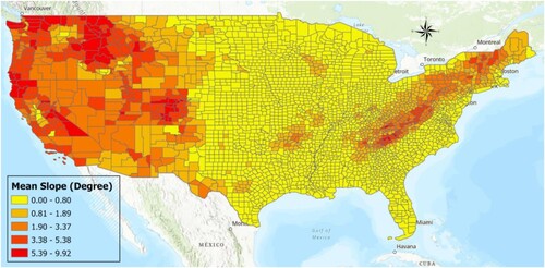
Figure 2. Social-environmental factor: median income per capita (in US Dollars).

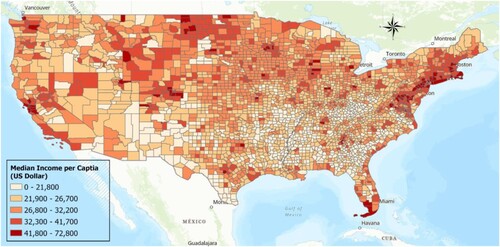
Table 2. Details of physical-environmental predictors.

	Name		Description	Data and years	Mean ± SD
Physical environment	Access to exercise opportunities (%)		Percentage of population with adequate access to locations for physical activity	BRFSS 2015–2018	61.4 ± 23.9
	Daily average PM 2.5 (days)		Annual number of unhealthy air quality days due to fine particulate matter	BRFSS 2015–2018	10.4 ± 2.0
	Elevation (m)		Mean digital elevation model value	Shuttle Radar Topography Mission v 4.1	440.2 ± 509.8
	Food environment index		Index of factors that contribute to a healthy food environment, 0 (worst) to 10 (best)	2015–2018	7.1 ± 1.2
	Land cover	Open space (%)	Density of land cover 21. Areas with a mixture of some constructed materials, but mostly vegetation in the form of lawn grasses. Large-lot single-family housing units, parks, golf courses, and vegetation planted in developed settings for recreation, erosion control, or aesthetic purposes	Multi-Resolution Land Characteristics (MRLC) Consortium 2013 data for 2015, 2016 data for 2016–2018	4.8 ± 4.1
		Highly developed (%)	Density of land cover24. Areas where people reside or work in large numbers. Apartment complexes, row houses and commercial/industrial buildings	MRLC Consortium 2013 data for 2015, 2016 data for 2016–2018	0.6 ± 2.7
	Motor-vehicle crash death rate (cases per 100,000)		Number of deaths due to traffic accidents involving a motor vehicle per 100,000 population	BRFSS 2015–2018	17.0 ± 10.9
	Severe housing problems (%)		Percentage of households with at least 1 of 4 housing problems: overcrowding, high housing costs, or lack of kitchen or plumbing facilities	BRFSS 2015–2018	14.4 ± 4.4
	Slope (°)		Mean slope	Shuttle Radar Topography Mission v 4.1	1.0 ± 1.3
	Precipitation (mm)		Annual-based measure for mean precipitation	PRISM Climate Group 2015–2018	1125.1 ± 440.3
	Temperature (°C)		Annual-based measures for mean temperature	PRISM Climate Group 2015–2018	13.2 ± 4.6
	Tree canopy (%)		Annual-based measure for mean canopy size	US Forest Service 2013 data for 2015, 2016 data for 2016–2018	29.6 ± 24.5

Table 3. Details of social- and economic-environmental predictors.

	Name		Description	Data and years	Mean ± SD
Social and economic environment	Age		Median age	American Community Survey (ACS) 2015–2018	41.0 ± 5.3
	Crime		Violent crime rate	BRFSS 2015–2018	238.6 ± 196.0
	Education attainment (%)		Percentage of residents who have bachelor’s degree	ACS 2015–2018	13.8 ± 5.6
	Employment		Unemployment rate	ACS 2015–2018	3.8 ± 1.6
	Home ownership (%)		Percentage of housing units that are owner-occupied	ACS 2015–2018	58.2 ± 9.2
	Income ($)		Income per capita (inflation-adjusted dollars)	ACS 2015–2018	23659.2 ± 8101.2
	Occupation	Natural resources, construction or maintenance (%)	Percentage of residents whose occupations are natural resources, construction or maintenance	ACS 2015–2018	12.6 ± 4.2
		Production, transportation or material moving (%)	Percentage of residents whose occupations are production, transportation or material moving	ACS 2015–2018	16.1 ± 5.8
	Poor or fair health (%)		Percentage of adults reporting fair or poor health (age-adjusted)	BRFSS 2015–2018	16.6 ± 5.9
	Race	African American (%)	Percentage of residents who are African American	ACS 2015–2018	9.1 ± 14.3
		Asian (%)	Percentage of residents who are Asian	ACS 2015–2018	1.3 ± 2.3
		Hispanic (%)	Percentage of residents who are Hispanic and Latino	ACS 2015–2018	9.4 ± 13.9
	Self-employed unpaid family workers (%)		Percentage of residents who are self-employed unpaid family workers	ACS 2015–2018	8.0 ± 3.9
	Sex (%)		Percentage of residents who are female	ACS 2015–2018	50.0 ± 2.3
	Social association		Social association rate	BRFSS 2015–2018	13.8 ± 6.9
	Vehicle ownership (%)		Percentage of families who have no vehicles available	ACS 2015–2018	6.3 ± 3.7

2.2. Machine learning models

In this study, we investigated various machine learning models to predict physical inactivity percentages in U.S. counties based on social-, economic-, and physical-environmental factors. Machine learning models have the capability to handle a larger number of input variables than traditional statistical models (Sheojung et al. 2021). Our approach considers not only socio-demographic factors but also GIS-based environmental factors in predicting physical inactivity percentages at the county level. We used five models for this study, namely Support Vector Regression (SVR), Decision Tree (DT), Random Forest (RF), eXtreme Gradient Boosting (XGB), and Multilayer Perceptron (MLP). The training, testing, and evaluation of these models were implemented using the Python programming language (version 3.9) and Scikit-learn library (version 0.24) (Pedregosa et al. 2018).

To optimize the performance of each model, hyper-parameter calibration was performed using an exhaustive grid search. Table 4 shows the hyper-parameter ranges for tuning SVR, DT, RF, XGB, and MLP, along with the corresponding optimized hyper-parameter combinations. The exhaustive grid search attempted all possible combinations of hyper-parameter values to find the one with the highest mean accuracy based on three-fold cross-validation. Each year of data from 2015 to 2018 and the entire four-year data were tested.

Table 4. Hyper-parameter ranges and optimized hyper-parameter combinations.

Hyper-parameter ranges for tuning	SVR	kernel $\in$ [‘linear’, ‘poly’, ‘rbf’, ‘sigmoid’], C $\in$ [0.001, 0.01, 0.1, 1, 10], gamma $\in$ [0.001, 0.01, 0.1, 1], epsilon $\in$ [0.001, 0.01, 0.1, 1]
	DT	maximum depth $\in$[5, 10, 20, 30], minimum samples leaf $\in$ [1, 2, 3], minimum samples split $\in$ [7, 10, 13]
	RF	maximum depth $\in$ [5, 10, 20, 30], minimum samples leaf $\in$ [1, 2, 3], minimum samples split $\in$ [7, 10, 13], number of estimators $\in$ [1000, 1500, 2000]
	XGB	learning rate $\in$ [0.01, 1], subsample $\in$ [0.8, 1.0], subsample ratio of columns for each tree $\in$ [0.8, 1.0], maximum depth $\in$ [5, 10, 20, 30], number of estimators $\in$ [1000, 1500, 2000]
	MLP	hidden layer sizes $\in$ [(50,50,50), (50,100,50), (150,100,50), (100,)], activation $\in$ [‘tanh’, ‘relu’], solver $\in$ [‘sgd’, ‘adam’], alpha $\in$ [0.0001, 0.05], learning rate $\in$ [‘constant’, ‘adaptive’]
Optimized hyper-parameter combination	SVR	kernel = [‘rbf'’], C = 10, gamma = 0.001, epsilon = 0.1
	DT	maximum depth = 10, minimum samples leaf = 3, minimum samples split = 13
	RF	maximum depth = 30, minimum samples leaf = 1, minimum samples split = 7, number of estimators = 1500
	XGB	learning rate = 0.01, subsample = 0.8, subsample ratio of columns for each tree = 0.8, maximum depth = 10, number of estimators = 2000
	MLP	hidden layer sizes = (100,), activation = ‘relu’, solver = ‘adam’, alpha = 0.05, learning rate = ‘adaptive’

In evaluating the performance of the models, we used pseudo R-squared, mean squared error (MSE), root mean squared error (RMSE), and mean absolute error (MAE) as measures of model fit. R-squared represents the proportion of the variance of the dependent variable that is explained by the independent variables. MSE is the average of the squared difference between the original and predicted values, and it measures the variance of the residuals. RMSE represents the square root of MSE and measures the standard deviation of residuals. MAE is a measure of the average absolute difference between predicted and actual values and measures the average of the residuals. They were estimated with 10-fold cross-validation after the tuning process in order to compare and evaluate the performances of the models and determine the best model for further investigation.

Finally, we examined the associations between selected variables and physical inactivity percentages using PDPs, which allowed us to explore the associations focusing on directions and linearity and show the average marginal effect that one or two features have on the predicted outcome (Friedman 2001). Therefore, they can be used to explore whether the association of a specific variable is linear, monotonic, or more complex.

3. Results

3.1. Percentage of physical inactivity

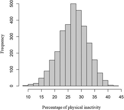
As for the physical inactivity data, the percentage ranges from about 9–43% among U.S. counties. Figure 3 illustrates the physical inactivity percentages follow a standard distribution with short tails. The average percentage of physical activity is 27%, with a standard deviation of 5%.

Figure 3. Distribution of percentage of physical inactivity among U.S. counties.

3.2. Prediction performance

In this section, we report the evaluation results obtained with the different models. Table 5 demonstrates the model fit measures of the five models calculated based on 10-fold cross-validation. 2015, 2016, 2017, 2018, and the whole four-year data were used for training models specifically. As a result, the best model fit (highest R² and lowest MSE, RMSE and MAE; see the bold fonts in Table 5) was achieved by XGB with tuned hyperparameters (see Table 4 for details on the parameters) for all of the datasets in the different years. It was slightly better than RF. MLP and SVR showed relatively moderate results when compared with RF and XGB. DT, however, achieved the worst prediction performance among the five models. The best algorithm, XGB, was also compared with the others using Finner’s method, which is one of the most powerful 1:N post-hoc analyses (Santafe, Inza, and Lozano 2015). Based on the results of the RMSE or MAE using 2015, 2016, 2017, and 2018 datasets, the adjusted p-values less than 0.05 (see Table 6) represent significant differences from the best model, XGB. Comparing the RMSE, SVR and RF were not significantly different from XGB, while DT and MLP were significantly different (p < 0.05; bold fonts in Table 6). Regarding the MAE, only DT was significantly different from XGB. As a result, XGB was chosen as the best model for further analysis.

Table 5. Comparison of performances of five machine learning models.

		SVR	DT	RF	XGB	MLP
2015	R^2	0.69	0.58	0.76	0.78	0.70
	MSE	8.59	11.83	6.77	6.31	8.34
	RMSE	2.93	3.44	2.60	2.51	2.89
	MAE	2.33	2.68	2.05	1.98	2.26
2016	R^2	0.72	0.59	0.76	0.77	0.70
	MSE	8.13	12.07	7.13	6.61	8.60
	RMSE	2.85	3.47	2.67	2.57	2.93
	MAE	2.26	2.73	2.10	2.01	2.31
2017	R^2	0.72	0.54	0.74	0.75	0.71
	MSE	7.37	12.04	6.75	6.41	7.46
	RMSE	2.71	3.47	2.60	2.53	2.73
	MAE	2.13	2.73	2.06	1.99	2.14
2018	R^2	0.69	0.54	0.73	0.75	0.68
	MSE	8.32	12.20	7.05	6.67	8.37
	RMSE	2.88	3.49	2.65	2.58	2.89
	MAE	2.28	2.75	2.11	2.03	2.25
All	R^2	0.70	0.69	0.84	0.86	0.78
	MSE	8.37	8.72	4.42	3.98	6.07
	RMSE	2.89	2.95	2.10	1.99	2.46
	MAE	2.29	2.27	1.63	1.55	1.93

Table 6. 1:N performance comparisons using Finner’s method (adjusted p-values).

	SVR	DT	RF	XGB	MLP
RMSE	0.058	0.001	0.371	–	0.028
MAE	0.050	0.001	0.371	–	0.050

Figure 4 shows the spatial distribution of the physical inactivity percentages in 2018, and Figure 5 illustrates the spatial distribution of prediction error in percentage for the best-performing XGB model with 2018 data. 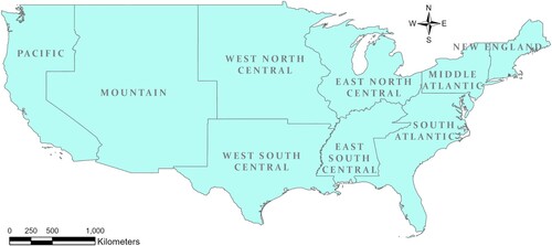The percentage prediction error was calculated with the formula (1): (1) $\mathrm{Percentage}\mathrm{prediction}\mathrm{error}={\displaystyle \frac{(\mathrm{Predicted}\mathrm{physical}\mathrm{inactivity}\mathrm{rate}\text{-}\mathrm{measured}\mathrm{physical}\mathrm{inactivity}\mathrm{rate})}{\mathrm{measured}\mathrm{physical}\mathrm{inactivity}\mathrm{rate}}}$(1) In Figure 5, the color shades and volume heights represent the percentage differences between the predicted and measured values. Red colors indicate positive values, while blue colors represent negative values. The negative value indicates that the prediction is lower than the actual physical inactivity level, while the positive value indicates that the prediction is higher than the actual physical inactivity level. The counties in the Pacific and South Atlantic had mostly positive prediction errors. In contrast, the Mountain area, West South Central, East South Central, Middle Atlantic, and New England mostly showed negative prediction errors. At the same time, the West North Central and East North Central demonstrated mixed error patterns (see Figure 6 for main divisions of United States).

Figure 4. Spatial distribution of physical inactivity percentages in 2018.

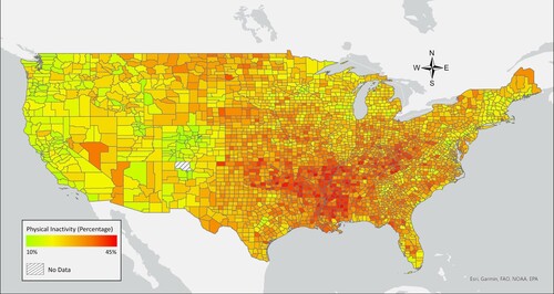
Figure 5. Spatial distribution of prediction error in percentage for the best performed extreme gradient boosting prediction model.

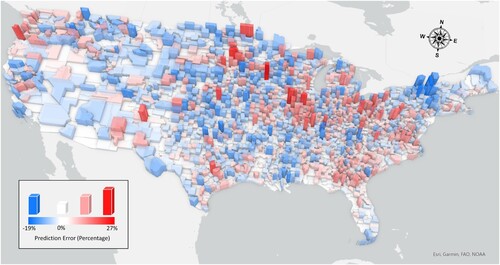
Figure 6. Map of main divisions of United States.

We further examined when the negative or positive prediction errors occurred. As shown in Figure 7, none of the top five important prediction features (Figure 8 (a)) had any pattern associated with predicted physical inactivity. However, the measured physical inactivity contributed to the separation of negative and positive prediction errors. Compared with the positive prediction errors, high negative prediction errors were associated more with the counties that had higher measured physical inactivity. This implies that XGB predicted physical inactivity conservatively for the counties having top 50 negative or positive prediction errors, and did not vary much in the middle range of measured physical inactivity percentages.

Figure 7. Parallel coordinate plot for the counties having top 50 positive or negative prediction errors. PI: physical inactivity percentage; BACHEL: bachelor’s degree; Fair_Poor: fair/poor health; SLOPE: slope; HISP: Hispanic population; TEMPMEAN: mean temperature.

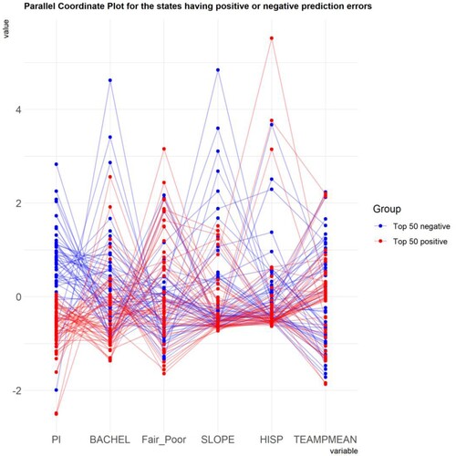
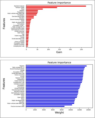
Figure 8. Importance of features for eXtreme Gradient Boosting model. Occupation: PTMM: occupation: production, transportation, and material moving; Occupation: NRCM: occupation: natural resources, construction, and maintenance. (a) Gain importance; (b) Weight importance.

3.3. Importance of features and partial dependence plots analysis

The XGB prediction model, the best-performing model, can analyze the relative importance of predictors. Feature importance is a critical result of XGB, which can help understand how important each feature is in predicting the outcome. Figure 8 (a) and (b) plot the relative importance of features with gain importance and weight importance using the 2015–2018 data. Gain importance is the average gain across all splits in each tree where the corresponding feature was used. Weight importance, on the other hand, is the number of times the corresponding feature is used to split data in each tree. Features are ordered top-to-bottom as most to least important.

It can be seen from the figure that bachelor’s degree, fair/poor health, and slope were the top three most important environmental variables in the gain importance. One of them was a physical-environmental factor, and two of them were social- and economic-environmental factors. In terms of weight importance, the Hispanic population, average daily PM2.5, and severe housing problems were found to be important. Compared with the gain importance, the top three important features in the weight importance were completely different. The top three important features – bachelor’s degree, fair/poor health, and slope – were found to be ranked in the middle or low in weight importance.

We explored the PDPs of the six important features in terms of gain importance, which had not been investigated in previous studies in terms of the associations between physical inactivity and environmental factors. The results of PDPs analysis of the six features are shown in Figure 9. Only one feature – bachelor’s degree – was close to linear, while fair/poor health, access to exercise opportunities, and slope were monotonic. Motor-vehicle crash death rate and mean temperature had nonlinear and non-monotonic relationships, respectively, with the predicted physical inactivity percentages.

Figure 9. Partial dependence plots of fair/poor health, access to exercise opportunities, motor-vehicle crash death rate, bachelor’s degree, mean temperature, and slope for physical inactivity percentage prediction. The ticks on the x-axis indicate the data distribution.

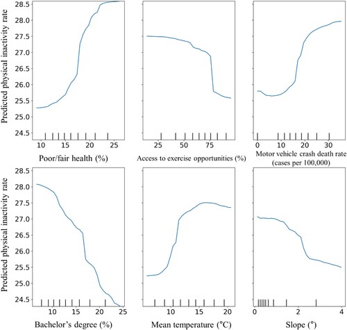
Fair/poor health showed a positive relationship with the predicted physical inactivity percentages. The more that adults reported fair or poor health, the higher the physical inactivity was. In terms of access to exercise opportunities, the predicted physical inactivity percentages went down to 75% of the population with adequate access to locations for physical activity and dropped dramatically after that. The impact of motor-vehicle crash death rate was mediocre (between 0 and 10%), but the predicted physical inactivity percentages suddenly went up after 10%. When the percentage of the population with a bachelor’s degree increased, the physical inactivity percentages decreased. Regarding the mean temperature, the predicted physical inactivity percentages dramatically increased at 9°C, and the trend suddenly changed to negative at around 17°C. Regarding the slope, it was negatively associated with the predicted physical inactivity percentages. That is, when there are relatively steep hills around the places where people live, they are more likely to be physically active.

4. Discussion

In the comparison of the five machine learning models, RF and XGB showed better model fits than the other machine learning models. RF and XGB were also the two machine learning algorithms that achieved high performance in predicting walking, biking, and in-vehicle status using various environmental factors in a previous study (K. Lee and Kwan 2021). Moreover, XGB was found to be the best model; important factors and their associations with physical inactivity were further explored to understand the complex interactions between physical inactivity and environmental factors.

The results of this study will contribute to a better understanding of the contextual influence on physical inactivity. They will also provide decision support for tailored environmental and policy interventions to reduce physical inactivity and promote public health.

4.1. Findings

The study identified key variables that contribute to understanding the relationships between environmental factors and physical inactivity percentages. The results indicated that the percentage of residents with a bachelor's degree or higher (hereafter: education level) is one of the most important social- and economic-environmental factors impacting physical inactivity percentage. A monotonic negative correlation was found between education level and physical inactivity, with higher education levels associated with a lower percentage of physical inactivity. This finding aligns with prior research on the subject (Bassett et al. 2010; Berrigan and Troiano 2002) and can be attributed to the assumption that higher education level exposed individuals to the knowledge of physical activity's benefits and motivated them to engage in such activities. The results suggest that promoting better education is vital to encourage physical activity, and related policies are needed.

In contrast, the fair/poor health (hereafter: general health) was found to have a positive association with physical inactivity percentages. While the link between general health and physical inactivity has been well-established: they proved that there is a positive relationship between higher levels of physical activity and better general health (Anokye et al. 2012; Dadvand et al. 2016; de Jong et al. 2012), the causal relationship remains unclear. Further studies are necessary to draw definitive conclusions for causal inference.

Unsurprisingly, regarding the physical environmental factors, the results indicated that access to exercise opportunities was another important factor in gain importance that is negatively associated with physical inactivity percentages. This is consistent with prior studies that people who have better access to parks, gyms, and sidewalks are more likely to perform physical activity (Cohen et al. 2007; Kaczynski and Henderson 2007; Sallis et al. 1990). Public parks, in particular, provide suitable environments for walking, jogging, and sports, making them ideal for promoting physical activity (Cohen et al. 2007).

Regarding safety, motor-vehicle crash death rate was interestingly found to be the sixth most important factor in gain importance that was mostly positively associated with physical inactivity percentages. There are not so many studies that have attempted to prove this association, and in those studies, the findings are mixed. McGinn et al. (2007) found that people who lived in areas with a low occurrence of traffic crashes were more likely to meet recommendations for leisure physical activity. Lower incidences of traffic crashes involving pedestrians and cyclists were associated with a higher likelihood of biking, whereas walking was more likely to be the mode around the areas with higher incidences of traffic crashes (K. Lee and Kwan 2019). However, Hoehner et al. (2005) indicated that there is no clear relationship between traffic safety and physical activity.

Interestingly, mean slope and annual mean temperature were also found to be significant contributors to physical inactivity percentages. The mean slope shows a monotonic negative association with physical inactivity: the more substantial the slope, the less the physical inactivity. This result suggests that altitude variation may promote physical activity. Counties with more altitude variation imply mountains or valleys; those types of landscapes normally come with beautiful scenery, which could possibly encourage people to go out to enjoy the view. The terrain with mountains or valleys also provides more opportunities for outdoor activities (e.g. hiking, mountain biking, boating, and rock climbing). Sun et al. (2019) reported a negative correlation between the slope of terrain and body mass index, which may imply a similar association between slope and physical inactivity.

Regarding mean temperature, it was shown to have a non-monotonic relationship with predicted physical inactivity percentages. Surprisingly, when the temperature is below 17°C, it shows a positive relationship with physical inactivity, indicating that the higher the mean temperature is, the higher the percentage of physical inactivity will be. But when the temperature is higher than 17°C, the relationship becomes negative. It seems, from the results, that in counties with a mean temperature of around 17°C, physical activity would be discouraged. A higher or lower temperature would decrease physical inactivity; however, colder places may dramatically reduce physical inactivity. This finding was not expected and may need further investigation.

In summary, the study results suggest that social- and economic-environmental factors, access to exercise opportunities, and environmental factors such as altitude variation and temperature are key factors impacting physical inactivity percentages. These findings highlight the importance of addressing these factors in public health policies aimed at promoting physical activity.

4.2. Limitations and future work

This research has several limitations that require further attention in future studies. Firstly, while 28 environmental factors were included in the analysis, it is important to note that other contextual factors, such as psychological and emotional factors, as well as behavioral attributes, may also play a role in influencing physical inactivity (Trost et al. 2002). Additionally, despite the fact that behavioral contexts can support physical activity, the selective residential migration bias (Frank et al. 2007) and selective daily mobility (Chaix et al. 2012) may serve as sources of confounding for environmental effects on physical activity, necessitating further investigation in future studies.

Secondly, it is worth noting that the data used in this study were collected at the county level, which is a more general level of analysis than the individual level. As such, caution should be exercised when drawing conclusions about how environmental factors influence individuals’ health behaviors. Furthermore, this study did not differentiate between the environmental effects on different types of physical activity. While there are studies that objectively recognize different types of physical activity, such as walking and jogging, using GPS and accelerometer data (Lee and Kwan 2018a; 2018b), such predicted results may be used to examine the associations between various environmental factors and different types of physical activity (Lee and Kwan 2019; 2021) in future studies.

Thirdly, this study employed a cross-sectional approach. Few studies have explored the environmental effects while considering the complex interaction related to human-environment perception in a longitudinal approach (Roux and Ana 2001). It would be meaningful to further investigate the environmental effects on physical activity using data collected over multiple years with time series analysis. Moreover, aggregated data based on administrative boundaries were used in this study, which may be limited due to the uncertain geographic context problem (UGCoP) (Kwan 2012) and the neighborhood effects averaging problem (NEAP) (Kwan 2018). UGCoP, NEAP, and their effects on environmental health studies would be interesting future research directions.

Lastly, there may be some mediating effects that were not accounted for in this study. For example, residential location choice, lifestyle preferences, and other factors may influence the association between education and physical inactivity percentage. The mediating effects of those factors should be considered in future works.

5. Conclusions

This study explored the use of machine learning models to predict physical inactivity percentages in U.S. counties, while taking into account 28 social-, economic-, and physical-environmental factors. Instead of using traditional statistical techniques, such as linear and logistic regression, which have been commonly utilized in previous studies, machine learning models were employed to handle a larger number of environmental factors. Among the various machine learning models compared in terms of their performances, XGB emerged as the most accurate model for predicting physical inactivity percentages in U.S. counties.

This study discovered monotonic or non-monotonic relationships between different environment predictors and physical inactivity using PDPs, which cannot be analyzed using conventional statistical models. Only bachelor’s degree had a linear relationship with the predicted physical inactivity percentages. Fair/poor health, access to exercise opportunities, and slope were monotonic, whereas motor-vehicle crash death rate and mean temperature had nonlinear and non-monotonic relationships, respectively.

The results of this research accurately predict physical inactivity percentages and highlight the critical social-, economic- and physical-environmental factors for physical activity. The outcomes will facilitate the development of potentially effective policies and interventions to promote more healthful environments. This research would be of practical interest to urban planners and city policymakers who aim to combat the increasing prevalence of physical inactivity-related chronic diseases and advance public health.

Disclosure statement

No potential conflict of interest was reported by the author(s).

Data availability statement

The data that support the findings of this study are available from the corresponding author upon reasonable request.

Additional information

Funding

This work was supported by the Korea Institute of Energy Technology Evaluation and Planning (KETEP) and the Ministry of Trade, Industry & Energy (MOTIE) of the Republic of Korea (No. 20224000000150).

References

- Addy, Cheryl L., Dawn K. Wilson, Karen A. Kirtland, Barbara E. Ainsworth, Patricia Sharpe, and Dexter Kimsey. 2004. “Associations of Perceived Social and Physical Environmental Supports With Physical Activity and Walking Behavior.” American Journal of Public Health 94 (3): 440–443. https://doi.org/10.2105/AJPH.94.3.440.
- Almanza, Estela, Michael Jerrett, Genevieve Dunton, Edmund Seto, and Mary Ann Pentz. 2012. “A Study of Community Design, Greenness, and Physical Activity in Children Using Satellite, GPS and Accelerometer Data.” Health & Place 18 (1): 46–54. https://doi.org/10.1016/j.healthplace.2011.09.003.
- An, Ruopeng, Jing Shen, Binbin Ying, Marko Tainio, Zorana Jovanovic Andersen, and Audrey de Nazelle. 2019. “Impact of Ambient Air Pollution on Physical Activity and Sedentary Behavior in China: A Systematic Review.” Environmental Research 176 (September): 108545. https://doi.org/10.1016/j.envres.2019.108545.
- Anokye, Nana Kwame, Paul Trueman, Colin Green, Toby G Pavey, and Rod S Taylor. 2012. “Physical Activity and Health Related Quality of Life.” BMC Public Health 12 (1): 624. https://doi.org/10.1186/1471-2458-12-624.
- Bassett, David R., Holly R. Wyatt, Helen Thompson, John C. Peters, and James O. Hill. 2010. “Pedometer-Measured Physical Activity and Health Behaviors in U.S. Adults.” Medicine & Science in Sports & Exercise 42 (10): 1819–1825. https://doi.org/10.1249/MSS.0b013e3181dc2e54.
- Bassuk, Shari S., and JoAnn E. Manson. 2005. “Epidemiological Evidence for the Role of Physical Activity in Reducing Risk of Type 2 Diabetes and Cardiovascular Disease.” Journal of Applied Physiology 99 (3): 1193–1204. https://doi.org/10.1152/japplphysiol.00160.2005.
- Berrigan, David, and Richard P Troiano. 2002. “The Association Between Urban Form and Physical Activity in U.S. Adults.” American Journal of Preventive Medicine 23 (2): 74–79. https://doi.org/10.1016/S0749-3797(02)00476-2.
- Brodersen, Naomi Henning, Andrew Steptoe, Sara Williamson, and Jane Wardle. 2005. “Sociodemographic, Developmental, Environmental, and Psychological Correlates of Physical Activity and Sedentary Behavior at Age 11 to 12.” Annals of Behavioral Medicine 29 (1): 2–11. https://doi.org/10.1207/s15324796abm2901_2.
- Brownson, Ross C., Tegan K. Boehmer, and Douglas A. Luke. 2005. “Declining Rates of Physical Activity in the United States: What Are the Contributors?” Annual Review of Public Health 26 (1): 421–443. https://doi.org/10.1146/annurev.publhealth.26.021304.144437
- Bull, Fiona C., Timothy P. Armstrong, Tracy Dixon, Sandra Ham, Andrea Neiman, and Michael Pratt. 2004. “Physical Inactivity.” In Comparative Quantification of Health Risks: Global and Regional Burden of Disease Attributable to Selected Major Risk Factors, 1, edited by Majid Ezzati, Alan D. Lopez, Anthony Rodgers, and Christopher J.L. Murray, 730–881. Geneva: World Health Organization.
- Caspersen, Carl J., Kenneth E. Powell, and Gregory M. Christenson. 1985. “Physical Activity, Exercise, and Physical Fitness: Definitions and Distinctions for Health-Related Research.” Public Health Reports 100 (2): 126–131.
- Chaix, B., Y. Kestens, K. Bean, C. Leal, N. Karusisi, K. Meghiref, J. Burban, et al. 2012. “Cohort Profile: Residential and Non-Residential Environments, Individual Activity Spaces and Cardiovascular Risk Factors and Diseases–The RECORD Cohort Study.” International Journal of Epidemiology 41 (5): 1283–1292. https://doi.org/10.1093/ije/dyr107.
- Clary, Christelle, Daniel Lewis, Elizabeth S. Limb, Claire M. Nightingale, Bina Ram, Alicja R. Rudnicka, Duncan Procter, et al. 2020. “Weekend and Weekday Associations Between the Residential Built Environment and Physical Activity: Findings from the ENABLE London Study.” PLoS One 15 (9): e0237323. https://doi.org/10.1371/journal.pone.0237323.
- Cohen, Deborah A., Thomas L. McKenzie, Amber Sehgal, Stephanie Williamson, Daniela Golinelli, and Nicole Lurie. 2007. “Contribution of Public Parks to Physical Activity.” American Journal of Public Health 97 (3): 509–514. https://doi.org/10.2105/AJPH.2005.072447.
- Council, N. R., and C. Population. 2013. US Health in International Perspective: Shorter Lives, Poorer Health, edited by S. H. Woolf and L. Aron. Washington, DC: National Academies Press.
- Dadvand, Payam, Xavier Bartoll, Xavier Basagaña, Albert Dalmau-Bueno, David Martinez, Albert Ambros, Marta Cirach, et al. 2016. “Green Spaces and General Health: Roles of Mental Health Status, Social Support, and Physical Activity.” Environment International 91 (May): 161–167. https://doi.org/10.1016/j.envint.2016.02.029.
- Davison, Kirsten, and Catherine T Lawson. 2006. “Do Attributes in the Physical Environment Influence Children’s Physical Activity? A Review of the Literature.” International Journal of Behavioral Nutrition and Physical Activity 3 (1): 19. https://doi.org/10.1186/1479-5868-3-19.
- de Jong, Kim, Maria Albin, Erik Skärbäck, Patrik Grahn, and Jonas Björk. 2012. “Perceived Green Qualities Were Associated with Neighborhood Satisfaction, Physical Activity, and General Health: Results from a Cross-Sectional Study in Suburban and Rural Scania, Southern Sweden.” Health & Place 18 (6): 1374–1380. https://doi.org/10.1016/j.healthplace.2012.07.001.
- Eskola, Mari, Christopher T. Elliott, Jana Hajšlová, David Steiner, and Rudolf Krska. 2020. “Towards a Dietary-Exposome Assessment of Chemicals in Food: An Update on the Chronic Health Risks for the European Consumer.” Critical Reviews in Food Science and Nutrition 60 (11): 1890–1911. https://doi.org/10.1080/10408398.2019.1612320.
- Farrahi, Vahid, Maisa Niemelä, Mikko Kärmeniemi, Soile Puhakka, Maarit Kangas, Raija Korpelainen, and Timo Jämsä. 2020. “Correlates of Physical Activity Behavior in Adults: A Data Mining Approach.” International Journal of Behavioral Nutrition and Physical Activity 17 (1): 94. https://doi.org/10.1186/s12966-020-00996-7.
- Ferreira, I., K. van der Horst, W. Wendel-Vos, S. Kremers, F. J. van Lenthe, and J. Brug. 2007. “Environmental Correlates of Physical Activity in Youth ? A Review and Update.” Obesity Reviews 8 (2): 129–154. https://doi.org/10.1111/j.1467-789X.2006.00264.x.
- Frank, Lawrence Douglas, Brian E. Saelens, Ken E. Powell, and James E. Chapman. 2007. “Stepping Towards Causation: Do Built Environments or Neighborhood and Travel Preferences Explain Physical Activity, Driving, and Obesity?” Social Science & Medicine 65 (9): 1898–1914. https://doi.org/10.1016/j.socscimed.2007.05.053.
- Frank, Lawrence D., Thomas L. Schmid, James F. Sallis, James Chapman, and Brian E. Saelens. 2005. “Linking Objectively Measured Physical Activity with Objectively Measured Urban Form.” American Journal of Preventive Medicine 28 (2): 117–125. https://doi.org/10.1016/j.amepre.2004.11.001.
- Friedman, Jerome H. 2001. “Greedy Function Approximation: A Gradient Boosting Machine.” The Annals of Statistics 29 (5): 1189–1232. https://doi.org/10.1214/aos/1013203451.
- Golding, Jean, Steven Gregory, Yasmin Iles-Caven, Raghu Lingam, John M. Davis, Pauline Emmett, Colin D. Steer, and Joseph R. Hibbeln. 2014. “Parental, Prenatal, and Neonatal Associations With Ball Skills at Age 8 Using an Exposome Approach.” Journal of Child Neurology 29 (10): 1390–1398. https://doi.org/10.1177/0883073814530501.
- Guthold, Regina, Gretchen A Stevens, Leanne M Riley, and Fiona C Bull. 2018. “Worldwide Trends in Insufficient Physical Activity from 2001 to 2016: A Pooled Analysis of 358 Population-Based Surveys with 1·9 Million Participants.” The Lancet Global Health 6 (10): e1077–e1086. https://doi.org/10.1016/S2214-109X(18)30357-7.
- Hoehner, Christine M., Laura K. Brennan Ramirez, Michael B. Elliott, Susan L. Handy, and Ross C. Brownson. 2005. “Perceived and Objective Environmental Measures and Physical Activity Among Urban Adults.” American Journal of Preventive Medicine 28 (2): 105–116. https://doi.org/10.1016/j.amepre.2004.10.023.
- Houston, Douglas. 2014. “Implications of the Modifiable Areal Unit Problem for Assessing Built Environment Correlates of Moderate and Vigorous Physical Activity.” Applied Geography 50 (June): 40–47. https://doi.org/10.1016/j.apgeog.2014.02.008.
- Humpel, N. 2002. “Environmental Factors Associated with Adults’ Participation in Physical Activity A Review.” American Journal of Preventive Medicine 22 (3): 188–199. https://doi.org/10.1016/S0749-3797(01)00426-3.
- James, Michaela, Richard Fry, Marianne Mannello, Wendy Anderson, and Sinead Brophy. 2020. “How Does the Built Environment Affect Teenagers (Aged 13–14) Physical Activity and Fitness? A Cross-Sectional Analysis of the ACTIVE Project.” PLoS One 15 (8): e0237784. https://doi.org/10.1371/journal.pone.0237784.
- Jansen, Marijke, Dick Ettema, Frank Pierik, and Martin Dijst. 2016. “Sports Facilities, Shopping Centers or Homes: What Locations Are Important for Adults’ Physical Activity? A Cross-Sectional Study.” International Journal of Environmental Research and Public Health 13 (3): 287. https://doi.org/10.3390/ijerph13030287.
- Kaczynski, Andrew T., and Karla A. Henderson. 2007. “Environmental Correlates of Physical Activity: A Review of Evidence About Parks and Recreation.” Leisure Sciences 29 (4): 315–354. https://doi.org/10.1080/01490400701394865.
- Katzmarzyk, Peter T, Christine Friedenreich, Eric J Shiroma, and I-Min Lee. 2022. “Physical Inactivity and Non-Communicable Disease Burden in Low-Income, Middle-Income and High-Income Countries.” British Journal of Sports Medicine 56 (2): 101–106. https://doi.org/10.1136/bjsports-2020-103640.
- Konstantinou, Corina, Xanthi D. Andrianou, Andria Constantinou, Anastasia Perikkou, Eliza Markidou, Costas A. Christophi, and Konstantinos C. Makris. 2021. “Exposome Changes in Primary School Children Following the Wide Population Non-Pharmacological Interventions Implemented Due to COVID-19 in Cyprus: A National Survey.” EClinicalMedicine 32 (February): 100721. https://doi.org/10.1016/j.eclinm.2021.100721.
- Kwan, Mei-Po. 2012. “The Uncertain Geographic Context Problem.” Annals of the Association of American Geographers 102 (5): 958–968. https://doi.org/10.1080/00045608.2012.687349.
- Kwan, Mei-Po. 2018. “The Neighborhood Effect Averaging Problem (NEAP): An Elusive Confounder of the Neighborhood Effect.” International Journal of Environmental Research and Public Health 15 (9): 1841. https://doi.org/10.3390/ijerph15091841.
- Lakerveld, Jeroen, Anne Loyen, Nina Schotman, Carel F.W. Peeters, Greet Cardon, Hidde P. Van Der Ploeg, Nanna Lien, Sebastien Chastin, and Johannes Brug. 2017. “Sitting Too Much: A Hierarchy of Socio-Demographic Correlates.” Preventive Medicine 101 (August): 77–83. https://doi.org/10.1016/j.ypmed.2017.05.015.
- Lee, Kangjae, and Mei-Po Kwan. 2018a. “Physical Activity Classification in Free-Living Conditions Using Smartphone Accelerometer Data and Exploration of Predicted Results.” Computers, Environment and Urban Systems 67 (January): 124–131. https://doi.org/10.1016/j.compenvurbsys.2017.09.012.
- Lee, Kangjae, and Mei-Po Kwan. 2018b. “Automatic Physical Activity and In-Vehicle Status Classification Based on GPS and Accelerometer Data: A Hierarchical Classification Approach Using Machine Learning Techniques.” Transactions in GIS 22 (6): 1522–1549. https://doi.org/10.1111/tgis.12485.
- Lee, Kangjae, and Mei-Po Kwan. 2019. “The Effects of GPS-Based Buffer Size on the Association Between Travel Modes and Environmental Contexts.” ISPRS International Journal of Geo-Information 8 (11): 514. https://doi.org/10.3390/ijgi8110514.
- Lee, Kangjae, and Mei-Po Kwan. 2021. “Interpretation of Contextual Influences with Explanatory Tools: Travel Mode Likelihood Mapping Using GPS Trajectories.” Transactions in GIS 12729 (February). https://doi.org/10.1111/tgis.12729.
- Lee, I-Min, Eric J Shiroma, Felipe Lobelo, Pekka Puska, Steven N Blair, and Peter T Katzmarzyk. 2012. “Effect of Physical Inactivity on Major Non-Communicable Diseases Worldwide: An Analysis of Burden of Disease and Life Expectancy.” The Lancet 380 (9838): 219–229. https://doi.org/10.1016/S0140-6736(12)61031-9.
- Loh, Miranda, Dimosthenis Sarigiannis, Alberto Gotti, Spyros Karakitsios, Anjoeka Pronk, Eelco Kuijpers, Isabella Annesi-Maesano, et al. 2017. “How Sensors Might Help Define the External Exposome.” International Journal of Environmental Research and Public Health 14 (4): 434. https://doi.org/10.3390/ijerph14040434.
- Loh, Venurs H. Y., Jenny Veitch, Jo Salmon, Ester Cerin, Lukar Thornton, Suzanne Mavoa, Karen Villanueva, and Anna Timperio. 2019. “Built Environment and Physical Activity among Adolescents: The Moderating Effects of Neighborhood Safety and Social Support.” International Journal of Behavioral Nutrition and Physical Activity 16 (1): 132. https://doi.org/10.1186/s12966-019-0898-y.
- McCormack, G., B. Giles-Corti, A. Lange, T. Smith, K. Martin, and T. J. Pikora. 2004. “An Update of Recent Evidence of the Relationship Between Objective and Self-Report Measures of the Physical Environment and Physical Activity Behaviours.” Journal of Science and Medicine in Sport 7 (1): 81–92. https://doi.org/10.1016/S1440-2440(04)80282-2.
- McGinn, Aileen P., Kelly R. Evenson, Amy H. Herring, Sara L. Huston, and Daniel A. Rodriguez. 2007. “Exploring Associations Between Physical Activity and Perceived and Objective Measures of the Built Environment.” Journal of Urban Health 84 (2): 162–184. https://doi.org/10.1007/s11524-006-9136-4.
- Pedregosa, Fabian, Gaël Varoquaux, Alexandre Gramfort, Vincent Michel, Bertrand Thirion, Olivier Grisel, Mathieu Blondel, et al. 2018. “Scikit-Learn: Machine Learning in Python.” ArXiv:1201.0490 [Cs], June. http://arxiv.org/abs/1201.0490.
- Physical Activities Guidelines Advisory Committee. 2018. “2018 Physical Activity Guidelines Advisory Committee Report.” Washington DC. US Department of Health and Human Services.
- Piercy, Katrina L., Richard P. Troiano, Rachel M. Ballard, Susan A. Carlson, Janet E. Fulton, Deborah A. Galuska, Stephanie M. George, and Richard D. Olson. 2018. “The Physical Activity Guidelines for Americans.” JAMA 320 (19): 2020–2028. https://doi.org/10.1001/jama.2018.14854.
- Ranganathan, Priya, C. S. Pramesh, and Rakesh Aggarwal. 2017. “Common Pitfalls in Statistical Analysis: Logistic Regression.” Perspectives in Clinical Research 8 (3): 148–151. doi:https://doi.org/10.4103/picr.PICR_87_17.
- Rodríguez, Daniel A., Gi-Hyoug Cho, Kelly R. Evenson, Terry L. Conway, Deborah Cohen, Bonnie Ghosh-Dastidar, Julie L. Pickrel, Sara Veblen-Mortenson, and Leslie A. Lytle. 2012. “Out and About: Association of the Built Environment with Physical Activity Behaviors of Adolescent Females.” Health & Place 18 (1): 55–62. https://doi.org/10.1016/j.healthplace.2011.08.020.
- Roux, Diez, and V. Ana. 2001. “Investigating Neighborhood and Area Effects on Health.” American Journal of Public Health 91 (11): 1783–1789. https://doi.org/10.2105/AJPH.91.11.1783.
- Saelens, Brian E., James F. Sallis, and Lawrence D. Frank. 2003. “Environmental Correlates of Walking and Cycling: Findings from the Transportation, Urban Design, and Planning Literatures.” Annals of Behavioral Medicine 25 (2): 80–91. https://doi.org/10.1207/S15324796ABM2502_03.
- Sallis, James F., Heather R. Bowles, Adrian Bauman, Barbara E. Ainsworth, Fiona C. Bull, Cora L. Craig, Michael Sjöström, et al. 2009. “Neighborhood Environments and Physical Activity Among Adults in 11 Countries.” American Journal of Preventive Medicine 36 (6): 484–490. https://doi.org/10.1016/j.amepre.2009.01.031.
- Sallis, J. F., M. F. Hovell, C. R. Hofstetter, J. P. Elder, M. Hackley, C. J. Caspersen, and K. E. Powell. 1990. “Distance Between Homes and Exercise Facilities Related to Frequency of Exercise among San Diego Residents.” Public Health Reports 105 (2): 179–185.
- Santafe, Guzman, Iñaki Inza, and Jose A. Lozano. 2015. “Dealing with the Evaluation of Supervised Classification Algorithms.” Artificial Intelligence Review 44 (4): 467–508. https://doi.org/10.1007/s10462-015-9433-y.
- Sheojung, Shin, Peter C. Austin, Heather J. Ross, Husam Abdel-Qadir, Cassandra Freitas, George Tomlinson, Davide Chicco, et al. 2021. “Machine Learning vs. Conventional Statistical Models for Predicting Heart Failure Readmission and Mortality.” ESC Heart Failure 8 (1): 106–115. https://doi.org/10.1002/ehf2.13073.
- Silva, Inácio Crochemore Mohnsam da, Adriano Akira Hino, Adalberto Lopes, Ulf Ekelund, Soren Brage, Helen Gonçalves, Ana B Menezes, Rodrigo Siqueira Reis, and Pedro Curi Hallal. 2017. “Built Environment and Physical Activity: Domain- and Activity-Specific Associations among Brazilian Adolescents.” BMC Public Health 17: 1–17. https://doi.org/10.1186/s12889-017-4538-7.
- Stein, C. J., and G. A. Colditz. 2004. “Modifiable Risk Factors for Cancer.” British Journal of Cancer 90 (2): 299–303. https://doi.org/10.1038/sj.bjc.6601509.
- Sun, Peijin, Wei Lu, Yan Song, and Zongchao Gu. 2019. “Influences of Built Environment with Hilly Terrain on Physical Activity in Dalian, China: An Analysis of Mediation by Perceptions and Moderation by Social Environment.” International Journal of Environmental Research and Public Health 16 (24): 4900. https://doi.org/10.3390/ijerph16244900.
- Troped, Philip J., Jeffrey S. Wilson, Charles E. Matthews, Ellen K. Cromley, and Steven J. Melly. 2010. “The Built Environment and Location-Based Physical Activity.” American Journal of Preventive Medicine 38 (4): 429–438. https://doi.org/10.1016/j.amepre.2009.12.032.
- Trost, Stewart G., Neville Owen, Adrian E. Bauman, James F. Sallis, and Wendy Brown. 2002. “Correlates of Adults’ Participation in Physical Activity.” Review and Update:” Medicine & Science in Sports & Exercise 34 (12): 1996–2001. https://doi.org/10.1097/00005768-200212000-00020.
- van Stralen, Maartje M., Hein De Vries, Aart N. Mudde, Catherine Bolman, and Lilian Lechner. 2009. “Determinants of Initiation and Maintenance of Physical Activity among Older Adults: A Literature Review.” Health Psychology Review 3 (2): 147–207. https://doi.org/10.1080/17437190903229462.
- Wang, Jue, Kangjae Lee, and Mei-Po Kwan. 2018. “Environmental Influences on Leisure-Time Physical Inactivity in the U.S.: An Exploration of Spatial Non-Stationarity.” ISPRS International Journal of Geo-Information 7 (4): 143. https://doi.org/10.3390/ijgi7040143.
- Wild, Christopher Paul. 2012. “The Exposome: From Concept to Utility.” International Journal of Epidemiology 41 (1): 24–32. https://doi.org/10.1093/ije/dyr236.
- Yoon, Sunmoo, Niurka Suero-Tejeda, and Suzanne Bakken. 2015. “A Data Mining Approach for Examining Predictors of Physical Activity Among Urban Older Adults.” Journal of Gerontological Nursing 41 (7): 14–20. doi:10.3928/00989134-20150420-01.