Tracking the historical urban development by classifying Landsat MSS data with training samples migrated across time and space

ABSTRACT

To reveal the historical urban development in large areas using satellite data such as Landsat MSS still need to overcome many challenges. One of them is the need for high-quality training samples. This study tested the feasibility of migrating training samples collected from Landsat MSS data across time and space. We migrated training samples collected for Washington, D. C. in 1979 to classify the city’s land covers in 1982 and 1984. The classifier trained with Washington, D. C.’s samples were used in classifying Boston’s and Tokyo’s land covers. The results showed that the overall accuracies achieved using migrated samples in 1982 (66.67%) and 1984 (65.67%) for Washington, D. C. were comparable to that of 1979 (68.67%) using a random forest classifier. Migration of training samples between cities in the same urban ecoregion, i.e. Washington, D. C., and Boston, achieved higher overall accuracy (59.33%) than cities in the different ecoregions (Tokyo, 50.33%). We concluded that migrating training samples across time and space in the same urban ecoregion are feasible. Our findings can contribute to using Landsat MSS data to reveal the historical urbanization pattern on a global scale.

KEYWORDS:

• Land cover
• classifier
• training samples
• Landsat MSS
• KH-9

1. Introduction

Urbanization has caused profound impacts on the global environment. Quantifying the spatiotemporal patterns of global urbanization is essential for understanding driving mechanisms and developing future urbanization strategies (Chen et al. 2014; Herold, Goldstein, and Clarke 2003). Satellite data play a dominant role in revealing large-scale spatiotemporal patterns of urbanization because of their wall-to-wall coverage and revisit capability (Melchiorri et al. 2018; Seto and Fragkias 2005). Land use/land cover (LULC) products based on satellite images at the city, regional, and global scales are increasingly available to study urbanization patterns. Significant efforts have been made to keep the LULC products up to date. For instance, Esri released the 2017-2022 Global Land Cover map with a 10 m resolution (Karra et al. 2021). However, fewer efforts have been made to extend the time of the LULC products into the past. The beginning years of most LULC products are in the middle of the 1980s or the early 1990s. For example, the beginning year of the global artificial impervious area (GAIA) data is 1985 (Gong et al. 2020), and the global annual land cover map series generated by the European Space Agency have the beginning year of 1992 (Nowosad, Stepinski, and Netzel 2019). A few LULC products have earlier inception dates, but they either have coarse spatial resolutions (≥1 km) (Liu et al. 2020) or temporal resolutions (every five years) (Pesaresi and Politis 2022), which are not ideal for urban studies. As a result, the ability to study the spatiotemporal pattern of historical urban development is restrained.

Landsat MSS data, with a moderate ground resolution (∼80 m for multiple spectral bands) and an extended time coverage (1972-1992), is a good choice for unveiling historical urban development. Landsat MSS data has been used extensively in classifying LULC at the individual city level (Congalton, Oderwald, and Mead 1983; Witt, Minor, and Sekhon 2007). However, the use of Landsat MSS data in global mapping is limited. Obtaining adequate high-quality training and validation samples is a primary obstacle for using Landsat MSS data in large-scale mapping. Suitable training samples covering the Earth’s surface in time are critical for producing accurate land cover maps (Friedl et al. 2010; Huang et al. 2020). Collecting samples from satellite images by referring to other high-resolution maps or high-resolution images is preferred for large-scale mapping because of the practicability and cost (Huang et al. 2020). Fine-resolution topographic maps or high-resolution aerial photographs were used as reference data for collecting samples in most studies that classified Landsat MSS data into LULC maps (Gurney 1981; Toll 1985a; 1985b). Unfortunately, those reference data are unavailable in many parts of the world. Thus, the lack of suitable reference data becomes a barrier when collecting training samples for classifying Landsat MSS data.

The problem can be partially remedied using declassified United States (US) intelligence satellite systems images. The satellite systems, designated as Keyhole (KH), captured high-resolution images globally from 1960 to 1984. Those images were the only high-resolution images available to researchers worldwide before launching a new generation of high-resolution commercial Earth observation satellites starting in 1998. With a resolution of 0.6-1.2 m (2–4 feet) and a moderate resolution of 6-9 m (20 to 30 feet), KH images can be used as reference data for collecting training and validation samples from the Landsat MSS images. Studies have already used KH images as ground truth data to validate the classification results of Landsat MSS images (Saleem, Corner, and Awange 2018). Nevertheless, the incomplete spatiotemporal coverage of the declassified KH images poses a challenge to this use. Due to the military nature of KH images, there is a clear bias in geographic coverage of the 1.66 million scenes of declassified KH images, e.g. Asian countries were covered more extensively than African countries. Thus, matching the Landsat MSS image with the KH image scene by scene is impossible.

Two developments in global mapping provide potential solutions to this problem. Schneider, Friedl, and Potere (2010) stratified the global urban areas into 16 urban ecoregions based on biomes, urban typology, and the level of economic development to allow region-specific image processing. Urban ecoregions provide a theoretical basis for collecting training and validation samples and developing classification models for a region rather than individual cities (Liu et al. 2018; Qiu et al. 2020). Studies based on this concept achieved reasonable accuracy in the global mapping of urban areas (Huang et al. 2021). Another breakthrough in global mapping is the theory of stable classification with limited samples proposed by Gong et al. (2019). They proved that samples could be transferred to data acquired in other years or from different sensors. They also showed that the overall accuracy would change slightly until the sample size was reduced to certain thresholds. The idea has been quickly adopted in land cover mapping (Ghorbanian et al. 2020; Phan et al. 2021; Zhu et al. 2021). Approaches for migrating the training samples across time have also been developed and applied in generating LULC products (Huang et al. 2020; Naboureh et al. 2021; Wang et al. 2022).

The two developments provide potential solutions to the issue of inadequate KH images. Researchers may use the available KH images to generate training samples from Landsat MSS data and migrate them over time. Also, collecting training samples for region-specific classification is more feasible than collecting training samples for each city. However, those potential solutions need to be tested. How will the migrated samples impact the classification accuracy later? Can cities be classified with acceptable accuracy using classifiers trained on samples from other cities? The answers to those questions will affect the use of Landsat MSS data to derive LULC maps for urban areas on a global scale. So far, only a few studies have examined the effects of migrating samples on land cover classification accuracy. Huang et al. (2020) tested the impact of migrated training samples on global land cover classification accuracy. Wang et al. (2022) examined the use of migrated training samples on classification accuracies in wetland mapping. However, none of those studies specifically focused on urban areas, where high environmental heterogeneity poses a significant challenge to LULC classification.

In this study, we designed experiments to test the transferability of samples collected from Landsat MSS by referring to KH images. Specific objectives of the study include: (1) to examine the impacts on classification results by migrating training samples across time; (2) to reveal the impacts on classification results by migrating samples across cities both in and outside of the same urban ecoregion, and (3) to test the performance of different combinations of classification algorithms and sampling approaches.

2. Methods

2.1. Study sites

Boston and Washington, D. C. in the US, and Tokyo in Japan were chosen as study areas. Washington D. C. is the capital city of the US. The city is in the eastern US, with central coordinates of 38^o.53′N and 77^o.02′W. Boston is located on the east coast of the US, with central coordinates of 42^o.21′N and 71^o.03′W. The geodesic distance between the two cities is about 317 km. However, they belong to the Temperate Forest in North America ecoregion (Schneider, Friedl, and Potere 2010). This feature allows us to test the transferability of training samples among cities in the same urban ecoregion. Tokyo is on Japan’s coast, with central coordinates of 35^o.39′N and 139^o.50′W. Tokyo belongs to the Temperate Forest in East Asia ecoregion. The city was selected for testing the transferability of classifiers among cities in the different urban ecoregions. The data needed for this experiment can be obtained from open sources like US Geological Survey(USGS). Both Landsat MSS and KH data have extensive coverage of the three cities.

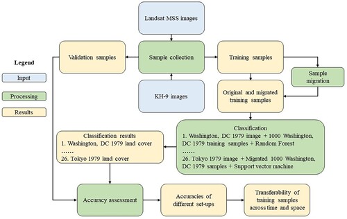
2.2. The experimental design

Two different ways for migrating training samples across time were tested (Table 1). First, all training samples were migrated over time following the approach used by Gong et al. (2019). 1000 training samples were collected from Landsat MSS images of Washington D. C. in 1979 using a KH-9 image acquired in the same year as the reference data. The training samples were used to train models to classify Landsat MSS data in 1979, 1982, and 1984. Second, only unchanged training samples between 1979, 1982, and 1984 were migrated across time following the approach developed by Huang et al. (2020). To reduce errors in migration, we visually judged the changing status of each sample. Two kinds of samples were removed from the sample set, those with changed land cover types and poor quality (e.g. cloud cover) in the later periods. For comparison purposes, a small size of training samples (300) was taken from Landsat MSS data each year and used in classification. The goal is to compare the classification accuracy obtained by migrating a large-size sample set to the accuracy obtained using a current sample set with a size typically used in urban land cover classifications. Urban land cover classification of a single city commonly uses a sample size between 200 and 300 (Li et al. 2014).

Table 1. The setup of the experiment on migrating training samples across time.

Year	Test 1	Test 2	Test 3
1979	1000 samples in 1979	–	300 samples in 1979
1982	1000 samples in 1979	samples unchanged in 1982	300 samples in 1982
1984	1000 samples in 1979	samples unchanged in 1984	300 samples in 1984

Migrating training samples across cities tested the feasibility of conducting region-specific classification. Samples collected from other cities and mixed samples were used in classification (Table 2). Mixed samples correspond to a scenario in that training samples collected in the same urban ecoregion are pooled together to train the classifier. Because Tokyo does not belong to the same ecoregion as Washington, D.C., and Boston, no mixed samples were created for Tokyo. Samples were collected locally and used to classify the Landsat MSS images for comparison purposes. The difference between the classification results based on the migrated and local-specific samples was compared. Furthermore, we migrated the training samples collected in Washington, D. C. to train the classifiers used in Tokyo. We chose 1979 as the baseline time for all cities.

Table 2. The experiment’s setup on migrating training samples across space (WA = Washington, D. C.).

City	Test 4	Test 5	Test 6
WA	1000 WA samples	1000 Boston samples	500 WA + 500 Boston samples
Boston	1000 Boston samples	1000 WA samples	500 WA + 500 Boston samples
Tokyo	1000 Tokyo samples	1000 WA samples	–

2.3. Data collection and pre-processing

Landsat MSS images covering the three cities were extracted from the Landsat MSS archives hosted by the GEE (Table 3). We used the Landsat MSS image available in an entire year, including data collected by MSS sensors onboard landsat2, landsat3, landsat4, and landsat5. The data were resampled into 60 m spatial resolution. All T1-level images and T2-level images whose geometric precision correction residuals are within 30 m were used in the study. KH-9 images for the two cities were downloaded from the USGS’s Earth Resources Observation and Science (EROS) Centre (https://earthexplorer.usgs.gov/). The data has a resolution of 0.6-1.2 m (2–4 feet). KH-9 images were acquired in the tif format, with a size of 9 in.. More details of the used images are listed in Table 3.

Table 3. List of images used in the study (WA = Washington, D. C.).

City	Year	Landsat MSS		KH-9
		Path/row	Number	Image ID
WA	1979	015/033, 016/033, 017/033	72	D3C1215-300737F021
	1982		35	D3C1217-301212F002, D3C1217-301212F003
	1984		44	D3C1219-300947F002
Boston	1979	012/030, 012/031, 013/030, 013/031,014/30	99	D3C1215-200478F003
Tokyo	1979	115/35, 116/35	37	D3C1215-200446F004, D3C1215-200446F005

For Landsat MSS images, automatic cloud and cloud shadow recognition methods were used to mask out pixels contaminated by clouds (Braaten, Cohen, and Yang 2015). The DN values of at 5%, 10%, 50%, 75%, and 95% of bands B1, B2, B3, and B4 of all images were extracted. The maximum values of the Normalized Difference Water Index (NDWI) and the Normalized Difference Vegetation Index (NDVI) were used to improve the water and vegetation signatures, respectively. NASADEM, a Digital Elevation Model (DEM) derived from STRM data, was also included in the study (Crippen et al. 2016). The composite images, therefore, had 23 bands.

A geometric correction was done on KH-9 images before using them as references. The three-order polynomial method, shown to achieve high accuracy in rectifying KH-9 images, was used for geometric correction (Mi et al. 2015). The geometric correction process was run in ArcGIS (version 10.6, ESRI). For each KH-9 image, 30 locations were identified using the high-resolution base map in ArcGIS and used as ground control points (GCPs). Each rectified image was validated using an independent set of ten testing locations. The residual RMSE of all KH-9 images was kept under two pixels (i.e. 2.4 m) with an average RMSE value of 1.63 m.

Training samples were collected from Landsat MSS images using the rectified KH-9 images as references. The sample sizes for each experimental set-up are specified in Table 1 and Table 2. Each sample point contained one pixel. Only pixels that could be visually identified to the class level on both Landsat MSS and KH-9 images were collected. Samples were randomly selected over the entire study area to achieve better representation.

2.4. Classification and validation

The classification system includes six land cover classes: impervious surface, tree cover, grass, water surface, and cropland. Random forest (RF) and Supporting vector machine (SVM) classifiers were used in this study. The purpose was to test whether the two machine learning methods would perform differently with migrated training samples.

For RF, the number of trees was varied between 10 and 500. The split was varied between 2 and 7. For SVM, cost values from 10 to 200 and gamma values from 0.0625 to 2 were tested. The training samples were split by a ratio of 7:3. Only 70% of the samples were used to train the model, and the rest were used as test samples. The classification was cross-validated ten times for each parameter combination, and the mean accuracy was reported as the model accuracy. Models that achieved the highest accuracy were then used to classify the composite images.

The validation samples were collected using an equalized stratified random approach. We randomly assigned 50 samples to each class in the classified result. The samples were then visually interpreted on original images. Based on the interpretation, we built the confusion matrix and estimated the overall accuracy and Kappa coefficient as the indicators of classification accuracy. The entire data collection and classification process is summarized in Figure 1.

Figure 1. Flowchart of the analysis process.

3. Results

3.1. Classification results for migrating training samples across time

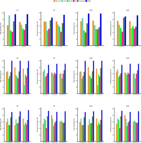
The classification accuracy dropped slightly in 1982 and 1984 based on 1000 samples migrated from 1979 (Table 4). Overall accuracies were reduced by 2% (RF) and 1.33% (SVM) for 1982 and by 3% (RF) and 2.33% (SVM) for 1984. No significant improvements in classification accuracies were obtained by only using unchanged samples from the previous time. For 1979, the overall accuracy based on 1000 samples was2.34% (RF) to3% (SVM) higher than those based on 300 samples. For 1982 and 1984, the classification accuracies obtained using migrated samples were higher or equal to those achieved using 300 samples collected for the current years. The two classifiers achieved similar classification accuracies.

Table 4. Comparison of classification accuracies of different combinations of classifiers and sampling designs in Washington, D. C.

Year	Training samples	Classifier	Overall accuracy	Kappa
1979	1000 samples in 1979	RF	68.67%	0.624
		SVM	68.33%	0.620
	300 samples in 1979	RF	66.33%	0.596
		SVM	65.33%	0.584
1982	1000 samples in 1979	RF	66.67%	0.600
		SVM	67.00%	0.599
	Unchanged samples	RF	67.00%	0.604
		SVM	67.67%	0.612
	300 samples in 1982	RF	65.00%	0.580
		SVM	64.67%	0.576
1984	1000 samples in 1979	RF	65.67%	0.588
		SVM	66.00%	0.592
	Unhanged samples	RF	65.33%	0.584
		SVM	65.00%	0.580
	300 samples in 1984	RF	66.33%	0.595
		SVM	65.33%	0.584

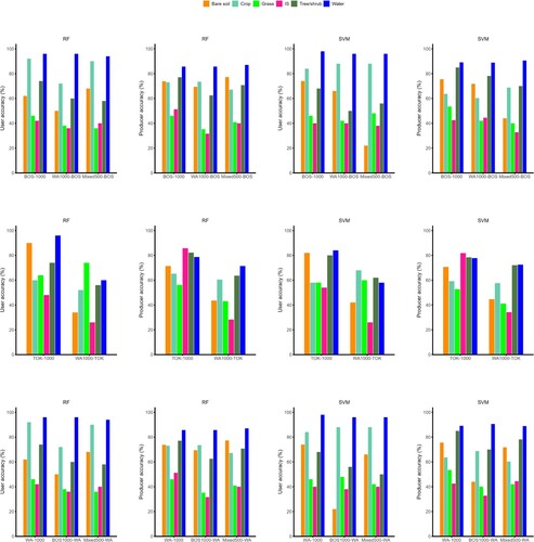
The confusion matrix showed that water was classified most accurately among all land cover classes. The producer and user accuracies of grass and impervious surface class were among the lowest when using migrated training samples (Figure 2).

Figure 2. User and producer accuracies of land cover classification of Washington, D. C. in 1979, 1982, and 1984. RF = Random forest; SVM = Support vector machine; 79-1000 = 1000 samples from 1979 for classifying 1979 images; 79-300 = 300 samples from 1979 for classifying 1979 images; 79-1000-82 = 1000 samples from 1979 used for classifying 1982 images; 79-unc-82 = unchanged samples from 1979 used for classifying 1982 images; 82-300-82 = 300 samples from 1982 used for classifying 1982 images; 79-1000-84 = 1000 samples from 1979 used for classifying 1984 images; 79-unc-84 = unchanged samples from 1979 used for classifying 1984 images; 84-300-84 = 300 samples from 1984 used for classifying 1984 images.

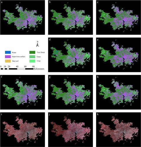
Classification results based on migrated training samples displayed a similar spatial pattern to those based on training samples collected for the current year (Figures 3 and 4).

Figure 3. Classification results of Washington, D. C. using RF classifier. a) 1979 images classified using 1000 samples in 1979; b) 1982 images classified using 1000 samples in 1979; c) 1984 images classified using 1000 samples in 1979; d) 1982 images classified using unchanged samples from 1979; e) 1984 images classified using unchanged samples from 1979; f) 1979 images classified using 300 samples in 1979; g) 1982 images classified using 300 samples in 1982; h) 1984 images classified using 300 samples in 1984; i) the study area in 1979 (Landsat MSS false-color composite image with green, red, and near-infrared bands); j) the study area in 1982; k) the study area in 1984.

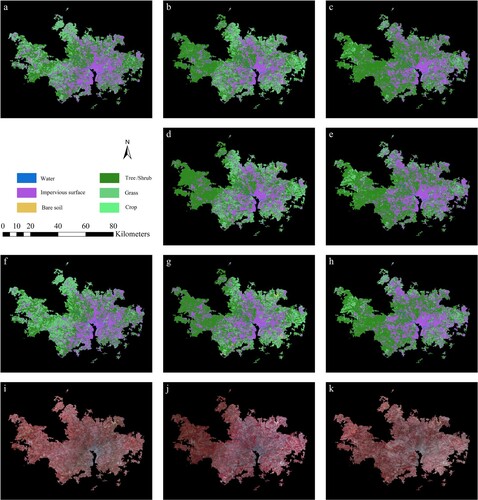
Figure 4. Classification results of Washington, D. C. using SVM classifier. a) 1979 images classified using 1000 samples in 1979; b) 1982 images classified using 1000 samples in 1979; c) 1984 images classified using 1000 samples in 1979; d) 1982 images classified using unchanged samples from 1979; e) 1984 images classified using unchanged samples from 1979; f) 1979 images classified using 300 samples in 1979; g) 1982 images classified using 300 samples in 1982; h) 1984 images classified using 300 samples in 1984; i) the study area in 1979 (Landsat MSS false-color composite image with green, red, and near-infrared bands); j) the study area in 1982; k) the study area in 1984.

3.2. Results for migrating training samples across cities

The classification accuracies of Boston images using the training samples collected in Washington, D. C. were substantially lower than those based on the local samples (Table 5). A 9% and 7% reduction in overall accuracies were observed for RF and SVM classifiers, respectively. The reverse transfer of samples from Boston to be used in Washington, D. C. resulted in a reduction of overall accuracies at the same magnitude (10% and 10.33%). When the mixed samples were used, the loss of overall accuracies was smaller, i.e. 4.34% (Washington, D. C.) and 4% (Boston) when using RF; 4.66% (Washington, D. C.) and 2.67% (Boston) when using SVM.

Table 5. Classification accuracies of the migrating training samples across the space.

City	Training samples	Classifier	Overall accuracy	Kappa
WA	WA 1000 samples	RF	68.67%	0.624
		SVM	68.33%	0.620
	Boston 1000 samples	RF	58.67%	0.504
		SVM	58.00%	0.496
	500 WA + 500 Boston samples	RF	64.33%	0.572
		SVM	63.67%	0.564
Boston	WA 1000 samples	RF	59.33%	0.512
		SVM	60.67%	0.528
	Boston 1000 samples	RF	68.33%	0.619
		SVM	67.67%	0.612
	500 WA + 500 Boston samples	RF	64.33%	0.572
		SVM	65.00%	0.580
Tokyo	WA 1000 samples	RF	50.33%	0.404
		SVM	52.67%	0.432
	Tokyo 1000 samples	RF	72.00%	0.664
		SVM	69.33%	0.632

The reduction of classification accuracy was significant when transferring the samples outside the urban ecoregion. The overall accuracies of land cover classifications of Tokyo using RF and SVM classifiers trained on the migrated samples were 21.67% and 16.66% lower than those trained on the local samples, respectively.

Among the six land cover classes, water had the highest producer and user accuracies for the classification results of Boston based on the migrated samples (Figure 5). In contrast, the impervious surface class had the lowest values. The producer and user accuracies of the impervious surface class improved when RF and the mixed samples were used. The classification results of Washington, D. C. showed the same pattern as Boston’s. The producer and user accuracies of most land cover classes were higher for the classification result of Tokyo based on the local samples than that of classification result based on the migrated samples. Impervious surface class had the lowest accuracy, followed by bare soil for the classifications result of Tokyo based on migrated samples.

Figure 5. User and producer accuracies of land cover classification of Boston, Tokyo, and Washington D. C. in 1979. RF = Random forest; SVM = Support vector machine; Bos-1000 = 1000 samples from Boston for classifying Boston images; WA-1000-Bos = 1000 samples from Washington D. C. for classifying Boston images; Mixed-500-Bos = 500 samples from Washington D. C. and Boston each for classifying Boston images; Tok-1000 = 1000 samples from Tokyo for classifying Tokyo images; WA-1000-Tok = 1000 samples from Washington D. C. for classifying Tokyo images; WA-1000 = 1000 samples from Washington D. C. for classifying Washington D.C. images; Bos-1000-WA = 1000 samples from Boston for classifying Washington D. C. images; Mixed-500-WA = 500 samples from Washington D. C. and Boston each for classifying Washington D. C. images.

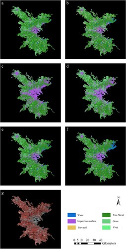
Compared to the classification results using the local samples (Figure 6a and b), impervious surface class in Boston were overclassified in the results based on the migrated samples (Figure 6c and d). The results based on the mixed samples were similar to those using the local samples (Figure 6e and f). The classification results of Washington, D.C. did not show the same pattern as Boston’s (Fig. S1).

Figure 6. Classification results of Boston in 1979. a) RF Classification based on local samples; b) SVM Classification based on local samples; c) RF Classification based on migrated samples; d) SVM Classification based on migrated samples; e) RF Classification based on mixed samples; f) SVM Classification based on mixed samples; g) the study area in 1979 (Landsat MSS false-color composite image with green, red, and near-infrared bands).

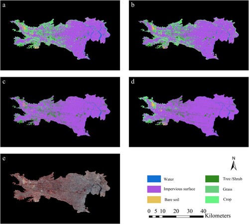
Overestimation of the impervious surface class was also observed in Tokyo. Classification results based on the migrated samples (Figure 7c and d) overestimated the impervious surface class comparing to classification results based on the local samples (Figure 7a and b).

Figure 7. Classification results of Tokyo in 1979. a) RF Classification based on local samples; b) SVM Classification based on local samples; c) RF Classification based on migrated samples; d) SVM Classification based on migrated samples; e) the study area in 1979 (Landsat MSS false-color composite image with green, red, and near-infrared bands).

4. Discussion

4.1. Transferability of training samples across time

Migrating training samples across time resulted in acceptable classification results of urban land cover by using Landsat MSS data. The overall accuracy was only reduced slightly when the migration time was short (∼5 years). These findings corroborate findings from studies conducted using Landsat TM data. Huang et al. (2020) tested the migration of training samples on Landsat TM, ETM+, and Landsat 8 OLI/TIRS. They obtained a classification accuracy of 71.42% in 2010 using migrated samples, close to the classification result in 2015 using the same number of training samples. In another study, samples were migrated from 2020 to 2015 to classify wetlands, and accuracies (>80%) deemed suitable for the study purpose were achieved (Yan and Niu 2021).

The relatively stable classification accuracy obtained using training samples migrated from recent times confirmed the theory of stable classification with limited samples. Gong et al. (2019) showed through an extensive experiment that the mean overall accuracy of the sample reduction is very stable until as few as 40% of the remaining samples are used for global land cover classification. Also, the mean accuracy is within 1% of that obtained with unaltered training samples, even when the error of the training samples reaches 20%. On the global scale, Huang et al. found that 76% of training samples remained unchanged after migrating them from 2015 to 2010. In our study, 925 samples in 1982 and 829 samples in 1984 remained unchanged, even though urban areas are considered places experiencing frequent land cover changes. The number of samples remained unchanged was much higher than the threshold value of 40% cited by Gong et al. (2019) Also, our study results supported their finding that mean accuracy would change within 1% when the error of the training samples reached 20%. When all migrated samples were used in classifications, the changes in accuracy due to the inclusion of samples with wrong labels varied between 0.67% and 1.34% in our study. Furthermore, classification accuracies obtained using all migrated and unchanged samples were higher or equal to those achieved using 300 samples collected specifically for that year. These results indicate that collecting a large size of training samples when good reference data are available and migrating them across time can be a feasible solution for the need for reference data for generating samples from Landsat MSS data.

4.2. Transferability of training samples across space

Migrating samples across cities achieved a different classification accuracy than migrating samples across time in the same city. The reduction of classification accuracy was more significant when migrating the samples to a city not located in the same urban ecoregion. Accuracy reduction can be explained by urban environments’ high heterogeneity and complexity. The representativeness of training samples would decrease outside of the places where they were collected. However, there is regularity in city structure, configuration, constituent elements, and vegetation types within geographic regions and by the level of economic development (Schneider, Friedl, and Potere 2010). The regularity contributes to better accuracy within an urban ecoregion than out of the ecoregion. This is the reason behind the designation of urban ecoregions.

We noted a pattern of over-classification of the impervious surface class using the migrated samples. The pattern may be explained by the coarse resolution of Landsat MSS data and the mislabeled samples in the migrated samples. First, separating impervious surfaces from land cover types such as bare soil and grassland is difficult with medium-resolution satellite data because of the spectral mixture problem (Feng and Fan 2021). Second, migrated training data contain samples with wrong labels due to land cover changes. Mislabeled training samples further reduced the classifier’s ability to differentiate impervious surfaces from other classes. Because more migrated samples were collected from impervious surfaces than from other classes in our study, the classifier trained using the migrated samples would classify more pixels to the impervious surface class.

We found that pooling together training samples from the cities in the same urban ecoregion can achieve better classification results than migrating training samples from one city to another. The finding provided evidence to support the possibility of using urban ecoregions rather than an individual urban area as the unit to collect training samples and run classification. Divide the study area into tiles and collecting training samples to classify each tile is a method used in large-scale land cover classification, e.g. Zhang and Roy (2017) divided the US into 561 tiles with a size of 159 km × 159 km, and Zhang et al. (2021) split the globe into 948 tiles with a size of 5^o × 5^o tiles. However, the method is less frequently used in urban land cover classification. Here we showed that rather than using tiles in regular sizes, using urban ecoregions as the units for classification is also a feasible option.

RF and SVM did not differ significantly in classification accuracies when using the migrated samples. Earlier studies found that RF is relatively insensitive to mislabeled training data (Mellor et al. 2015), while SVM performed well in classifying heterogenous landscapes (Rahman et al. 2020). Our results supported those observations. The two classifiers are suitable for urban land cover classification based on Landsat MSS data.

4.3. Limitation of the current study

While this study proved that the migration of training samples could be a viable solution for collecting training samples to generate urban land cover products using Landsat MSS data, two limitations of the current study must be noted. First, due to the extensive human labor in collecting training and validation samples, we only selected three cities in two urban ecoregions to run the experiment. Conducting tests in more urban ecoregions would help solidify this study’s findings. However, the main result of this study will hold as the underlying theories have already been proven valid by other studies. Second, we only migrated training samples within a short period, i.e. three and five years. Since Landsat MSS data are available from 1972 to 1992, covering the entire period and checking the reduction of classification over time will help identify the limit of migrating training samples.

5. Conclusions

High-quality training samples are essential for classifying satellite data into LULC maps of urban areas. However, obtaining training samples using historical satellite data such as Landsat MSS in large-scale mapping works is a challenging task. Based on the concept of urban ecoregions and the theory of stable classification with limited samples, we came up with a solution, i.e. using KH-9 images as reference data to collect training samples at the regional scale and migrate samples across time and space. Through experiments, we have shown that acceptable classification accuracy could be achieved using this method. While more studies are needed to test the robustness of our proposed solution, findings from this study have great value in tracking the historical urbanization pattern on a global scale with Landsat MSS data.

Acknowledgements

We want to thank the two anonymous reviewers for their constructive comments. Also, we thank graduate students in the laboratory for helping to collect training and validation samples and Google LLC for providing the Google Earth Engine platform.

Disclosure statement

No potential conflict of interest was reported by the author(s).

Data availability statement

Satellite data used in this study can be obtained from https://earthexplorer.usgs.gov/. All training samples and validation samples are included in the supplementary files.

Correction Statement

This article has been corrected with minor changes. These changes do not impact the academic content of the article.

Additional information

Funding

This work was supported by the National Key Research and Development Program of China [grant number 2019YFA0607201].

References

- Braaten, J. D., W. B. Cohen, and Z. Yang. 2015. “Automated Cloud and Cloud Shadow Identification in Landsat MSS Imagery for Temperate Ecosystems.” Remote Sensing of Environment 169: 128–138. doi:10.1016/j.rse.2015.08.006.
- Chen, M., H. Zhang, W. Liu, and W. Zhang. 2014. “The Global Pattern of Urbanization and Economic Growth: Evidence from the Last Three Decades.” PLoS ONE 9 (8): e103799. doi:10.1371/journal.pone.0103799.
- Congalton, R. G., R. G. Oderwald, and R. A. Mead. 1983. “Assessing Landsat Classification Accuracy Using Discrete Multivariate Analysis Statistical Techniques.” Photogrammetric Engineering & Remote Sensing 49 (12): 1671–1678.
- Crippen, R., S. Buckley, P. Agram, E. Belz, E. Gurrola, S. Hensley, M. Kobrick, et al. 2016. “Nasadem Global Elevation Model: Methods and Progress.” The International Archives of the Photogrammetry, Remote Sensing and Spatial Information Sciences XLI-B4: 125–128. doi:10.5194/isprs-archives-XLI-B4-125-2016.
- Feng, S., and F. Fan. 2021. “Impervious Surface Extraction Based on Different Methods from Multiple Spatial Resolution Images: A Comprehensive Comparison.” International Journal of Digital Earth 14 (9): 1148–1174. doi:10.1080/17538947.2021.1936227.
- Friedl, M. A., D. Sulla-Menashe, B. Tan, A. Schneider, N. Ramankutty, A. Sibley, and X. Huang. 2010. “MODIS Collection 5 Global Land Cover: Algorithm Refinements and Characterization of new Datasets.” Remote Sensing of Environment 114 (1): 168–182. doi:10.1016/j.rse.2009.08.016.
- Ghorbanian, A., M. Kakooei, M. Amani, S. Mahdavi, A. Mohammadzadeh, and M. Hasanlou. 2020. “Improved Land Cover map of Iran Using Sentinel Imagery Within Google Earth Engine and a Novel Automatic Workflow for Land Cover Classification Using Migrated Training Samples.” ISPRS Journal of Photogrammetry and Remote Sensing 167: 276–288. doi:10.1016/j.isprsjprs.2020.07.013.
- Gong, P., X. Li, J. Wang, Y. Bai, B. Chen, T. Hu, X. Liu, et al. 2020. “Annual Maps of Global Artificial Impervious Area (GAIA) Between 1985 and 2018.” Remote Sensing of Environment 236: 111510. doi:10.1016/j.rse.2019.111510.
- Gong, P., H. Liu, M. Zhang, C. Li, J. Wang, H. Huang, N. Clinton, et al. 2019. “Stable Classification with Limited Sample: Transferring a 30-m Resolution Sample set Collected in 2015 to Mapping 10-m Resolution Global Land Cover in 2017.” Science Bulletin 64 (6): 370–373. doi:10.1016/j.scib.2019.03.002.
- Gurney, C. M. 1981. “The use of Contextual Information to Improve Land Cover Classification of Digital Remotely Sensed Data.” International Journal of Remote Sensing 2 (4): 379–388. doi:10.1080/01431168108948372.
- Herold, M., N. C. Goldstein, and K. C. Clarke. 2003. “The Spatiotemporal Form of Urban Growth: Measurement, Analysis and Modeling.” Remote Sensing of Environment 86 (3): 286–302. doi:10.1016/S0034-4257(03)00075-0.
- Huang, H., J. Wang, C. Liu, L. Liang, C. Li, and P. Gong. 2020. “The Migration of Training Samples Towards Dynamic Global Land Cover Mapping.” ISPRS Journal of Photogrammetry and Remote Sensing 161: 27–36. doi:10.1016/j.isprsjprs.2020.01.010.
- Huang, C., J. Yang, N. Clinton, L. Yu, H. Huang, I. Dronova, and J. Jin. 2021. “Mapping the Maximum Extents of Urban Green Spaces in 1039 Cities Using Dense Satellite Images.” Environmental Research Letters 16 (6): 064072. doi:10.1088/1748-9326/ac03dc.
- Karra, K., C. Kontgis, Z. Statman-Weil, J. C. Mazzariello, M. M. Mathis, and S. P. Brumby. 2021. “Global land use / land cover with Sentinel 2 and deep learning.” 2021 IEEE International Geoscience and Remote Sensing Symposium IGARSS, Brussels, Belgium, 2021, pp. 4704–4707. doi:10.1109/IGARSS47720.2021.955349.
- Li, C., J. Wang, L. Wang, L. Hu, and P. Gong. 2014. “Comparison of Classification Algorithms and Training Sample Sizes in Urban Land Classification with Landsat Thematic Mapper Imagery.” Remote Sensing 6 (2): 964–983. doi:10.3390/rs6020964.
- Liu, H., P. Gong, J. Wang, N. Clinton, Y. Bai, and S. Liang. 2020. “Annual Dynamics of Global Land Cover and its Long-Term Changes from 1982 to 2015.” Earth System Science Data 12 (2): 1217–1243. doi:10.5194/essd-12-1217-2020.
- Liu, X., G. Hu, Y. Chen, X. Li, X. Xu, S. Li, F. Pei, and S. Wang. 2018. “High-resolution Multi-Temporal Mapping of Global Urban Land Using Landsat Images Based on the Google Earth Engine Platform.” Remote Sensing of Environment 209: 227–239. doi:10.1016/j.rse.2018.02.055.
- Melchiorri, M., A. J. Florczyk, S. Freire, M. Schiavina, M. Pesaresi, and T. Kemper. 2018. “Unveiling 25 Years of Planetary Urbanization with Remote Sensing: Perspectives from the Global Human Settlement Layer.” Remote Sensing 10 (5): 768. doi:10.3390/rs10050768.
- Mellor, A., S. Boukir, A. Haywood, and S. Jones. 2015. “Exploring Issues of Training Data Imbalance and Mislabelling on Random Forest Performance for Large Area Land Cover Classification Using the Ensemble Margin.” ISPRS Journal of Photogrammetry and Remote Sensing 105: 155–168. doi:10.1016/j.isprsjprs.2015.03.014.
- Mi, H., G. Qiao, T. Li, and S. Qiao. 2015. “Declassified Historical Satellite Imagery from 1960s and Geometric Positioning Evaluation in Shanghai, China.” In Geo-Informatics in Resource Management and Sustainable Ecosystem. GRMSE 2014. Communications in Computer and Information Science, Vol 482, edited by F. Bian, and Y. Xie, 283–292. Berlin, Germany: Springer, Berlin, Heidelberg.
- Naboureh, A., A. Li, H. Ebrahimy, J. Bian, M. Azadbakht, M. Amani, G. Lei, and X. Nan. 2021. “Assessing the Effects of Irrigated Agricultural Expansions on Lake Urmia Using Multi-Decadal Landsat Imagery and a Sample Migration Technique Within Google Earth Engine.” International Journal of Applied Earth Observation and Geoinformation 105: 102607. doi:10.1016/j.jag.2021.102607.
- Nowosad, J., T. F. Stepinski, and P. Netzel. 2019. “Global Assessment and Mapping of Changes in Mesoscale Landscapes: 1992–2015.” International Journal of Applied Earth Observation and Geoinformation 78: 332–340. doi:10.1016/j.jag.2018.09.013.
- Pesaresi, M., and P. Politis. 2022. “GHS Built-up Surface Grid, Derived from Sentinel2 Composite and Landsat, Multitemporal (1975-2030).” European Commission, Joint Research Centre. Accessed July 20, 2023. doi:10.2905/9F06F36F-4B11-47EC-ABB0-4F8B7B1D72EA
- Phan, D. C., T. H. Trung, V. T. Truong, T. Sasagawa, T. P. T. Vu, D. T. Bui, M. Hayashi, T. Tadono, and K. N. Nasahara. 2021. “First Comprehensive Quantification of Annual Land use/Cover from 1990 to 2020 Across Mainland Vietnam.” Scientific Reports 11 (1): 9979. doi:10.1038/s41598-021-89034-5.
- Qiu, C., M. Schmitt, C. Geiß, T. K. Chen, and X. X. Zhu. 2020. “A Framework for Large-Scale Mapping of Human Settlement Extent from Sentinel-2 Images via Fully Convolutional Neural Networks.” ISPRS Journal of Photogrammetry and Remote Sensing 163: 152–170. doi:10.1016/j.isprsjprs.2020.01.028.
- Rahman, A., H. M. Abdullah, M. T. Tanzir, M. J. Hossain, B. M. Khan, M. G. Miah, and I. Islam. 2020. “Performance of Different Machine Learning Algorithms on Satellite Image Classification in Rural and Urban Setup.” Remote Sensing Applications: Society and Environment 20: 100410. doi:10.1016/j.rsase.2020.100410.
- Saleem, A., R. Corner, and J. Awange. 2018. “On the Possibility of Using CORONA and Landsat Data for Evaluating and Mapping Long-Term LULC: Case Study of Iraqi Kurdistan.” Applied Geography 90: 145–154. doi:10.1016/j.apgeog.2017.12.007.
- Schneider, A., M. A. Friedl, and D. Potere. 2010. “Mapping Global Urban Areas Using MODIS 500-m Data: New Methods and Datasets Based on ‘Urban Ecoregions’.” Remote Sensing of Environment 114 (8): 1733–1746. doi:10.1016/j.rse.2010.03.003.
- Seto, K. C., and M. Fragkias. 2005. “Quantifying Spatiotemporal Patterns of Urban Land-use Change in Four Cities of China with Time Series Landscape Metrics.” Landscape Ecology 20 (7): 871–888. doi:10.1007/s10980-005-5238-8.
- Toll, D. L. 1985a. “Analysis of Digital LANDSAT MSS and SEASAT SAR Data for use in Discriminating Land Cover at the Urban Fringe of Denver, Colorado.” International Journal of Remote Sensing 6 (7): 1209–1229. doi:10.1080/01431168508948273.
- Toll, D. L. 1985b. “Landsat-4 Thematic Mapper scene characteristics of a suburban and rural area (USA).” Palaeogeography, Palaeoclimatology, Palaeoecology 49 (9): 355–382. doi:10.1016/0031-0182(85)90061-6.
- Wang, M., D. Mao, Y. Wang, K. Song, H. Yan, M. Jia, and Z. Wang. 2022. “Annual Wetland Mapping in Metropolis by Temporal Sample Migration and Random Forest Classification with Time Series Landsat Data and Google Earth Engine.” Remote Sensing 14 (13): 3191. doi:10.3390/rs14133191.
- Witt, R. G., T. B. Minor, and R. S. Sekhon. 2007. “Use of HCMM Thermal Data to Improve Accuracy of MSS Land-Surface Classification Mapping.” International Journal of Remote Sensing 6 (10): 1623–1636. doi:10.1080/01431168508948310.
- Yan, X., and Z. Niu. 2021. “Reliability Evaluation and Migration of Wetland Samples.” IEEE Journal of Selected Topics in Applied Earth Observations and Remote Sensing 14: 8089–8099. doi:10.1109/JSTARS.2021.3102866.
- Zhang, X., L. Liu, X. Chen, Y. Gao, S. Xie, and J. Mi. 2021. “GLC_FCS30: Global Land-Cover Product with Fine Classification System at 30 m Using Time-Series Landsat Imagery.” Earth System Science Data 13 (6): 2753–2776. doi:10.5194/essd-13-2753-2021.
- Zhang, H. K., and D. P. Roy. 2017. “Using the 500 m MODIS Land Cover Product to Derive a Consistent Continental Scale 30 m Landsat Land Cover Classification.” Remote Sensing of Environment 197: 15–34. doi:10.1016/j.rse.2017.05.024.
- Zhu, Q., Y. Wang, J. Liu, X. Li, H. Pan, and M. Jia. 2021. “Tracking Historical Wetland Changes in the China Side of the Amur River Basin Based on Landsat Imagery and Training Samples Migration.” Remote Sensing 13 (11): 2161. doi:10.3390/rs13112161.