A new multi-source remote sensing image sample dataset with high resolution for flood area extraction: GF-FloodNet

ABSTRACT

Deep learning algorithms show good prospects for remote sensing flood monitoring. They mostly rely on huge amounts of labeled data. However, there is a lack of available labeled data in actual needs. In this paper, we propose a high-resolution multi-source remote sensing dataset for flood area extraction: GF-FloodNet. GF-FloodNet contains 13388 samples from Gaofen-3 (GF-3) and Gaofen-2 (GF-2) images. We use a multi-level sample selection and interactive annotation strategy based on active learning to construct it. Compare with other flood-related datasets, GF-FloodNet not only has a spatial resolution of up to 1.5 m and provides pixel-level labels, but also consists of multi-source remote sensing data. We thoroughly validate and evaluate the dataset using several deep learning models, including quantitative analysis, qualitative analysis, and validation on large-scale remote sensing data in real scenes. Experimental results reveal that GF-FloodNet has significant advantages by multi-source data. It can support different deep learning models for training to extract flood areas. There should be a potential optimal boundary for model training in any deep learning dataset. The boundary seems close to 4824 samples in GF-FloodNet. We provide GF-FloodNet at https://www.kaggle.com/datasets/pengliuair/gf-floodnet and https://pan.baidu.com/s/1vdUCGNAfFwG5UjZ9RLLFMQ?pwd=8v6o.

KEYWORDS:

• Flood area extraction
• dataset construction
• multi-source remote sensing data
• deep learning

View correction statement:

Correction

1. Introduction

In recent years, flood disasters have occurred frequently around the world, causing great damage (Wang and Ding 2022; Rentschler, Salhab, and Jafino 2022). Satellite remote sensing technology is widely used in flood monitoring, because it can effectively and accurately observe the occurrence of flood events, facilitate rapid response to floods, and reduce unnecessary damage (Tralli et al. 2005).

Both multispectral (MS) remote sensing and synthetic aperture radar (SAR) remote sensing can be used for flood monitoring. MS images have rich spectral information and high image resolution, which are suitable for dynamic monitoring and analysis of many surface processes, especially Landsat-7/8, Sentinel-2, Planet, GF-1/2, and other optical satellites provide us with more reliable and detailed images. However, optical sensors are susceptible to the influence of cloud cover. During floods due to heavy or persistent rainfall, cloud cover is often high, making it is difficult for flood monitoring using MS remote sensing images (Jiang et al. 2021). SAR is an active microwave remote sensing technology with the advantage of all-weather, all-day operation. It is able to penetrate clouds for detection in cloudy and rainy weather and thus has great potential for application in the field of flood monitoring (Singha et al. 2020). Nevertheless, there are some difficulties in using SAR images to extract flood areas. For example, the shadow of mountains may interfere with the detection of flood areas. Wind or heavy rainfall may cause water surface roughness and affect the extraction of flood areas in SAR images. Therefore, the combination of MS remote sensing images and SAR remote sensing images can achieve the complementary advantages of each, which is more beneficial to improve the effectiveness of remote sensing flood monitoring.

Most application studies in remote sensing flood monitoring are carried out based on SAR images. The mainstream methods of them include histogram thresholding (Tiwari et al. 2020; Liang and Liu 2020) or clustering (Martinis, Plank, and Ćwik 2018; Martinis, Twele, and Voigt 2009), fuzzy classification (Martinis, Kersten, and Twele 2015; Twele et al. 2016), region growing (Mason et al. 2012; Ouled Sghaier et al. 2018), texture analysis (Pradhan et al. 2014; Senthilnath et al. 2013; Amitrano et al. 2018) and machine learning (Benoudjit and Guida 2019; Tavus, Kocaman, and Gokceoglu 2022). There are fewer studies that use only MS images for flood monitoring. The studies are mainly developed based on the Normalized Difference Water Index (NDWI) and traditional machine learning (Wang, Zhang, and Leung 2019; Son, Chen, and Chen 2021; Kool et al. 2022). Because of the complementary nature of SAR and MS data, some studies combine them for flood monitoring and achieve good results, but most of them blend SAR data with NDWI (Vanama, Rao, and Bhatt 2021; Anusha and Bharathi 2020; Tavus et al. 2020; Benoudjit and Guida 2019; Manakos, Kordelas, and Marini 2020; Slagter et al. 2020; Goffi et al. 2020; Tavus, Kocaman, and Gokceoglu 2022).

These traditional methods mentioned above are simple to implement but perform poorly in capturing complex features related to floods. By contrast, deep learning methods can consider both pixel intensity and spatial correlation of neighbouring pixels, and outperform traditional methods due to their more powerful feature learning capabilities. Recently, there are a large number of deep learning methods introduced into the remote sensing information extraction process and play an important role in the field of flood monitoring (Nemni et al. 2020; Mateo-Garcia et al. 2021; Rambour et al. 2020; Bonafilia et al. 2020; Zhao, Sui, and Liu 2023; Li and Demir 2023; Wang et al. 2022; Hamidi et al. 2023; Bai et al. 2021; Drakonakis et al. 2022; Konapala, Kumar, and Ahmad 2021; He et al. 2023). Most deep learning methods rely on the large amounts of labeled training samples to optimize model parameters. However, there is a lack of labeled image datasets in the field of flood monitoring. Because there are few high-resolution images available for floods with suddenness and short duration. In addition, the annotation cost of remote sensing images is very high.

As listed in Table 1, some public flood-related image datasets have been proposed. Rahnemoonfar et al. (2021) provide a high-resolution (1.5 cm) Unmanned Aerial Vehicle (UAV) image dataset with pixel-level annotations named FloodNet. Based on FloodNet, the authors compare several methods’ performance, including classification, semantic segmentation, and visual question answering (VQA). But this paper doesn’t introduce data from other sources to implement multi-source segmentation. Despite the very high spatial resolution of UAV images, UAV observations don’t have as wide coverage as satellite observations. In practice, it is difficult to extract large-scale flood areas using only UAV images. Bonafilia et al. (2020) propose Sen1floods11 dataset for training and validation of deep learning methods for flood detection on Sentinel-1 remote sensing images. The dataset contains 4831 chips of 512 × 512 10 m pixels, among which, 4370 chips are automatically labeled using thresholding methods, only 446 chips are hand labeled. Although the paper provides Sentinel-1/2 multi-source labeled samples, Sentinel-1 and Sentinel-2 are used separately for experimental comparison. The two types of samples don’t share the same labels, and are not combined for multi-source flood detection. Rambour et al. (2020) utilize both Sentinel-1 and Sentinel-2 images to construct a new SEN12-FLOOD Dataset for flood detection. They use several deep networks for multi-source time series analysis to classify the images in the dataset. However, this dataset only provides image-level labels for scene classification, rather than pixel-level labels for flood segmentation. Similarly, Sentinel Flooding Sequences Dataset (Bischke et al. 2019) consists of 10 m Sentinel-2 images without pixel-level labels. WorldFloods (Mateo-Garcia et al. 2021) provides pixel-level labeled Sentinel-2 samples for flood area extraction, not involved other data sources. The Global Flood Database (Tellman et al. 2021) includes multi-source remote sensing data including Landsat, MODIS data, etc., but its pixel-level labels are generated from thresholding methods. The authors don’t carry out multi-source flood monitoring on it.

Table 1. Part of the public flood-related image datasets.

Dataset	Data Source	Satellite Imagery	Highest Spatial Resolution	Pixel-Level Labels	Multi-Source Dataset	Using Multi-Source Data for Flood Monitoring
FloodNet (Rahnemoonfar et al. 2021)	Unmanned Aerial Vehicle	No	1.5cm	✓	✗	✗
Sentinel Flooding Sequences Dataset (Bischke et al. 2019)	Sentinel-2	Yes	10m	✗	✗	✗
WorldFloods (Mateo-Garcia et al. 2021)	Sentinel-2	Yes	10m	✓	✗	✗
Sen1floods11 (Bonafilia et al. 2020)	Sentinel 1-2	Yes	10m	✓	✓	✗
SEN12-FLOOD (Rambour et al. 2020)	Sentinel 1-2	Yes	10m	✗	✓	✓
The Global Flood Database (Tellman et al. 2021)	Landsat, MODIS, etc.	Yes	250m	✓	✓	✗

These datasets cannot simultaneously meet the requirements of high spatial resolution, with pixel-level labels, and making full use of multi-source data for flood monitoring. In addition, the construction of these datasets either relies on traditional manual annotation or automatic annotation by thresholding methods, so the efficiency and quality are difficult to guarantee at the same time. Also, the construction has not yet considered who are important samples in the dataset. Therefore, it is very necessary to construct a high-quality multi-source remote sensing image dataset with higher resolution for flood area extraction. It is conducive to promoting the application and development of artificial intelligence methods, such as deep learning, in the field of flood monitoring.

We construct the GF-FloodNet dataset using GF-3 SAR images and GF-2 MS images, providing pixel-level labels of flood areas. We will make our dataset publicly available online soon. The dataset construction innovatively uses a multi-level sample selection and interactive annotation process based on active learning. This process is beneficial to the common deep learning models to achieve better performances with fewer labeled samples and significantly reduces the cost of manual annotation. We comprehensively validate and evaluate the GF-FloodNet dataset using several deep learning methods, which fully proves that our dataset can provide good training samples for flood area extraction.

The paper is organized as follows. Section 2 presents the details of the dataset. Section 3 presents the experimental results. Sections 4 and 5 present the discussion and conclusions, respectively.

2. The GF-FloodNet dataset

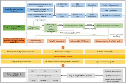
In this section, we introduce the GF-FloodNet dataset in detail, including data sources, dataset construction process, dataset organization, dataset characteristics and application value, dataset validation and evaluation (this part is described in Section 3). The overall framework is shown in Figure 1.

Figure 1. The overall framework of the GF-FloodNet dataset construction.

2.1. Overview of data sources

We use GF-3 SAR images and GF-2 MS images to construct the dataset. The images are collected from seven countries around the world, including Australia, Brazil, China, India, Pakistan, Russia, and South Africa, covering eight flood events. The basic information statistics of the original remote sensing data are shown in Table 2. All the GF-2 MS images contain four bands of Blue, Green, Red and NIR (Near Infrared). As listed in Table 2, the imaging mode of the GF-3 SAR images includes UFS (Ultra-Fine Stripmap), FSI (Fine Stripmap 1) and FSII (Fine Stripmap 2). The corresponding polarization mode includes HH (Horizontal polarization for transmit and Horizontal polarization receive), HV (Horizontal polarization for transmit and Vertical polarization receive).

Table 2. The basic information statistics of the original remote sensing data.

Sampling Region	Data Source	GF-3 Imaging Mode& Polarization Mode	Date	Spatial Resolution
Australia	GF-3 L2	UFS & HH	20220301	1.5m
	GF-2 L1A		20220228	4m
Brazil	GF-3 L2	UFS & HH	20220224	1.5m
	GF-2 L1A		20220223	4m
China	GF-3 L2	FSII & HV	20211010	5m
	GF-2 L1A		20211018	4m
India	GF-3 L2	FSI & HV	20220808	2.5m
	GF-2 L1A		20220822	4m
Pakistan	GF-3 L2	FSII & HV	20220902	5m
	GF-2 L1A		20220828	4m
Russia	GF-3 L2	FSII & HV	20220502	5m
	GF-2 L1A		20220503	4m
Russia Presoy	GF-3 L2	FSII & HV	20220502	5m
	GF-2 L1A		20220419	4m
South Africa	GF-3 L2	UFS & HH	20220421	1.5m
	GF-2 L1A		20220402	4m

2.2. Dataset construction

In natural conditions, the distribution of flood areas is usually uneven and not concentrated. Flood areas with different characteristics often exist in complex scenarios. This poses a challenge to sample selection and annotation in the process of dataset construction. Therefore, we use a multi-level sample selection and interactive annotation strategy based on active learning to select and annotate samples. The specific process for dataset construction is as follows.

2.2.1. Collection of data involving flood events from large databases and data preprocessing

The original images consist of the remote sensing data from the Gaofen series satellites, which include both MS and SAR images. To determine the geographic and temporal coverage, we first conduct preliminary searches of flood events on open data websites such as the Global Flood Database (Tellman et al. 2021), Global Disaster Data Platform (https://www.gddat.cn/), and FloodList (https://floodlist.com/). Then, we perform a large-scale data retrieval to screen the eligible GF-3 L2 data on the data center of the China Remote Sensing Satellite Ground Station (CRSSGS). Based on this retrieval, the geographic scope is further narrowed to screen the GF-2 L1A data (cloud coverage is less than 10%) from the same region about one month before and after. During the above retrieval, it is required to visually interpret whether there are flood areas to be labeled. We repeat the above process until we have enough scenes of data.

We preprocess the original SAR and MS images separately using ENVI 5.3 software (available online at https://envi.geoscene.cn/), including filter processing, RPC orthorectification, image registration, resampling, band combination, etc. Firstly, we apply the Enhanced Lee Filter to GF-3 L2 data to effectively suppress the speckle noise caused by the coherence principle of SAR imaging system. Then, the GF-2 L1A MS data are corrected by RPC orthorectification to eliminate the geometric distortion caused by the terrain fluctuation and other factors. According to the corrected projection coordinate system, the corresponding GF-3 L2 data of the same region are projected to make them in the same projection coordinate system. Next, the GF-3 and GF-2 images covering the same region are registered with the GF-2 image as the reference. Through the automatic image registration tool of ENVI 5.3, the maximum number of ground control points and the minimum error value are set. The automatically selected control points are further filtered to reduce the error and complete the image registration operation. After registration, we take the higher resolution image as the reference and resample the other one to the same resolution with cubic convolution interpolation. In this way, we obtain multi-source remote sensing images with the same resolution, crop their overlap regions and perform layer stacking on them. The multi-source data are arranged according to the original band order of the MS images and the single SAR image. Each channel of the combined images covers the same area and is sampled to the same resolution. We store the images in TIFF format and crop them into 13388 patches (256 × 256 pixels) with no overlapping areas.

2.2.2. Sample selection strategy for medium regions

The pixel-level annotation process of remote sensing images is very cumbersome, and the annotation cost is generally higher than that of natural images. Considering that when new flood events occur, we may need to annotate local real-time data for emergency relief. How to construct a labeled dataset efficiently with less cost has more practical implications.

As far as we know, for the difficulty of labeling samples in deep learning, especially in computer vision, active learning (Liu et al. 2022) has been adopted in many studies to alleviate it and enable the model to achieve better performance with fewer labeled samples. It is mainly applied to image classification tasks (Tuia et al. 2011; Yuan et al. 2019; Liu, Zhang, and Eom 2016; Joshi, Porikli, and Papanikolopoulos 2009; Ruiz et al. 2014; Matiz and Barner 2019; Beluch et al. 2018; Lei et al. 2021), although there are also applications to semantic segmentation tasks (Sourati et al. 2019; Yang et al. 2017; Ozdemir et al. 2021; Mahapatra et al. 2018; Rangnekar, Kanan, and Hoffman 2023; Saidu and Csató 2021; Mackowiak et al. 2018; Belharbi et al. 2021; Sinha, Ebrahimi, and Darrell 2019; Gorriz et al. 2017), most of which are based on medical images or natural images. In contrast, it is not widely used in the field of remote sensing semantic segmentation (Lenczner et al. 2022; Desai and Ghose 2022). And the starting point of most related studies is simply to optimize the training process to improve the model performance from the perspective of algorithm research.

Unlike the algorithm research, this paper cuts from the perspective of the dataset and uses a sample selection strategy based on active learning for medium regions. The meaning of ‘medium regions’ refers to 256 × 256 pixels sample patches that require annotation. We rationally select the sample query strategy to achieve accurate recommendations of flood event labeling regions, so that we realize the dual purpose of efficiently constructing high-quality datasets and minimizing the manual annotation cost. The specific procedure is shown in Figure 2.

Figure 2. Illustration of the sample selection strategy based on active learning.

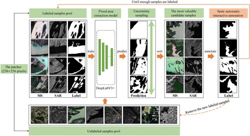
We use DeepLabV3 + as the flood area extraction model because of its excellent performance, which has been demonstrated in existing studies. In fact, other typical models that perform well in flood area extraction tasks can also be used. The number of initial samples about starting active learning varies from case to case. The initial samples need to support the initial training of the flood area extraction model while leaving a lot of room for improvement. But the initial samples should not be too many, otherwise it will lose the significance of reducing the annotation cost.

Therefore, for the patches from the data collection in Section 2.2.1, in the initial stage, we annotate a small number of them (200 patches) for training the flood area extraction model. The number of initial samples is chosen empirically, and subsequent experiments also prove that this initial number is appropriate. These samples correspond to the labeled samples pool in Figure 2. The other patches constitute the unlabeled samples pool, and the model predicts the unlabeled samples in the pool. According to the prediction results, the most valuable candidate samples are selected using an uncertainty sampling query strategy for semi-automatic interactive annotation (as described in Section 2.2.3). Finally, these samples are added to the labeled samples pool, and the model is iteratively trained. We repeat the above process until enough samples are labeled.

In the above process, uncertainty sampling is one of the most commonly used query strategies in active learning, which can be used to measure the value of the samples to the flood area extraction model. The most uncertain samples are also the most valuable to the model because they contain the most information. The model can learn more from these least distinguishable samples. We adopt least confidence as our uncertainty sampling strategy in this paper. The details are given in Equations (1) - (2). We calculate the least confidence of the prediction results of candidate samples as their uncertainty scores. The candidate samples are sorted in descending order based on their respective uncertainty scores. Samples with higher uncertainty are perceived to be more valuable because they are likely to contain more information. Thus, they are preferentially labeled and used to train the model. (1) $LC\left(x\right)=1-P_{\theta }\left({\hat{y}}_{\theta }\right|x\left)\right)$(1) (2) $LC\left(S\right)=\sum _{x\in S}LC\left(x\right)$(2) where $x$ represents a pixel of a sample, $S$ represents a sample, $\theta$ represents the model parameters, and ${\hat{y}}_{\theta }$ is the model's predicted label for $x$. $P_{\theta }\left({\hat{y}}_{\theta }\right|x)$ represents the prediction probability of ${\hat{y}}_{\theta }$ by the model. $LC\left(x\right)$ represents the least confidence of the pixel $x$, $LC\left(S\right)$ represents the least confidence of the sample $S$. When $LC\left(S\right)$ is larger, the model is less confident about the sample $S$, indicating the sample is of greater uncertainty and thus more valuable for the model.

2.2.3. Semi-automatic interactive annotation for specific small flood areas

Following the previous step, in combination with the information extraction module of the PIE-Basic 6.3 software (available online at https://www.piesat.cn/), we perform semi-automatic interactive annotation of the selected candidate samples. The annotation process is illustrated in Figure 3.

Figure 3. Illustration of semi-automatic interactive annotation process.

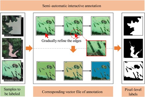
We use the ‘magic wand’ tool of the PIE-Basic 6.3 to semi-automatically annotate the samples. First, combined with visual interpretation, we click on the flood areas in the sample image. The software calculates the difference between the RGB mean value of the selected center point and the surrounding pixels by the seed region growing algorithm. The pixels whose difference value conforms to the preset threshold are selected to be labeled and extracted. These extracted pixels are connected to form the current flood area label, which realizes a semi-automatic interactive annotation. As shown in the second column of the first row of Figure 3, the solid green line outlines the boundary of the current label. For the sake of understanding, the second column of the third row shows the vector file corresponding to the current label, and the labeled area is filled in green to make it easier to see. Then, the above steps are repeated, and the unlabeled flood area is clicked several times. The adjacent areas are merged and the edges are gradually refined. Columns 2 to 4 of Figure 3 show this step-by-step process.

During the annotation process, incorrect parts can be corrected manually to achieve quality control at any time. This can be achieved using the ‘element shaping’ and ‘element cropping’ tools provided by PIE-Basic 6.3. For example, if the boundary of some flood areas spills into the adjacent bare soil, we can add or delete the vertices on the boundary and adjust their positions, so as to correct the labeled area. Alternatively, we can crop the labeled area to remove the overflow parts and then adjust the edge of the cropped area.

After the annotation is completed, we generate the annotation vector file by the ‘vector generation’ tool and then rasterize the vector file by ArcGIS10.2 software (available online at https://www.esri.com/). All labels are stored in TIFF format. Finally, we get the pixel-level labels with a pixel value of 1 for the flood area and 255 for the non-flood area.

It can be seen that our semi-automatic interactive annotation realizes the quality control through manual correction, and completes the annotation faster and more accurately, which can help us obtain the similar or even higher quality labels than manual annotation. Its essence is still manual annotation, but the annotation effect is improved by means of semi-automatic interaction. As shown in the fifth column of the Figure 3, the boundaries are very accurate and detailed, while it is difficult to achieve the same effect by manual annotation only. Therefore, our high-quality labels enable the trained model to perform well, not worse than manual labels.

2.3. Dataset organization

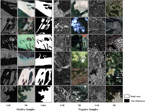
Through the above dataset construction process, we obtain the multi-source remote sensing image sample dataset for flood area extraction: GF-FloodNet. It consists of 13388 image samples and their corresponding pixel-level labels, stored in TIFF format. The spatial resolutions include 1.5, 2.5, and 4 m. Each sample patch is 256 × 256 pixels (384m × 384 m, 640m × 640 m, 1024m × 1024 m). Among them, 4178 samples contain flood areas and 9210 samples do not contain flood areas at all. The statistics on the number of samples in each region are shown in Figure 4. An example of positive and negative samples is shown in Figure 5.

Figure 4. Statistics on the number of samples in each region.

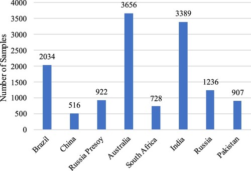
Figure 5. An example of positive and negative samples. The left three columns show some positive samples (containing flood areas), which respectively represent SAR data, MS data, and labels covering the same region. The right four columns show some of the negative samples (containing only non-flood areas) representing SAR and MS covering the same region. The white pixels in the label represent flood areas and the black ones represent non-flood areas.

2.4. Dataset characteristics and application value

High-quality remote sensing satellite image datasets are extremely important for flood monitoring. In this paper, we collect the remote sensing data of GF-3 and GF-2 and construct the target dataset by a multi-level sample selection and interactive annotation strategy based on active learning. The GF-FloodNet dataset has the following characteristics.

1. Sampling from multiple regions worldwide: This dataset is of a certain size, including 13388 remote sensing image samples collected from 7 countries in the global scope.

2. Multi-source advantages: The dataset proposed in this paper contains MS-SAR multi-source image samples covering the same area, which has significant advantages on flood area extraction. We will discuss the multi-source advantages in detail in Section 4.1.Users can choose to use single-source images or multi-source images according to their actual needs.

3. Rich intra-class diversity: The flood areas in this dataset include a variety of common types such as lakes, rivers, and paddy fields with different morphological characteristics, and the non-flood areas include various background object types such as mountains, buildings, cultivated land, vegetation, roads, etc.

4. Multiple high spatial resolutions: The spatial resolutions of remote sensing images in this dataset include 1.5, 2.5, and 4 m, which is conducive to improving the extraction effect and generalization ability of the model.

5. All samples and labels contain geographic information: Unlike other image datasets composed of samples in JPG or PNG format, the samples in our dataset are stored in TIFF format. Each sample and label has geographic coordinates corresponding to the location in the original remote sensing data.

6. Open source and non-profit: The dataset proposed in this paper is publicly and freely available for non-profit related scientific research.

The pixel-level annotated images of the GF-FloodNet dataset can provide training samples for flood area extraction based on deep learning. The models trained on this dataset can be used for practical applications of intelligent remote sensing monitoring. Meanwhile, it is also helpful for image fusion, image registration, semantic segmentation, change detection, and other related research. Our dataset has strong practical value.

2.5. Dataset evaluation metrics

The GF-FloodNet dataset constructed in this paper is used for flood area extraction. Since flood area extraction belongs to semantic segmentation, we can use various evaluation metrics in the field of semantic segmentation to validate and evaluate the applicability of the dataset for deep learning flood area extraction and the effectiveness of the dataset.

Specifically, we will use Overall Accuracy ($OA$), Mean Intersection over Union ($MIoU$), and F1 Score ($F1$) to carry out subsequent experiments and analysis. The calculating process is shown in Equations (3) to (8): (3) $\begin{array}{c}OA={\displaystyle \frac{TP+TN}{TP+FP+TN+FN}}\end{array}$(3) (4) $\begin{array}{c}IoU={\displaystyle \frac{TP}{FP+TP+FN}}\end{array}$(4) (5) $\begin{array}{c}MIoU={\displaystyle \frac{Io{U}_P+Io{U}_N}{2}}\end{array}$(5) (6) $\begin{array}{c}Precision={\displaystyle \frac{TP}{TP+FP}}\end{array}$(6) (7) $\begin{array}{c}Recall={\displaystyle \frac{TP}{TP+FN}}\end{array}$(7) (8) $\begin{array}{c}F1={\displaystyle \frac{2\times Precision\times Recall}{Precision+Recall}}\end{array}$(8) where $TP$, $FP$, $TN$, and $FN$ represent true positive, false positive, true negative, and false negative, respectively. $Io{U}_P$ refers to the $IoU$ of positive samples, and $Io{U}_N$ refers to the $IoU$ of negative samples.

3. Results

3.1. Experimental details

The essence of flood area extraction is water body information extraction. Many scholars conduct related research based on deep learning methods (Rahnemoonfar et al. 2021; Feng et al. 2019; Li et al. 2021; Qin, Cai, and Wang 2021; Wang et al. 2022; Li et al. 2019; Chowdhury and Rahnemoonfar 2021) and prove the advantages of deep learning techniques in water body information extraction from remote sensing images.

In this paper, six representative models of semantic segmentation including MLP (Multi-Layer Perceptron) (Rumelhart, Hinton, and Williams 1986), FCN (Fully Convolutional Network) (Long, Shelhamer, and Darrell 2015), UNet (Ronneberger, Fischer, and Brox 2015), PSPNet (Pyramid Scene Parsing Network) (Zhao et al. 2017), DeepLabV3+ (Chen et al. 2018), and DANet (Dual Attention Network) (Fu et al. 2019) are selected for comparison experiments on the GF-FloodNet dataset. The specific description of the models is shown in Table 3.

Table 3. The specific description of the semantic segmentation models.

Model	Specific Description
MLP	MLP is the simplest deep neural network. Broadly speaking, all deep learning models belong to deep neural networks.
FCN	FCN is the first fully convolutional network that achieves end-to-end pixel-level semantic segmentation.
UNet	UNet aims at image segmentation using a small training dataset. It has the advantages of small computation and good segmentation effects.
PSPNet	PSPNet proposes a pyramid pooling module. It can fully exploit the contextual information in the image to improve the ability to obtain global information.
DeepLabV3+	DeepLabV3 + is the latest version of DeepLab series. It combines the encoder-decoder structure with the dilated convolution structure to improve the training speed and segmentation accuracy of the model.
DANet	DANet appends the position attention module and the channel attention module on top of dilated FCN. It significantly improves the segmentation results by modeling rich contextual dependencies over local features.

In this paper, we use $OA$, $MIoU$, and $F1$ as evaluation metrics to evaluate and analyze the experimental results. All experiments in this paper run on NVIDIA GeForce RTX 2080Ti graphics cards and are implemented using Python 3.7 and the Pytorch 1.12.0 framework. We use cross-entropy as the loss function and the Adam algorithm to optimize the training process of all models. The batch size is 2 and the learning rate is 0.0001. No data augmentation is used for the experiments. We randomly divide this dataset into a training set, a validation set, and a test set.

3.2. Flood area extraction with deep learning on the GF-FloodNet dataset

To investigate the effectiveness of the GF-FloodNet dataset, a variety of deep learning models are used for flood area extraction experiments. We comprehensively compare and analyze the results to ensure the reliability and fairness of the dataset and provide benchmark results for subsequent related studies.

3.2.1. Quantitative comparison

We randomly divide the dataset into a training set (10712 samples), a validation set (1338 samples), and a test set (1338 samples) in the ratio of 8:1:1. All models are trained for 100 epochs. After each training epoch, we validate the models on the validation set and save the current best model weights until the maximum iterations are reached. Finally, we load each best model weight in turn and test the models on the test set.

As shown in Table 4, all models achieve more than 98% OA, more than 94% MIoU, and more than 96% F1. The results indicate that the GF-FloodNet dataset provides good training samples for deep learning models, and the models trained on this dataset can extract the flood areas well.

Table 4. Evaluation metrics for different deep learning models on the GF-FloodNet dataset.

Model	MLP	FCN	UNet	PSPNet	DeepLabV3+	DANet
MIoU	0.9419	0.9724	0.9694	0.9703	0.9694	0.9598
OA	0.9485	0.9761	0.9734	0.9742	0.9734	0.9647
F1	0.9844	0.9928	0.9920	0.9922	0.9920	0.9895

3.2.2. Qualitative comparison

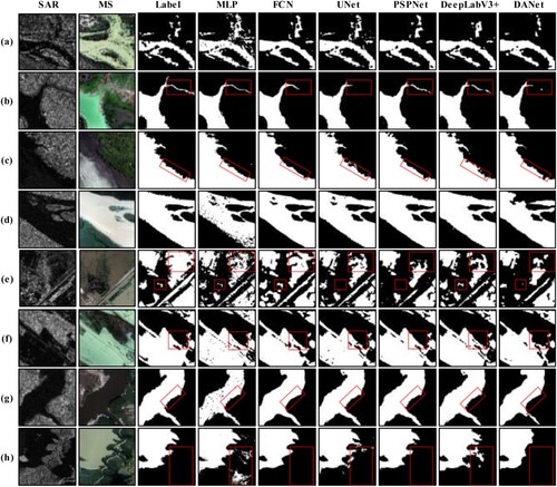
As shown in the qualitative results of Figure 6, all six models are competent for the flood area extraction task, even the simplest MLP can achieve good segmentation results. Although each model has some misclassifications, the extraction result is still acceptable. Specifically, with the support of the GF-FloodNet dataset in this paper, large rivers, lakes, etc. can be well extracted by the models, as shown in Figure 6(a,d,g). The models can accurately extract the edges of flood areas and effectively cope with the vague definition of flood area boundaries, although there is a partial loss of edge information caused by model structures such as FCN and DANet of Figure 6(c,f). Most of the detailed information can be detected, except that FCN, UNet, and DANet cannot extract the small tributaries shown in Figure 6(b). For the scattered small flood areas shown in Figure 6(e), the extraction results are incomplete. This is because the shallow flood depth and the easily confused boundary between the flood area and the bare land increase the difficulty of extraction. We could continue to augment similar samples to improve the effectiveness of our dataset for the extraction of small tributaries and scattered flood areas. For scenes with large undulating terrain, as shown in Figure 6(h), the models are more prone to misclassify the objects adjacent to the flood area. Therefore, we need more high-precision registered multi-source images containing flood areas to alleviate this phenomenon. For the spring flood caused by snowmelt shown in Figure 6(c,g), our dataset can also support the models to achieve good extraction results.

Figure 6. Visual comparison of flood area extraction results. Figure (a) - (h) show eight samples from the test set, along with labels and extraction results. The red boxes in the figure highlight the parts with significant differences between models.

From the above quantitative and qualitative analysis, benefiting from the GF-FloodNet dataset, different deep learning models achieve good performances in flood area extraction, as follows. (1) The GF-FloodNet dataset supports the training of models to extract large flood areas, including in spring flood scenarios containing ice or snow. (2) The trained models on our dataset can extract most of the detailed information, such as edge information and small tributaries, despite the slightly worse performance of some models. (3) The dataset facilitates the models to extract the scattered small flood areas. In short, the GF-FloodNet dataset has good support for training deep learning models to perform flood areas extraction well.

3.2.3. The site-specific effects on the deep learning models

For an intensive analysis of the site-specific effects on the deep learning models, we provide the MIoU, OA, and F1 for all models in each sampling region, as shown in Figure 7. The models show different advantages in different regions. Taking into account the characteristics of the sampling regions depicted in Figure 8, the analysis is as follows.

• In Brazil, Russia, and Russia Presoy, models trained on the GF-FloodNet dataset perform best. It indicates that these site-specific samples of our dataset improve the ability of the models to extract large contiguous flood areas in scenes with flat terrain and simple background.

• In South Africa, Pakistan, Australia, and India, the evaluation metrics become slightly worse, but the overall performance is still satisfactory. This shows that these site-specific samples are beneficial to models for feature learning in complex scenes. The models trained on such data can extract flood areas with diverse features, identify rich detail information, eliminate the interference of mountain shadows in undulating terrain areas, and cope with vague definition of flood area boundaries.

• In China, the models cannot learn features well and perform poorly due to the few training samples and the low image registration accuracy. While it may be difficult to completely avoid these problems, they can be improved by balancing the number of samples in each region.

Figure 7. Evaluation metrics for different models in each sampling region. (a) MIoU on the test set; (b) OA on the test set; (c) F1 on the test set.

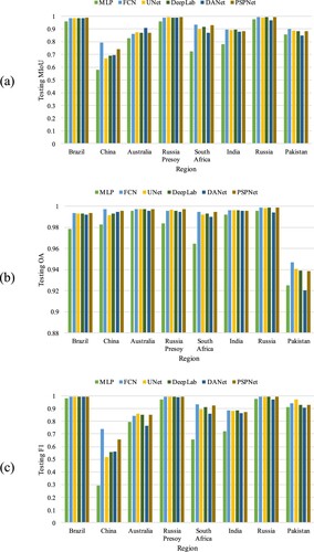
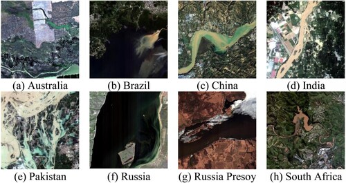
Figure 8. An example of the sampling regions. (a) Australia; (b) Brazil; (c) China; (d) India; (e) Pakistan; (f) Russia; (g) Russia Presoy; (h) South Africa. The regions such as Brazil, Russia, and Russia Presoy are dominated by large contiguous flood areas with flat terrain and simple backgrounds. The regions such as South Africa, Pakistan, Australia, and India have complex scenes such as variable characteristics of flood areas, undulating terrain, rich detail information, and vague definition of flood area boundaries. The regions such as China have few training samples and low image registration accuracy in the GF-FloodNet dataset.

It can be seen that the site-specific samples in the GF-FloodNet dataset have positive effects on deep learning models, which can help models learn a variety of valuable key features from them and extract flood areas effectively in diverse scenes.

3.2.4. Validation on large-scale remote sensing data

To validate whether the GF-FloodNet dataset can support deep learning models for extracting flood areas on large-scale remote sensing images, and the generalization of the model trained on our dataset, we carry out experiments in real scenes. We use additional multi-source images (MS-SAR) that are not involved in the GF-FloodNet dataset as real scene validation data. The images are from three topographically diverse regions, the Mekong Basin, the Pearl River Basin, and Venezuela, which suffered from floods. We collect validation data following the principle: the GF-3 SAR images containing flood events are first selected, and then the cloud-free GF-2 MS images from the same region are collected as auxiliary inputs. The data preprocessing is the same as before.

We use MLP, FCN, UNet, PSPNet, DeepLabV3+, and DANet trained on the GF-FloodNet dataset to extract flood areas from the three large-scale validation images. The results are shown in Figures 9–11.

Figure 9. Extraction results of the Mekong Basin. Figure (a) and Figure (b) represent two scene images from different regions of the Mekong Basin, respectively. The red boxes show the most obvious differences in the extraction results between models.

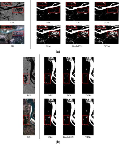
Figure 10. Extraction results of the Pearl River Basin. Figures (a) to (c) represent three different images of the Pearl River Basin. The red boxes show the most obvious differences in the extraction results between models.

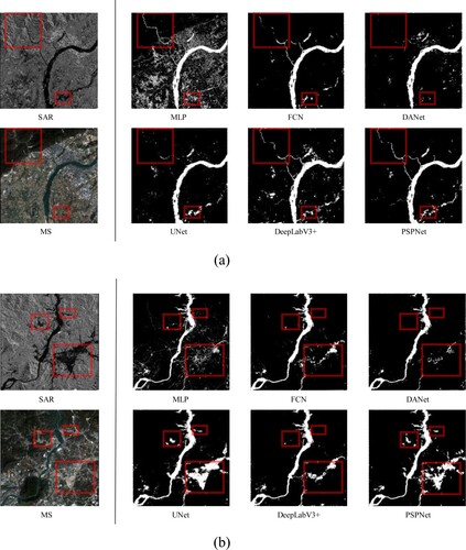
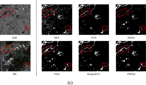
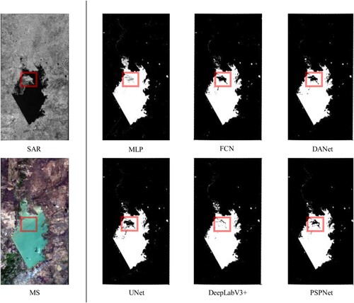
Figure 11. Extraction results of Venezuela. The red boxes show the most obvious differences in the extraction results between models.

In the Mekong Basin, as shown in Figure 9, the main flood areas are extracted, and the extraction for the mainstream of the river is relatively complete. For the red boxed areas in Figure 9(a), MLP, FCN, and DANet perform poorly, but UNet, PSPNet, and DeepLabV3 + can extract them better. For the small and irregular flood areas in Figure 9(b), none of the models can extract the entire area. This is mainly because these flood areas in the SAR image corresponding to the MS image are non-flood areas due to the difference in acquisition time, so the extraction is disturbed.

In the Pearl River Basin, as shown in Figure 10, most of the flood areas are well extracted by each model, even for the simplest MLP with many misclassifications of buildings and roads. For small tributaries and scattered small flood areas, different deep models diverge in the extraction results. They are influenced by both the complex background and the intrinsic structures of the models, as shown in the upper left corner of Figure 10(a). For multiple flood areas present only in SAR images but not in MS images, some models are confused in the extraction process, but UNet and PSPNet can well capture the key features in SAR images and achieve satisfactory results, as shown in the lower right corner of Figure 10(a) and the red boxes in Figure 10(b,c). If possible, this problem can be solved to a large extent by selecting MS reference images close to the time of the flood events. It is worth mentioning that, benefiting from the rich background and multi-source advantages of the GF-FloodNet dataset, mountain shadows in SAR images, which are most likely to interfere with flood area extraction, are well discriminated (only the simplest MLP cannot distinguish them).

In Venezuela, due to the simple background and flat terrain, the extraction results are visually good and relatively similar. The few differences lie in the red box region of Figure 11, which is also caused by the different categories in the same location of the MS and SAR images.

It is fully demonstrated that the deep learning models trained on the GF-FloodNet dataset achieve good generalization and can effectively extract flood areas on large-scale remote sensing images. This benefits from the diverse features of the site-specific samples, which promote the feature extraction and learning ability of the models in different flood scenes. Two examples are provided to understand the positive effects of site specific samples on the effectiveness and generalization of models.

• The samples from South Africa contain many mountain shadows in undulating terrain areas. The models trained on such data can effectively eliminate the interference of mountain shadows in the Pearl River Basin, such as shown in the red box at the upper left corner of Figure 10(a).

• The samples from Pakistan contain scattered small flood areas with irregularly shapes, increasing the difficulty of model extraction. Still, the trained models are capable of extracting similar features for flood area extraction in the Mekong River Basin, such as shown in the lower red box of Figure 9(a).

In Section 3.2, we present a comprehensive experimentation and analysis of the GF-FloodNet dataset from four different perspectives. The results indicate that the dataset can provide high-quality training samples for deep learning models to achieve satisfactory results in flood area extraction.

The GF-FloodNet dataset can serve as a baseline to evaluate the performance of different deep learning models fairly and reliably. This is because the difference in the extraction effect of flood areas depends on the different feature extraction capabilities of the models. The GF-FloodNet dataset contains site-specific samples from different regions spanning multiple climatic zones. Different natural environmental conditions form different topography and landforms, including mountains, plains, lakes, rivers, etc., so that the GF-FloodNet dataset covers a variety of common flood types, such as urban floods, mountain floods, and snowmelt spring floods, which are of great concern to us. The intra-class diversity of the dataset enables the models to learn key features from different flood scenes, and the extraction results can well reflect the differences between models. Thus, as a baseline with fairness and reliability, the GF-FloodNet dataset can be used for comparison and evaluation of common deep learning models in flood area extraction.

4. Discussion

4.1. Advantages of multi-source remote sensing data on the dataset

The proposed GF-FloodNet dataset has significant multi-source advantages. In order to clearly address how the multi-source data can improve the dataset quality and validate the advantages of multi-source data, we design comparative experiments based on different data sources.

4.1.1. Quantitative analysis based on evaluation metrics

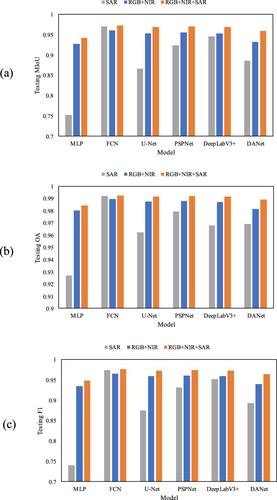
The single-channel (SAR) of GF-3 SAR, the 4-channel (RGB + NIR) of GF-2 MS, and the multi-source 5-channel (RGB + NIR + SAR) data are taken as different inputs for each model to compare the differences in model performance. We train the models with 100 epochs for each of the three types of inputs.

As shown in Figure 12, the models trained on RGB + NIR + SAR data achieve the best overall results, followed by the models trained on RGB + NIR data and the models trained on SAR data. This implies that multi-source data can improve the dataset quality compared to single-source datasets, as it supports the trained models to achieve better performance in the flood area extraction. Although only simple layer stacking is used, the combination of multiple sources can still show notable advantages and contribute to the high quality of the GF-FloodNet dataset.

Figure 12. Comparison results of each model trained on SAR, RGB + NIR, and RGB + NIR + SAR data. (a) MIoU on the test set; (b) OA on the test set; (c) F1 on the test set.

4.1.2. Qualitative analysis based on the interpretability with Grad-CAM

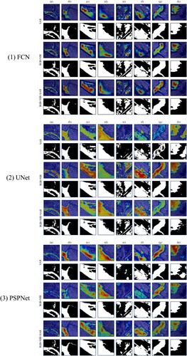
To better understand how multi-source data improves the quality of dataset, and further investigate what supporting roles multi-source data provides for the model training process compared to single-source, we conduct an interpretability analysis in this section. Specifically, we use Gradient-weighted Class Activation Mapping (Grad-CAM) to perform feature visualization on the models trained on SAR, RGB + NIR and RGB + NIR + SAR data. Since the simplest MLP does not contain convolutional layers to apply Grad-CAM, the experiments are only for FCN, UNet, PSPNet, DeepLabV3+, and DANet.

Figure 13 illustrates the feature visualization results of each model based on the Grad-CAM. The detailed analysis is as follows.

• For SAR inputs, the models have many missed detections or even fail to extract the flood areas at all, as shown in Figure 12-1(e) of DANet. Mountain shadows strongly interfere with the extraction performance of the models, as shown in Figure 12(h) of UNet, PSPNet, and DANet. Many details, including small tributaries, are not detected by the model, as shown in Figure 12(a,b) of each model.

• For RGB + NIR inputs, the results are much better than for SAR inputs. The rich spectral information of MS data helps the models to better focus on the features of flood areas. However, the edges of some results become blurred and there is an edge overflow phenomenon, as shown in Figure 12-4(g) of DeepLabV3 + and Figure 12-5(e) of DANet. This is because the focus of the models is distracted by the objects adjacent to the flood areas.

• For RGB + NIR + SAR inputs, multi-source data improve the models’ attention to flood areas, and the distribution of the focused areas is more concentrated and continuous. The inputs complement the advantages of MS images with SAR images, eliminate the interference of mountain shadows, and facilitate the model to extract more detailed information, including small tributaries, as shown in Figure 12-2(a) of UNet and Figure 12-3(b) of PSPNet. They also promote the models to better detect edge information and alleviate edge blurring and overflow phenomena.

Figure 13. Feature visualization results of each model based on Grad-CAM. In each heatmap, the red region is the most important, followed by orange and green, and the blue region is usually the least important region for the model.

The multi-source data improves the quality of GF-FloodNet dataset, which combines the advantages of MS and SAR data, provides more information for the models to better extract flood areas and overcomes the limitations of using a single data source. Specifically, the advantages of multi-source information are as follows.

• Compared with using only SAR data, multi-source data can reduce the interference of mountain shadows and detect more details such as small tributaries and scattered flood areas.

• Compared with using only MS data, multi-source data can distinguish neighboring objects with similar spectral information to the flood areas, and extract edges more accurately.

• Multi-source data improves dataset quality by combining the complementary advantages of MS and SAR data. It expands the availability and flexibility of the GF-FloodNet dataset, so that the dataset can be used for flood area extraction based on SAR, MS, or multi-source data in different actual needs.

Nevertheless, our utilization of multi-source data still presents certain shortcomings that require further improvement: (1) To ensure that the labels closely match the ground truth of each channel in multi-source data, the image registration accuracy needs to be improved in regions with large topographic undulations. (2) Advanced image fusion techniques (Liu et al. 2022) should be considered for flood area extraction using multi-source data. Because simple layer stacking may confuse the models when extracting flood areas.

In conclusion, the multi-source data improves the quality of our dataset, and supports the better training of several deep learning models to extract flood areas more effectively. The GF-FloodNet dataset has significant multi-source advantages and good application prospects.

4.2. Active learning versus random sampling

To verify the effectiveness of active learning in the construction of GF-FloodNet dataset, several experiments are designed for comparison. We adopt different query strategies, including random sampling, maximum entropy sampling, and least confidence sampling, and compare the MIoU for each model with the increasing proportion of labeled samples.

Specifically, in the initial stage, we randomly select 5% of the training dataset, i.e. 536 samples, and annotate them as initial training samples. After that, we select 5% of the training dataset according to the sample query strategy at each query, i.e. 536 candidate samples for labeling and participation in the training for 10 epochs. After each training iteration, all models are tested on the test dataset. In the active learning process, it takes 20 queries to annotate all the training samples. To ensure the fairness of the experiments, we use the same experimental environment and set the same random seeds for all models. The performance comparison of each group of experiments is shown in Figure 14. In the figure, p100 - 100epoch represents the testing MIoU of each model trained on all samples for 100 epochs, and p99 – 100epoch as the baseline represents 99% of the testing MIoU of each model trained on all samples for 100 epochs.

Figure 14. Variation curves of MIoU for each model based on different query strategies of active learning. The figure shows how the MIoU of each model changes as the percentage of labeled samples increases.

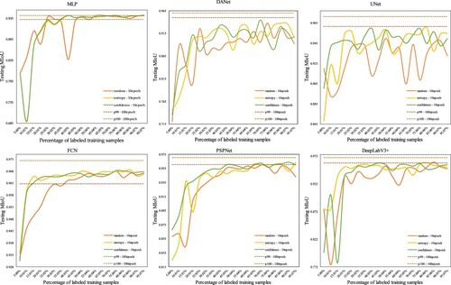
During the experiment, after the 9th iteration, the performance improvement of each model tends to slow down. The percentage of labeled training samples is about 45%, which can make the model performance very close to the highest MIoU acquired by training on all samples (the baseline p99 – 100epoch in Figure 14). It can be said that this can save about 55% of the annotation cost. Models based on maximum entropy sampling and least confidence sampling converge significantly faster than random sampling and can achieve higher model performance with the same number of training samples. As the percentage of labeled samples gradually increases, the testing MIoU of the models gradually improves. As the number of labeled samples continues to increase, the improvement of model performance tends to slow down. This is because the most uncertain samples have been labeled in the previous query process. When the subsequent less important samples are labeled, they cannot provide more information to the model that already achieved a good segmentation effect for flood and non-flood areas. Thus, the addition of the labeled samples in the later rounds does not significantly improve the overall performance of the model.

In summary, the sample selection strategy based on active learning in this paper is feasible and applicable to different model structures. Through the strategy, we effectively select the most valuable samples from the unlabeled samples pool and construct the GF-FloodNet dataset. The effectiveness of the dataset can be well verified again.

4.3. How many samples on earth are sufficient for the flood area extraction

As mentioned above, the annotation of remote sensing data is very costly. It is generally believed that in deep learning more training samples are better for the model to improve its performance, although they may add a lot of unnecessary data annotation costs and cause redundancy. Therefore, it would be good if we can train the model with as few samples as possible to achieve good results, which is our original intention to construct the dataset using active learning. In this section, we discuss the boundary of the GF-FloodNet dataset as well as how many GF 3–2 training samples we need on earth are sufficient for the flood extraction task.

From the analysis in the previous section, we know that when the labeled training samples reach about 45% of the total training samples, i.e. when the model is trained on 4824 training samples for 10 epochs, all models have reached relatively good performance and the subsequent improvement starts to slow down. Therefore, we assume that 4824 training samples of 256 × 256 pixels from GF 3–2 can be sufficient for flood area extraction.

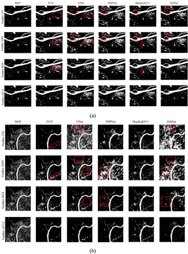
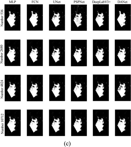
To further verify our conjecture, investigate the effect of different number of training samples on the model performance, and explore the boundary of the dataset, we train six deep models based on 5% (536 samples), 25% (2680 samples), 45% (4824 samples), and 100% (10712 samples) of the training dataset with 100 epochs. In order to reduce the variation of the model performance due to the randomness of dataset division and sample distribution, we adopt a dynamic cross-validation during the experiments. The training set, validation set, and test set are divided by setting k different random seeds (k = 5) to change their internal sample distribution. We compute the means and standard deviations of evaluation metrics over all the k seeds as the final testing results of each model. The testing results of the models based on the different number of training samples are shown in Figure 15. The results of flood area extraction in large-scale remote sensing images are shown in Figure 16.

Figure 15. Testing results of models based on the different number of training samples. (a) MIoU on the test set; (b) OA on the test set; (c) F1 on the test set. The figure shows the average performance of the model over k random experiments with different number of training samples.

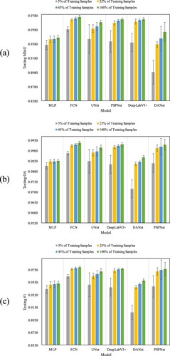
Figure 16. Results of flood area extraction in large-scale remote sensing images. (a) The Mekong Basin. (b) The Pearl River Basin. (c) Venezuela. The figure shows the extraction results of each model based on different number of training samples in three regions. The red boxes show the areas where we focus on for comparison.

As the number of training samples increases in Figure 15, the evaluation metrics of each model show an overall increasing trend. MIoU, as an important evaluation metric for flood area extraction, increases the most.

Specifically, for the percentage of training samples from 5% (536 samples) to 25% (2680 samples), the increase of each model’s metrics reach the highest. The increase for MIoU of MLP, FCN, UNet, PSPNet, DeepLabV3+, and DANet reach 0.79%, 1.36%, 1.48%, 2.62%, 2.95%, and 3.88%, respectively. The standard deviation of each model also becomes significantly smaller, which indicates that the model performance is more stable. This is also reflected in the visualization results, where the MLP predictions don’t change much, but the other models improve significantly, with fewer missed detections, and more flood area extractions. Most importantly, the interference of mountain shadows is greatly reduced, mainly as shown in the results of UNet and DANet in Figure 16(b).

From 25% (2680 samples) to 45% (4824 samples), the growth of the evaluation metrics decrease significantly, but the overall evaluation metrics of the models are still increasing. The lowest MIoU increase of 0.01% is achieved by MLP, and the highest is achieved by DANet with an increase of 0.84%. The overall standard deviation of each model’s MIoU is still relatively low and similar to the previous levels, although the standard deviation of DANet has increased. The models have already performed well when trained on these 4824 samples and became relatively stable. As reflected in the visualization results, the model extraction results continue to improve and become more in line with human visual interpretation.

From 45% (4824 samples) to 100% (10712 samples), the evaluation metrics continue to increase, and the growth remains small. The standard deviation of each model is still low, and the reduction is not significant. The performance of these models has not changed much. As shown in the visualization results, UNet, PSPNet, and DeepLabV3 + continue to improve. Instead, FCN and DANet behave worse, missing some of the flood areas that could be extracted in the previous stages, as shown in the fourth row of Figure 16(b) for FCN and DANet. The reasons seem to be twofold. One is that this part of the flood area exists only in the SAR image, while the reference cloud-free MS image has no flood at the same location. The other is that the models we use rely only on layer stacking when trained on multi-source data, without introducing any image fusion technology, so it causes the models to become so confused when extracting flood areas that they make incorrect judgments.

Furthermore, it is evident that the model performance is significantly influenced by the topographic features in the regions of remote sensing images. As shown in Figure 16, for regions with complex topography and diverse background objects, such as mountainous areas and urban areas in the Pearl River Basin, increasing the number of training samples will significantly improve the model performances and better eliminate the interference caused by background objects. For regions with flat terrain and simple background objects, such as the Mekong River Basin and Venezuela, increasing the number of training samples will have less impact. Even models trained with less than 4824 samples can achieve good results. In other words, the specific number of training samples can be determined according to the actual application requirements and time constraints of different tasks.

In summary, for the multi-source remote sensing data consisting of GF-3 SAR images and GF-2 MS images, we consider that 4824 training samples are sufficient for training most models to achieve acceptable good flood area extraction results no matter how the training set, validation set, and test set are divided. For sample datasets in deep learning, there should be a potential optimal boundary for the model to achieve excellent performance, where the model performance no longer improves significantly even if the number of training samples continues to increase. In the GF-FloodNet dataset, the number of 4824 training samples is relatively close to this boundary value. Other datasets can also refer to our viewpoint during the dataset construction and model training process, thus reducing the annotation cost and improving the training efficiency to some extent.

5. Conclusions

In this paper, we propose a new multi-source remote sensing image sample dataset with high resolution for flood area extraction called GF-FloodNet. The construction process uses a multi-level sample selection and semi-automatic interactive annotation strategy based on active learning. The dataset consists of GF-3 and GF-2 satellite images with a maximum resolution of 1.5 m and contains 13,388 samples with pixel-level labels stored in TIFF format.

Based on the GF-FloodNet dataset, we train different deep learning models for flood area extraction and conduct in-depth analysis and discussion. The results reveal that:

1. The GF-FloodNet dataset has high quality and significant advantages mainly due to the multi-source images, which combines rich spectral information of MS images with the ability of SAR sensors to penetrate through clouds.

2. The dataset construction based on active learning not only reduces the annotation cost but also improves the performance of deep learning models.

3. The models trained on the site-specific samples of GF-FloodNet dataset has good generalization and can be effectively applied to flood area extraction on large-scale remote sensing images of real scenes.

4. For any deep learning sample datasets, there should be a potential optimal boundary where the model can be trained on as few samples as possible to achieve good performance. The boundary of the GF-FloodNet seems close to 4824 training samples.

In conclusion, the GF-FloodNet dataset has various advantages such as multiple sampling regions, multi-source data advantages, rich intra-class diversity, and high spatial resolution. It can provide high-quality training samples for deep learning models to effectively extract flood areas. The trained models can be applied to large-scale remote sensing images, which reflects the application value of the GF-FloodNet dataset.

In the future, we will continue to extend the GF-FloodNet dataset with more advanced methods to incorporate more diverse and valuable samples. We hope that our dataset can contribute to the development of intelligent remote sensing flood monitoring.

Acknowledgments

This work was supported by the National Natural Science Foundation of China (No. U2243222, No. 42071413, and No. 41971397). We thank the editors and the anonymous reviewers for their valuable comments to improve the quality of this manuscript.

Disclosure statement

No potential conflict of interest was reported by the author(s).

Data availability statement

The GF-FloodNet dataset is publicly available at https://www.kaggle.com/datasets/pengliuair/gf-floodnet and https://pan.baidu.com/s/11yx5ERsGkkfUQXPYn34KkQ?pwd = yh47.

Correction Statement

This article was originally published with errors, which have now been corrected in the online version. Please see Correction (http://dx.doi.org/10.1080/17538947.2023.2238962).

Additional information

Funding

This work was supported by the National Natural Science Foundation of China under Grant number U2243222, 42071413, and 41971397.

References

- Amitrano, Donato, Gerardo Di Martino, Antonio Iodice, Daniele Riccio, and Giuseppe Ruello. 2018. “Unsupervised Rapid Flood Mapping Using Sentinel-1 GRD SAR Images.” IEEE Transactions on Geoscience and Remote Sensing 56 (6): 3290–3299. https://doi.org/10.1109/TGRS.2018.2797536.
- Anusha, N., and B. Bharathi. 2020. “Flood Detection and Flood Mapping Using Multi-Temporal Synthetic Aperture Radar and Optical Data.” The Egyptian Journal of Remote Sensing and Space Science 23 (2): 207–219. https://doi.org/10.1016/j.ejrs.2019.01.001.
- Bai, Yanbing, Wenqi Wu, Zhengxin Yang, Jinze Yu, Bo Zhao, Xing Liu, Hanfang Yang, Erick Mas, and Shunichi Koshimura. 2021. “Enhancement of Detecting Permanent Water and Temporary Water in Flood Disasters by Fusing Sentinel-1 and Sentinel-2 Imagery Using Deep Learning Algorithms: Demonstration of sen1floods11 Benchmark Datasets.” Remote Sensing 13 (11): 2220. https://doi.org/10.3390/rs13112220.
- Belharbi, Soufiane, Ismail Ben Ayed, Luke McCaffrey, and Eric Granger. 2021. “Deep active learning for joint classification & segmentation with weak annotator.” Paper presented at the Proceedings of the IEEE/CVF Winter Conference on Applications of Computer Vision.
- Beluch, William H, Tim Genewein, Andreas Nürnberger, and Jan M Köhler. 2018. “The Power of Ensembles for Active Learning in Image Classification.” Paper Presented at the Proceedings of the IEEE Conference on Computer Vision and Pattern Recognition.
- Benoudjit, Abdelhakim, and Raffaella Guida. 2019. “A Novel Fully Automated Mapping of the Flood Extent on SAR Images Using a Supervised Classifier.” Remote Sensing 11 (7): 779. https://doi.org/10.3390/rs11070779.
- Bischke, Benjamin, Patrick Helber, Simon Brugman, Erkan Basar, Zhengyu Zhao, Martha A Larson, and Konstantin Pogorelov. 2019. “The Multimedia Satellite Task at MediaEval 2019.” Paper Presented at the MediaEval.
- Bonafilia, Derrick, Beth Tellman, Tyler Anderson, and Erica Issenberg. 2020. “Sen1Floods11: A Georeferenced Dataset to Train and Test Deep Learning Flood Algorithms for Sentinel-1.” Paper Presented at the Proceedings of the IEEE/CVF Conference on Computer Vision and Pattern Recognition Workshops.
- Chen, Liang-Chieh, Yukun Zhu, George Papandreou, Florian Schroff, and Hartwig Adam. 2018. “Encoder-decoder with Atrous Separable Convolution for Semantic Image Segmentation.” Paper Presented at the Proceedings of the European Conference on Computer Vision (ECCV).
- Chowdhury, Tashnim, and Maryam Rahnemoonfar. 2021. “Attention Based Semantic Segmentation on UAV Dataset for Natural Disaster Damage Assessment.” Paper Presented at the 2021 IEEE International Geoscience and Remote Sensing Symposium IGARSS.
- Desai, Shasvat, and Debasmita Ghose. 2022. “Active Learning for Improved Semi-Supervised Semantic Segmentation in Satellite Images.” Paper presented at the Proceedings of the IEEE/CVF Winter Conference on Applications of Computer Vision.
- Drakonakis, Georgios I, Grigorios Tsagkatakis, Konstantina Fotiadou, and Panagiotis Tsakalides. 2022. “Ombrianet—Supervised Flood Mapping via Convolutional Neural Networks Using Multitemporal Sentinel-1 and Sentinel-2 Data Fusion.” IEEE Journal of Selected Topics in Applied Earth Observations and Remote Sensing 15: 2341–2356. https://doi.org/10.1109/JSTARS.2022.3155559.
- Feng, Wenqing, Haigang Sui, Weiming Huang, Chuan Xu, and Kaiqiang An. 2019. “Water Body Extraction from Very High-Resolution Remote Sensing Imagery Using Deep U-Net and a Superpixel-Based Conditional Random Field Model.” IEEE Geoscience and Remote Sensing Letters 16 (4): 618–622. https://doi.org/10.1109/LGRS.2018.2879492.
- Fu, Jun, Jing Liu, Haijie Tian, Yong Li, Yongjun Bao, Zhiwei Fang, and Hanqing Lu. 2019. “Dual Attention Network for Scene Segmentation.” Paper Presented at the Proceedings of the IEEE/CVF Conference on Computer Vision and Pattern Recognition.
- Goffi, Alessia, Daniela Stroppiana, Pietro Alessandro Brivio, Gloria Bordogna, and Mirco Boschetti. 2020. “Towards an Automated Approach to map Flooded Areas from Sentinel-2 MSI Data and Soft Integration of Water Spectral Features.” International Journal of Applied Earth Observation and Geoinformation 84: 101951. https://doi.org/10.1016/j.jag.2019.101951.
- Gorriz, Marc, Axel Carlier, Emmanuel Faure, and Xavier Giro-i-Nieto. 2017. “Cost-effective Active Learning for Melanoma Segmentation.” arXiv preprint arXiv:1711.09168.
- Hamidi, Ebrahim, Brad G Peter, David F Muñoz, Hamed Moftakhari, and Hamid Moradkhani. 2023. “Fast Flood Extent Monitoring With SAR Change Detection Using Google Earth Engine.” IEEE Transactions on Geoscience and Remote Sensing 61: 1–19. https://doi.org/10.1109/TGRS.2023.3240097.
- He, Xiaoning, Shuangcheng Zhang, Bowei Xue, Tong Zhao, and Tong Wu. 2023. “Cross-modal Change Detection Flood Extraction Based on Convolutional Neural Network.” International Journal of Applied Earth Observation and Geoinformation 117: 103197. https://doi.org/10.1016/j.jag.2023.103197.
- Jiang, Xin, Shijing Liang, Xinyue He, Alan D Ziegler, Peirong Lin, Ming Pan, Dashan Wang, Junyu Zou, Dalei Hao, and Ganquan Mao. 2021. “Rapid and Large-Scale Mapping of Flood Inundation via Integrating Spaceborne Synthetic Aperture Radar Imagery with Unsupervised Deep Learning.” ISPRS Journal of Photogrammetry and Remote Sensing 178: 36–50. https://doi.org/10.1016/j.isprsjprs.2021.05.019.
- Joshi, Ajay J, Fatih Porikli, and Nikolaos Papanikolopoulos. 2009. “Multi-class active learning for image classification.” Paper presented at the 2009 IEEE conference on computer vision and pattern recognition.
- Konapala, Goutam, Sujay V Kumar, and Shahryar Khalique Ahmad. 2021. “Exploring Sentinel-1 and Sentinel-2 Diversity for Flood Inundation Mapping Using Deep Learning.” ISPRS Journal of Photogrammetry and Remote Sensing 180: 163–173. https://doi.org/10.1016/j.isprsjprs.2021.08.016.
- Kool, Juliette, Stef Lhermitte, Markus Hrachowitz, Francesco Bregoli, and Michael E McClain. 2022. “Seasonal Inundation Dynamics and Water Balance of the Mara Wetland, Tanzania Based on Multi-Temporal Sentinel-2 Image Classification.” International Journal of Applied Earth Observation and Geoinformation 109: 102766. https://doi.org/10.1016/j.jag.2022.102766.
- Lei, Zhao, Yi Zeng, Peng Liu, and Xiaohui Su. 2021. “Active Deep Learning for Hyperspectral Image Classification with Uncertainty Learning.” IEEE Geoscience and Remote Sensing Letters 19: 1–5.
- Lenczner, Gaston, Adrien Chan-Hon-Tong, Bertrand Le Saux, Nicola Luminari, and Guy Le Besnerais. 2022. “DIAL: Deep Interactive and Active Learning for Semantic Segmentation in Remote Sensing.” IEEE Journal of Selected Topics in Applied Earth Observations and Remote Sensing 15: 3376–3389. https://doi.org/10.1109/JSTARS.2022.3166551.
- Li, Zhouyayan, and Ibrahim Demir. 2023. “U-net-based Semantic Classification for Flood Extent Extraction Using SAR Imagery and GEE Platform: A Case Study for 2019 Central US Flooding.” Science of The Total Environment 869: 161757. https://doi.org/10.1016/j.scitotenv.2023.161757.
- Li, Wenning, Yi Li, Jianhua Gong, Quanlong Feng, Jieping Zhou, Jun Sun, Chenhui Shi, and Weidong Hu. 2021. “Urban Water Extraction with UAV High-Resolution Remote Sensing Data Based on an Improved U-Net Model.” Remote Sensing 13 (16): 3165. https://doi.org/10.3390/rs13163165.
- Li, Ziyao, Rui Wang, Wen Zhang, Fengmin Hu, and Lingkui Meng. 2019. “Multiscale Features Supported DeepLabV3+ Optimization Scheme for Accurate Water Semantic Segmentation.” IEEE Access 7: 155787–155804. https://doi.org/10.1109/ACCESS.2019.2949635.
- Liang, Jiayong, and Desheng Liu. 2020. “A Local Thresholding Approach to Flood Water Delineation Using Sentinel-1 SAR Imagery.” ISPRS Journal of Photogrammetry and Remote Sensing 159: 53–62. https://doi.org/10.1016/j.isprsjprs.2019.10.017.
- Liu, Peng, Jun Li, Lizhe Wang, and Guojin He. 2022. “Remote Sensing Data Fusion with Generative Adversarial Networks: State-of-the-art Methods and Future Research Directions.” IEEE Geoscience and Remote Sensing Magazine 10 (2): 295–328. https://doi.org/10.1109/MGRS.2022.3165967.
- Liu, Peng, Lizhe Wang, Rajiv Ranjan, Guojin He, and Lei Zhao. 2022. “Deep Learning for Anomaly Detection.” ACM Computing Surveys 54 (10s): 1–38. https://doi.org/10.1145/3439950.
- Liu, Peng, Hui Zhang, and Kie B Eom. 2016. “Active Deep Learning for Classification of Hyperspectral Images.” IEEE Journal of Selected Topics in Applied Earth Observations and Remote Sensing 10 (2): 712–724.
- Long, Jonathan, Evan Shelhamer, and Trevor Darrell. 2015. “Fully Convolutional Networks for Semantic Segmentation.” Paper Presented at the Proceedings of the IEEE Conference on Computer Vision and Pattern Recognition.
- Mackowiak, Radek, Philip Lenz, Omair Ghori, Ferran Diego, Oliver Lange, and Carsten Rother. 2018. “Cereals-Cost-Effective Region-Based Active Learning for Semantic Segmentation.” arXiv preprint arXiv:1810.09726.
- Mahapatra, Dwarikanath, Behzad Bozorgtabar, Jean-Philippe Thiran, and Mauricio Reyes. 2018. “Efficient Active Learning for Image Classification and Segmentation Using a Sample Selection and Conditional Generative Adversarial Network.” Paper Presented at the Medical Image Computing and Computer Assisted Intervention–MICCAI 2018: 21st International Conference, Granada, Spain, September 16-20, 2018, Proceedings, Part II 11.
- Manakos, Ioannis, Georgios A Kordelas, and Kalliroi Marini. 2020. “Fusion of Sentinel-1 Data with Sentinel-2 Products to Overcome non-Favourable Atmospheric Conditions for the Delineation of Inundation Maps.” European Journal of Remote Sensing 53 (sup2): 53–66. https://doi.org/10.1080/22797254.2019.1596757.
- Martinis, Sandro, Jens Kersten, and André Twele. 2015. “A Fully Automated TerraSAR-X Based Flood Service.” ISPRS Journal of Photogrammetry and Remote Sensing 104: 203–212. https://doi.org/10.1016/j.isprsjprs.2014.07.014.
- Martinis, Sandro, Simon Plank, and Kamila Ćwik. 2018. “The use of Sentinel-1 Time-Series Data to Improve Flood Monitoring in Arid Areas.” Remote Sensing 10 (4): 583. https://doi.org/10.3390/rs10040583.
- Martinis, Sandro, André Twele, and Stefan Voigt. 2009. “Towards Operational Near Real-Time Flood Detection Using a Split-Based Automatic Thresholding Procedure on High Resolution TerraSAR-X Data.” Natural Hazards and Earth System Sciences 9 (2): 303–314. https://doi.org/10.5194/nhess-9-303-2009.
- Mason, David C, Ian J Davenport, Jeffrey C Neal, Guy J-P Schumann, and Paul D Bates. 2012. “Near Real-Time Flood Detection in Urban and Rural Areas Using High-Resolution Synthetic Aperture Radar Images.” IEEE Transactions on Geoscience and Remote Sensing 50 (8): 3041–3052. https://doi.org/10.1109/TGRS.2011.2178030.
- Mateo-Garcia, Gonzalo, Joshua Veitch-Michaelis, Lewis Smith, Silviu Vlad Oprea, Guy Schumann, Yarin Gal, Atılım Güneş Baydin, and Dietmar Backes. 2021. “Plasma Hsp90 Levels in Patients with Systemic Sclerosis and Relation to Lung and Skin Involvement: A Cross-Sectional and Longitudinal Study.” Scientific Reports 11 (1): 1–12. https://doi.org/10.1038/s41598-020-79139-8.
- Matiz, Sergio, and Kenneth E Barner. 2019. “Inductive Conformal Predictor for Convolutional Neural Networks: Applications to Active Learning for Image Classification.” Pattern Recognition 90: 172–182. https://doi.org/10.1016/j.patcog.2019.01.035.
- Nemni, Edoardo, Joseph Bullock, Samir Belabbes, and Lars Bromley. 2020. “Fully Convolutional Neural Network for Rapid Flood Segmentation in Synthetic Aperture Radar Imagery.” Remote Sensing 12 (16): 2532. https://doi.org/10.3390/rs12162532.
- Ouled Sghaier, Moslem, Imen Hammami, Samuel Foucher, and Richard Lepage. 2018. “Flood Extent Mapping from Time-Series SAR Images Based on Texture Analysis and Data Fusion.” Remote Sensing 10 (2): 237. https://doi.org/10.3390/rs10020237.
- Ozdemir, Firat, Zixuan Peng, Philipp Fuernstahl, Christine Tanner, and Orcun Goksel. 2021. “Active Learning for Segmentation Based on Bayesian Sample Queries.” Knowledge-Based Systems 214: 106531. https://doi.org/10.1016/j.knosys.2020.106531.
- Pradhan, Biswajeet, Ulrike Hagemann, Mahyat Shafapour Tehrany, and Nikolas Prechtel. 2014. “An Easy to use ArcMap Based Texture Analysis Program for Extraction of Flooded Areas from TerraSAR-X Satellite Image.” Computers & Geosciences 63: 34–43. https://doi.org/10.1016/j.cageo.2013.10.011.
- Qin, Peng, Yulin Cai, and Xueli Wang. 2021. “Small Waterbody Extraction with Improved U-Net Using Zhuhai-1 Hyperspectral Remote Sensing Images.” IEEE Geoscience and Remote Sensing Letters 19: 1–5.
- Rahnemoonfar, Maryam, Tashnim Chowdhury, Argho Sarkar, Debvrat Varshney, Masoud Yari, and Robin Roberson Murphy. 2021. “Floodnet: A High Resolution Aerial Imagery Dataset for Post Flood Scene Understanding.” IEEE Access 9: 89644–89654. https://doi.org/10.1109/ACCESS.2021.3090981.
- Rambour, Clément, Nicolas Audebert, E. Koeniguer, Bertrand Le Saux, M. Crucianu, and Mihai Datcu. 2020. “Flood Detection in Time Series of Optical and sar Images.” The International Archives of the Photogrammetry, Remote Sensing and Spatial Information Sciences XLIII-B2-2020 (B2): 1343–1346. https://doi.org/10.5194/isprs-archives-XLIII-B2-2020-1343-2020.
- Rangnekar, Aneesh, Christopher Kanan, and Matthew Hoffman. 2023. “Semantic Segmentation with Active Semi-Supervised Learning.” Paper presented at the Proceedings of the IEEE/CVF Winter Conference on Applications of Computer Vision.
- Rentschler, Jun, Melda Salhab, and Bramka Arga Jafino. 2022. “Flood Exposure and Poverty in 188 Countries.” Nature Communications 13 (1): 3527. https://doi.org/10.1038/s41467-022-30727-4.
- Ronneberger, Olaf, Philipp Fischer, and Thomas Brox. 2015. “U-net: Convolutional Networks for Biomedical Image Segmentation.” Paper Presented at the Medical Image Computing and Computer-Assisted Intervention–MICCAI 2015: 18th International Conference, Munich, Germany, October 5-9, 2015, Proceedings, Part III 18.
- Ruiz, Pablo, Javier Mateos, Gustavo Camps-Valls, Rafael Molina, and Aggelos K Katsaggelos. 2014. “Bayesian Active Remote Sensing Image Classification.” IEEE Transactions on Geoscience and Remote Sensing 52 (4): 2186–2196. https://doi.org/10.1109/TGRS.2013.2258468.
- Rumelhart, David E., Geoffrey E. Hinton, and Ronald J. Williams. 1986. “Learning Representations by Back-Propagating Errors.” Nature 323: 533–536. https://doi.org/10.1038/323533a0.
- Saidu, Isah Charles, and Lehel Csató. 2021. “Active Learning with Bayesian UNet for Efficient Semantic Image Segmentation.” Journal of Imaging 7 (2): 37. https://doi.org/10.3390/jimaging7020037.
- Senthilnath, J., H. Vikram Shenoy, Ritwik Rajendra, S. N. Omkar, V. Mani, and P. G. Diwakar. 2013. “Integration of Speckle de-Noising and Image Segmentation Using Synthetic Aperture Radar Image for Flood Extent Extraction.” Journal of Earth System Science 122: 559–572. https://doi.org/10.1007/s12040-013-0305-z.
- Singha, Mrinal, Jinwei Dong, Sangeeta Sarmah, Nanshan You, Yan Zhou, Geli Zhang, Russell Doughty, and Xiangming Xiao. 2020. “Identifying Floods and Flood-Affected Paddy Rice Fields in Bangladesh Based on Sentinel-1 Imagery and Google Earth Engine.” ISPRS Journal of Photogrammetry and Remote Sensing 166: 278–293. https://doi.org/10.1016/j.isprsjprs.2020.06.011.
- Sinha, Samarth, Sayna Ebrahimi, and Trevor Darrell. 2019. “Variational Adversarial Active Learning.” Paper Presented at the Proceedings of the IEEE/CVF International Conference on Computer Vision.
- Slagter, Bart, Nandin-Erdene Tsendbazar, Andreas Vollrath, and Johannes Reiche. 2020. “Mapping Wetland Characteristics Using Temporally Dense Sentinel-1 and Sentinel-2 Data: A Case Study in the St. Lucia Wetlands, South Africa.” International Journal of Applied Earth Observation and Geoinformation 86: 102009. https://doi.org/10.1016/j.jag.2019.102009.
- Son, Nguyen-Thanh, Chi-Farn Chen, and Cheng-Ru Chen. 2021. “Flood Assessment Using Multi-Temporal Remotely Sensed Data in Cambodia.” Geocarto International 36 (9): 1044–1059. https://doi.org/10.1080/10106049.2019.1633420.
- Sourati, Jamshid, Ali Gholipour, Jennifer G Dy, Xavier Tomas-Fernandez, Sila Kurugol, and Simon K Warfield. 2019. “Intelligent Labeling Based on Fisher Information for Medical Image Segmentation Using Deep Learning.” IEEE Transactions on Medical Imaging 38 (11): 2642–2653. https://doi.org/10.1109/TMI.2019.2907805.
- Tavus, Beste, Sultan Kocaman, and Candan Gokceoglu. 2022. “Flood Damage Assessment with Sentinel-1 and Sentinel-2 Data After Sardoba dam Break with GLCM Features and Random Forest Method.” Science of The Total Environment 816: 151585. https://doi.org/10.1016/j.scitotenv.2021.151585.
- Tavus, B., S. Kocaman, H. A. Nefeslioglu, and C. Gokceoglu. 2020. “A Fusion Approach for Flood Mapping Using Sentinel-1 and Sentinel-2 Datasets.” The International Archives of the Photogrammetry, Remote Sensing and Spatial Information Sciences 43: 641–648.
- Tellman, B., J. A. Sullivan, C. Kuhn, A. J. Kettner, C. S. Doyle, G. R. Brakenridge, T. A. Erickson, and D. A. Slayback. 2021. “Satellite Imaging Reveals Increased Proportion of Population Exposed to Floods.” Nature 596 (7870): 80–86. https://doi.org/10.1038/s41586-021-03695-w.
- Tiwari, Varun, Vinay Kumar, Mir Abdul Matin, Amrit Thapa, Walter Lee Ellenburg, Nishikant Gupta, and Sunil Thapa. 2020. “Flood Inundation Mapping-Kerala 2018; Harnessing the Power of SAR, Automatic Threshold Detection Method and Google Earth Engine.” PLoS One 15 (8): e0237324.
- Tralli, David M, Ronald G Blom, Victor Zlotnicki, Andrea Donnellan, and Diane L Evans. 2005. “Satellite Remote Sensing of Earthquake, Volcano, Flood, Landslide and Coastal Inundation Hazards.” ISPRS Journal of Photogrammetry and Remote Sensing 59 (4): 185–198. https://doi.org/10.1016/j.isprsjprs.2005.02.002.
- Tuia, Devis, Michele Volpi, Loris Copa, Mikhail Kanevski, and Jordi Munoz-Mari. 2011. “A Survey of Active Learning Algorithms for Supervised Remote Sensing Image Classification.” IEEE Journal of Selected Topics in Signal Processing 5 (3): 606–617. https://doi.org/10.1109/JSTSP.2011.2139193.
- Twele, André, Wenxi Cao, Simon Plank, and Sandro Martinis. 2016. “Sentinel-1-based Flood Mapping: A Fully Automated Processing Chain.” International Journal of Remote Sensing 37 (13): 2990–3004. https://doi.org/10.1080/01431161.2016.1192304.
- Vanama, V. S. K., Y. S. Rao, and C. M. Bhatt. 2021. “Change Detection Based Flood Mapping Using Multi-Temporal Earth Observation Satellite Images: 2018 Flood Event of Kerala, India.” European Journal of Remote Sensing 54 (1): 42–58. https://doi.org/10.1080/22797254.2020.1867901.
- Wang, Bin, Zhanlong Chen, Liang Wu, Xiaohong Yang, and Yuan Zhou. 2022. “SADA-net: A Shape Feature Optimization and Multiscale Context Information-Based Water Body Extraction Method for High-Resolution Remote Sensing Images.” IEEE Journal of Selected Topics in Applied Earth Observations and Remote Sensing 15: 1744–1759. https://doi.org/10.1109/JSTARS.2022.3146275.
- Wang, Ruo-Qian, and Yangmin Ding. 2022. “Semi-supervised identification and mapping of surface water extent using street-level monitoring videos.” Big Earth Data, 1–19.
- Wang, Jingming, Shixin Wang, Futao Wang, Yi Zhou, Zhenqing Wang, Jianwan Ji, Yibing Xiong, and Qing Zhao. 2022. “FWENet: A Deep Convolutional Neural Network for Flood Water Body Extraction Based on SAR Images.” International Journal of Digital Earth 15 (1): 345–361. https://doi.org/10.1080/17538947.2021.1995513.
- Wang, Peng, Gong Zhang, and Henry Leung. 2019. “Improving Super-Resolution Flood Inundation Mapping for Multispectral Remote Sensing Image by Supplying More Spectral Information.” IEEE Geoscience and Remote Sensing Letters 16 (5): 771–775. https://doi.org/10.1109/LGRS.2018.2882516.
- Yang, Lin, Yizhe Zhang, Jianxu Chen, Siyuan Zhang, and Danny Z Chen. 2017. “Suggestive Annotation: A Deep Active Learning Framework for Biomedical Image Segmentation.” Paper Presented at the Medical Image Computing and Computer Assisted Intervention− MICCAI 2017: 20th International Conference, Quebec City, QC, Canada, September 11-13, 2017, Proceedings, Part III 20.
- Yuan, Jin, Xingxing Hou, Yaoqiang Xiao, Da Cao, Weili Guan, and Liqiang Nie. 2019. “Multi-criteria Active Deep Learning for Image Classification.” Knowledge-Based Systems 172: 86–94. https://doi.org/10.1016/j.knosys.2019.02.013.
- Zhao, Hengshuang, Jianping Shi, Xiaojuan Qi, Xiaogang Wang, and Jiaya Jia. 2017. “Pyramid Scene Parsing Network.” Paper Presented at the Proceedings of the IEEE Conference on Computer Vision and Pattern Recognition.
- Zhao, Bofei, Haigang Sui, and Junyi Liu. 2023. “Siam-DWENet: Flood Inundation Detection for SAR Imagery Using a Cross-Task Transfer Siamese Network.” International Journal of Applied Earth Observation and Geoinformation 116: 103132. https://doi.org/10.1016/j.jag.2022.103132.