Adopting GPU computing to support DL-based Earth science applications

ABSTRACT

With the advancement of Artificial Intelligence (AI) technologies and accumulation of big Earth data, Deep Learning (DL) has become an important method to discover patterns and understand Earth science processes in the past several years. While successful in many Earth science areas, AI/DL applications are often challenging for computing devices. In recent years, Graphics Processing Unit (GPU) devices have been leveraged to speed up AI/DL applications, yet computational performance still poses a major barrier for DL-based Earth science applications. To address these computational challenges, we selected five existing sample Earth science AI applications, revised the DL-based models/algorithms, and tested the performance of multiple GPU computing platforms to support the applications. Application software packages, performance comparisons across different platforms, along with other results, are summarized. This article can help understand how various AI/ML Earth science applications can be supported by GPU computing and help researchers in the Earth science domain better adopt GPU computing (such as supermicro, GPU clusters, and cloud computing-based) for their AI/ML applications, and to optimize their science applications to better leverage the computing device.

KEYWORDS:

• GPU computing
• GeoAI
• open science
• Earth science
• artificial intelligence

1. Introduction

Earth science data is constantly growing and changing with new information collected via a variety of methods such as satellite platforms, sensor networks and citizen science. The unprecedented big Earth data have the potential to bring significant benefits and advance our understanding of the home planet (Yang et al. 2019; Li et al. 2020). The accumulation of big Earth data also poses grand challenges for data processing, integration, and analysis, which require specialized techniques and resources to address. With the advancement of Artificial Intelligence (AI) technologies, Deep Learning (DL) has become an increasingly important method in Earth Science like in many other fields (VoPham et al. 2018; Janowicz et al. 2020). DL particularly suits for Earth science applications since it has the capability to process large and complex data sets, and automatically extract useful information without the need for manual feature engineering (Li and Hsu 2022). Artificial intelligence technologies could support addressing challenging tasks in Earth Science such as pattern recognition from satellite images and prediction from multi-source Earth observation data. For example, Deep Neural Network (DNN), Convolutional Neural Network (CNN), and Graph Neural Networks (GNN) can be used to analyse multi-source Earth observation data to support environmental phenomena monitoring, such as climate change (Yuval and O’Gorman 2020), weather prediction (Weyn, Durran, and Caruana 2019; Weyn, Durran, and Caruana 2020; Singh et al. 2022; Schultz et al. 2021), air quality (Yu et al. 2022; Zhang et al. 2022; Subramaniam et al. 2022), land cover change (Chen, Ouyang, and Agam 2019), atmospheric studies (Bhowmik et al. 2022; Sekhar Biswas and Singh 2022), urban planning (Kamath et al. 2022), and ambient temperature forecasting (Ikram et al. 2019; Yang et al. 2022). DL has also been applied in natural disaster management for better preparedness and disaster mitigation, such as using the long short-term memory (LSTM) network to leverage past conditions to predict rapid intensifications of tropical cyclones (Li et al. 2017). DL has the potential to revolutionize traditional Earth science applications.

While DL has the potential to bring significant benefits to Earth science, AI/DL applications are often challenging for computing devices since AI/DL algorithms are computing intensive to train and run, and the data sets used in Earth science can be very large and complex but available resources are usually limited. Thus, specialized hardware such as graphics processing units (GPUs) have been leveraged to run AI/DL applications efficiently. GPUs are specialized processors designed to handle the complex calculations required for graphics rendering. It has been widely used in distributed DL model training in recent years since they are well suited for the parallel processing needs of neural networks. With the support of GPUs on performing the matrix multiplications and other mathematical operations, the training process of neural networks could be accelerated significantly compared to that of using a central processing unit (CPU). However, there are a few challenges to consider when using a GPU to accelerate DL. As an example, transferring data between CPU and GPUs can be slow and incur extra costs (Zhang and Xu 2023), which can limit the performance improvements gaining from using GPUs. Thus, a scientific investigation on the performance improvement of using GPU to accelerate DL applications at different scenarios would benefit gaining a better understanding of the utilization of GPU in DL applications.

Meanwhile, computational performance still poses a major barrier for DL-based Earth science applications (Reichstein et al. 2019) because: (1) the input data size of DL-based Earth Science applications is usually very large and it may take several days to finish the training process for some applications without the support of GPU; (2) lacking knowledge for instructing Earth Science researcher to migrate their CPU-based DL applications to GPU; (3) lacking studies that compare performance of Earth science application on GPU and multi-GPU. To address these computational challenges, we highlighted five sample Earth science AI applications, revised the DL-based models/algorithms to support GPU parallel training, and tested the performance of common computing platforms regarding the support of GPU computing. Application software packages, performance comparisons across different platforms, along with performance test results, are discussed in this study. This paper can be used to better understand how various AI/ML Earth science applications can be supported by GPU computing, and to help researchers in the Earth science domain better adopt GPU computing for their AI/ML applications, and to optimize their science applications to better leverage the computing device.

The rest of this article is structured as follows. Section 2 reviews the literature about why we conducted this research. Section 3 introduced the platforms used for testing and the five applications in detail, as well as our methods for parallelized model training and optimization, Next, section 4 presents experiments that were carried out to compare the performance. Finally, section 5 concludes and discusses future work.

2. Related work

2.1 Lack of systematic study on how to migrate Earth science AI/ML application onto GPU Platform

Processing large datasets in AI/ML Earth Science applications requires advanced technologies to optimize their computing capacities (Yang et al. 2017). Many traditional Earth science AI/ML applications and experiments are usually based on CPU. Many researchers have implemented parallel computing strategies based on CPU or GPU to optimize the performance of their AI/ML applications. For example, Oeser (2006) established a high-performance Linux cluster based on 128 CPU cores to solve the computing capacity problems when studying solid Earth simulation such as seismic wave propagation, rupture, and fault dynamics in the lithosphere; Xie et al. (2010) parallelized a dust model to simulate dust storms for southwestern U.S. with an improved resolution to ZIP-code level, and its speedup is about 13.3 when 36 CPU cores were used in parallel.

In recent years, many Earth Science researchers have also implemented GPU to construct their applications. For example, Chao et al. (2011) utilized the parallel computing capabilities of GPUs and proposed a spatial analysis algorithm in 3D scenes to improve the processing efficiency. Feng et al. (2013) implemented GPU to make real-time numerical prediction of adverse space weather events by accelerating the calculation of their solar wind background model. Torti et al. (2016) developed a hybrid CPU-GPU real-time Hyperspectral Unmixing Chain to optimize the performance of finding spectral signatures of the endmembers and their associated abundance fractions. Singh et al. (2022) proposed a numerical weather prediction model to improve the spatial pattern and magnitude of predicted precipitation.

Though there are research utilizing parallel computing strategies on CPUs and GPUs to accelerate AI/ML Earth Science application, there are no existing studies that provide detailed guidance on how to migrate the traditional CPU-based AI/ML Earth Science applications onto GPU and compare their performances on CPU and GPU. Although previous studies showed that GPU can speedup up to 1000 times for applications with similar algorithms written for CPU, many of the performance comparisons only consider the model performance process of the kernel execution on algorithms. It did not consider the running time before kernel launching and after kernel execution in a systematic fashion (Gregg and Hazelwood 2011). Data transmission through PCIe bus, preparation, and cleaning work for data transfer operations between CPU and GPU are time consuming. Especially when the program contains many kernel calls of GPU, its cost dramatically increased (Fu, Wang, and Zhai 2017). To reduce cost of kernel calls, Zhang, Zhu, and Huang (2017) designed an adoptive Kernel Density Estimation algorithm to minimize the data exchange between host memory and device memory. Therefore, migrating AI/ML Earth Science application from CPU onto GPU is not just using the same code on different processors. It is necessary to compare the CPU and GPU performance of different types of Earth science applications and provide comprehensive instructions on how to migrate Earth science AI/ML applications from CPU to GPU platforms for Earth science fields.

2.2 Lack of study on single and multiple GPU comparison and optimization for Earth science AI/ML applications

In recent years, multi-GPU architecture has also become a popular choice for researchers to implement their parallel-computing experiments (Sun et al. 2019). Multi-GPU architecture has also been implemented for AI/ML Earth Science applications. For example, Caraballo-Vega et al. (2021) developed NASA RAPIDS framework based on multi-GPU to speed up the deployment of AI/ML software for climate simulations. Okamoto et al. (2010) had also adopted the multi-GPU to accelerate the large-scale finite-difference simulation of seismic wave propagation. Zhang et al. (2014) have also implemented multi-GPU to simulate large areas synthetic aperture radar (SAR) raw data. Comparing to the simulation by single GPU, multi-GPU simulation achieved a 5x speedup after its additional optimization on the original model.

However, it was found that multi-GPU performance can be limited by CPU-to-GPU and GPU-to-GPU synchronization (Sun et al. 2019). Although multi-GPU can accelerate the speed of an algorithm itself, it may cost more time when the whole program synchronizes the data and model among GPUs. Gao et al. (2019) proposed a multiple sub-ant-colony-based parallel design of ant colony optimization for endmember extraction. This method enables ant colony optimization for endmember extraction to be preferably executed on a multi-GPU system, but still needed to avoid synchronization among different GPUs to affect its performance. Zhang and Xu (2023) has also optimized their own single-GPU Kernel Density Estimation (KDE) algorithm into a multi-GPU-Parallel Kernal Density Estimation algorithm to accelerate spatial point pattern analysis. Comparing to KDE algorithm for single GPU, The Multi-GPU based algorithm implemented extra steps to partition and dispatch data to multiple GPUs, which incurs extra cost on transferring data between CPU and multiple GPUs. Therefore, directly migrating AI/ML Earth Science Applications from single GPU to multi-GPU does not necessarily mean faster performance. Modifications for single GPU applications are usually needed to migrate them into multi-GPU. It is also needed to compare the single GPU and multi-GPU performance of various types of Earth science applications and provide comprehensive instructions on how to migrate Earth science AI/ML applications from single GPU onto multi-GPU platforms for Earth science fields and estimate which option (single-GPU or multi-GPU) is the best.

Due to lack of knowledge for guiding Earth Science researchers to migrate their CPU-based DL applications to GPU, lack of studies that compare performance of Earth science applications on CPU and GPU, and lack of studies that compare performance of Earth science application on GPU and multi-GPU. This study utilized five open-source Earth science AI applications with different DL algorithms and data sizes as examples to test how to migrate from CPU to GPU, and enable multi-GPU runs. This study also provides methodologies to optimize the GPU performance for Earth science applications and provides open-source support for all five applications. Earth Science researchers may use the open resources produced by these five applications as reference to decide if it is efficient to utilize the GPU to run their current applications and how to migrate their applications from CPU to GPU and multi-GPU. This systematic fashion of adopting open source, developing open source, and sharing results in open source also provide a case study for open sciences which are growing in popularity and necessity in recent years with significant benefits to researchers on aspects of citations, media attention, potential collaborator, job opportunities and funding opportunities (NASA Science 2023; McKiernan et al. 2016).

3. Sample application, platforms, and parallel training strategies

3.1 Selected Earth science applications

This research conducted a holistic analysis of research projects that take the criteria of various science domains, various input datasets, ML functionalities, relevant AI models, computational intensity, data intensity, and data dependency. The five applications were selected as denoted in Table 1.

Table 1. The five applications covering various domains, data types, ML functions and AI models.

Applications	Input data type	ML functionalities	AI models	Computational intensity	Data intensity	Data dependency
ArcCI	Satellite imagery	Segmentation	FCN	High	High	High
Tweet classification	Text	Classification	CNN	Low	Low	Moderate
Cloud classification	CSV	Classification	DNN	High	High	Moderate
PM2.5 Retrieval	CSV	Regression	DNN	High	High	High
Satellite2Map	Satellite Imagery & Map pairs	Data generation	GAN	High	High	Moderate

ArcCI: The Arctic Sea ice region has become an increasingly important study area since it is not only a key driver of the Earth’s climate, but also a sensitive indicator of climate change. To model and validate sea ice changes, it is crucial to extract high-resolution geophysical features of sea ice from remote sensing data. This is accomplished through the development of an efficient geophysical feature extraction workflow based upon the object-based image analysis (OBIA) method alongside an on-demand web service for Arctic Cyberinfrastructure. By integrating ML classification approaches, the on-demand sea ice HSR imagery management and processing service and framework allows for efficient and accurate extraction of geophysical features and the spatiotemporal analysis of sea ice leads (Sha et al. 2020; Figure 1). This application was developed to classify the high spatial resolution aerial images DMS (Digital Mapping System) for four sea ice types (thick ice, thin ice, open water, and shadow) for the period of 2012–2018.

Figure 1. ArcCI utilizes ML models and algorithms to classify image into various types of ocean cover types.

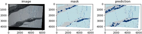
A kernel part of the feature extraction is a DL-based classification algorithm, which is extremely time consuming and hampers the on-demand analyses of sea ice analyses. The algorithm involves high computational intensity. The data required for this task would be substantial, including high-resolution images, as well as additional geospatial and environmental data to aid in classification, which also involves high data intensity. In addition, the DL-based classification algorithm also requires a significant amount of labelled training data to optimize its performance, which also involves substantial data dependency. Overall, this application involves a complex and resource-intensive workflow that requires management of both computational and data resources. The incorporation of GPU enablement would significantly speed up the process and enable on-demand analyses.

Tweet classification: The COVID-19 pandemic impacted the entire world disastrously. Millions of tweets were posted every day. It is important to understand public sentiment and attention from a spatiotemporal perspective but categorizing all social media contents for research will be very time-consuming. Therefore, this application categorizes COVID-19 related tweets into 7 categories (prevention, transmission, politics, economy, emotion, symptoms, treatment) by using a CNN model. We analysed tweets from January to August 2020 to mine the categories of COVID-19 related tweets and discover what aspects publics cared about COVID-19 in different spatiotemporal scales. This open-source package was later utilized to discover the spatiotemporal patterns of public opinions on COVID-19 vaccines from October 1st, 2020, to May 21st, 2021, as shown in Figure 2 (Wang et al. 2022).

Figure 2. Spatial distribution of Public Engagement Score (PES) in the United States from October 1st, 2020, to May 21st, 2021.

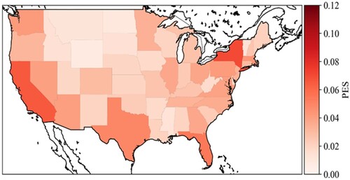
This application contains a small-size training dataset, which only includes around 800 tweets with their corresponding labels. The training process only requires low computational intensity and data intensity. The accuracy of the model and the usefulness of the categorized tweets are dependent on the quality and amount of data used to train and test the model, but this model can train tweet datasets with several types of labels which only requires a moderate data dependency.

Cloud classification: Precipitation is one of the most significant contributing factors to destructive natural disasters globally including hurricanes, floods, and droughts. Convective precipitation with abnormal activities of convective systems may lead to severe urban floods, landslides, and flash floods. To detect rainy and convective clouds with high efficiency, this application developed a DNN method to classify rainy and non-rainy clouds based on Brightness Temperature Differences (BTDs) and Reflectance (Ref) derived from Advanced Baseline Imager (ABI). Convective and stratiform rain clouds are also separated using similar spectral parameters expressing the characteristics of cloud properties. The precipitation events used for training and validation are obtained from the Integrated Multi-satellite Retrievals for GPM (IMERG) V05B data, which covered the south-eastern coast of the U.S. during the 2018 rainy season. This automatic cloud classification system could be deployed for extreme rainfall event detection, real-time forecasting, and decision-making support in rainfall-related disasters (Liu et al. 2019; Figure 3).

Figure 3. Cloud classification categorizes the cloud into various classes to identify the rainy cloud for disaster response.

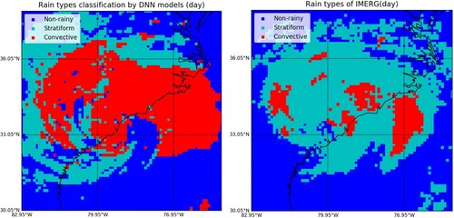
DNN models are computationally intensive due to their large number of parameters and the need for extensive training on large datasets. Additionally, this application involves analyzing data from the ABI and the IMERG V05B dataset. These datasets contain substantial amounts of satellite imagery data, and the accuracy of the results are highly dependent on the quality and amount of data analyzed, but different cloud data can be selected as training datasets. Therefore, this model requires high data intensity but moderate dependency.

PM2.5 Retrieval: Particulate Matter (PM) consists of a complex mixture of solid and liquid particles of organic and inorganic substances suspended in the air. As a common proxy indicator for air pollution, PM2.5 is extremely hazardous to human health as it can be easily inhaled into the human chest and enter the respiratory system, (Song et al. 2019) and causes millions premature deaths annually around the world. This application aims to develop an innovative methodology to retrieve the PM2.5 over global scale and further downscale the spatiotemporal resolution to 1 km and hourly level in some key regions using AI/DL methods (Figure 4). The results generate a high spatiotemporal resolution to provide data basis for public health decision making and air quality pattern analytics.

Figure 4. PM2.5 values are retrieved from GOES-16/17 and MERRA-2 data based on ground observations and AI/ML models/algorithms.

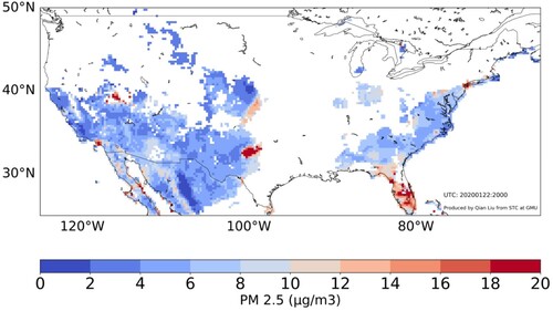
This application requires complex calculations and significant computing resources, as it involves processing and analysing vast amounts of data to generate high-resolution outputs. The accuracy of the PM2.5 estimates is affected by the quality and coverage of satellite observations, as well as the availability and accuracy of ground-based measurements used for validation. Therefore, this application also involves high computational intensity, high data intensity, and high data dependency.

Satellite2Map: Theme maps have become increasingly common in the technological era, but creating map is expensive and time consuming (Kamil and Shaikh 2019). The simplicity of theme maps allows them to be a key feature of various mapping applications. This application uses Conditional Generative Adversarial Network (GAN) to automatically convert Earth Observation (EO) imagery into a real map through identifying features on images, such as water, roads, buildings, plant life, and other features as shown in Figure 5 (Ganguli, Garzon, and Glaser 2019). The Earth observation data is downloaded from Google Earth and latent space vectors are extracted from satellite image. Latent space vectors are compressed depictions of the satellite images, and they are inputted into the GAN model to create new maps.

Figure 5. Satellite2Map generates a theme map based on Earth observation data (Ganguli, Garzon, and Glaser 2019).

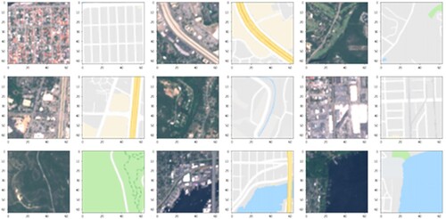
This application is also computationally intensive and data-intensive because GAN consists of two neural networks competing against each other, with one trying to generate realistic data (in this case, a map) and the other trying to distinguish between real and generated data. a large amount of Earth Observation (EO) imagery is required for training the GAN model. In addition, the accuracy of the generated maps also depends on the quality and quantity of the input data, but any pairs of Earth observation data and latent space vectors can be selected as training dataset. Therefore, this application only requires a moderate data dependency.

3.2 Platform introduction

We engaged 5 different types of platforms in the study from the most popular (PC) to specialized (GPU cluster). Their specific configurations are introduced in the Table 2.

(1)	Windows desktop with a NVIDIA GeForce RTX 3070 GPU

Table 2. Hardware configuration of each computing platform.

Hardware\platform	Desktop	Google Colab	AWS	NASA supermicro	Microsoft
CPU (Core #: Speed Ghz)	8 cores Intel(R) Core (TM) i7-10700 K CPU @ 3.80 GHz 3.79 GHz	2 vCPUs Xeon Processor (2.2 GHz)	48 vCPUs, Intel Xeon Scalable (Cascade Lake), ∼3.2 GHz	NVLink Dual Intel Xeon Cascade Lake Gold 6248 CPUs, 20 cores each (2.50 GHz)	Intel(R) Xeon(R) CPU E5-2690 v4 @ 2.60 GHz 6 cores
GPU (Core #, Speed Ghz, Memory size)	1x NVIDIA GeForce RTX 3070 with 8 GB of VRAM	1x NVIDIA Tesla T4 GPU with 16 GB of VRAM	4x NVIDIA Tesla T4 GPUs with 16 GB of VRAM	4x NVIDIA V100 GPUs with 32 GB of VRAM	1x GV100GL [Tesla V100 PCIe 16GB]
RAM size	32.0 GB	12.6 GB	192 GB	768 GB	112 GB
Storage	SN730 NVMe WDC 256G	33 GB on Google Drive	900 GB NVMe storage	3.8 TB of RAID protected NVMe drives	SCSI virtual Disk 1TB

The windows desktop is used for benchmarking and serves as an initial reference. All applications were originally designed and programmed on this computer. All other platforms have the same running environment configuration as this desktop, such as Python and Python package version. This platform is suitable for individual researchers who work on small to medium-sized datasets and can perform their computations locally on their desktop. However, the accessibility of this platform is limited to the researcher's research resource, and it may not be suitable for large-scale computations or collaborations with other researchers.

(2)	AWS G4dn instances

AWS provides G4dn instances that are optimized for graphics-intensive workloads, such as 3D rendering, video encoding, and machine learning. They provide cloud-based computing resources with high-performance GPUs, making it an attractive option for domain scientists who need to process large amounts of data. The Tesla T4 GPUs are optimized for DL workloads and provide fast training times. The cloud-based nature of this platform makes it accessible from anywhere with an Internet connection, and it also allows for scalability as researchers can increase or decrease resources as needed.

(3)	Google Colab

Google Colab is a free online platform that allows users to run and execute code in a variety of programming languages, including Python, R, and Julia. It is a cloud-based platform that provides free access to GPUs and CPUs for research and education purposes. It is a suitable option for researchers who have limited resources or are new to DL and need to experiment with small to medium-sized datasets. The platform is easily accessible, and users can collaborate and share their work with others.

(4)	Microsoft Azure

Microsoft Azure provides cloud-based computing resources with a range of GPU options suitable for different workloads, including ML and DL. The platform offers scalability and can handle large-scale computations, making it an attractive option for domain scientists who need to process substantial amounts of data. It also provides collaboration and sharing features, making it easy for researchers to work together.

(5)	NASA Supermicro

NASA Supermicro provides high-performance computing resources for scientific research, including ML and DL. The platform is designed to handle large-scale computations and is suitable for domain scientists who need to process large datasets or run complex simulations. However, the platform cannot be easily accessible to individual researchers due to security restrictions, and it requires specialized knowledge to use effectively. This project has applied and was approved for using NASA supermicro to test the performance of all 5 applications.

3.3 Model parallel training strategies

Two common approaches have been developed to support model parallel training, including data parallelism (Krizhevsky 2014) and model parallelism (Dean et al. 2012). In the data parallelism approach, the same model is distributed to multiple GPUs and each GPU is responsible for training the model on a different subset of data (Krizhevsky 2014). In model parallelism, a model is split into several parts which are then sent to multiple GPUs to train separately (Dean et al. 2012). These strategies allow the model to be trained in parallel, making it possible to significantly reduce the time required to train larger and more accurate models.

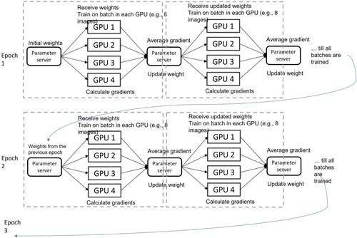
Data parallelism is the most common model parallel training strategy. It is suitable for computationally intensive layers with a relatively small number of parameters. As shown in Figure 6, the data parallelism approach typically runs iteratively with the following initial weights and updates: (1) dataset is divided into smaller chunks and each chunk is assigned to a different GPU. Each GPU has a completed model and assigned data chunks; (2) a parameter server initializes model weights and sends weights to multiple GPUs; (3) every GPU trains the model on its assigned chunk of data and calculates the gradient; (4) GPUs send the computed gradient to the parameter server; (5) the parameter server produces a single and updated model based on gradients collected from all GPUs; (6) the parameter server sends the updated model weights to all GPU devices; (7) the above steps are repeated until the model has converged. Data parallelism strategy benefits distributed GPU computing by significantly reducing train time as the model could be trained in parallel on multiple GPUs. It also enables high scalability since the data parallelism strategy could be deployed on a large number of GPUs by simply dividing data into small chunks. Noticeably, data parallelism is relatively easy to implement since it did not require significant changes to the model or the training process.

Figure 6. An example workflow of the data parallel training approach with iterative weights and updates.

Model parallelism is suitable for layers with a large number of parameters (e.g. fully connected layer). Compared to data parallel training, it is more complicated. Model parallelism strategy typically involves steps as follows: (1) divide the model into several layers or blocks of layers that can be trained in different GPUs; (2) assign model blocks to multiple GPUs; (3) divide training data into batches and assign each batch to a specific GPU; (4) model block on each GPU are trained with assigned training data and then gradients and model parameters are synchronized among GPUs at each training step; (5) the gradients from all GPUs are aggregated to update model parameters; (6) the above steps are repeated until the model has converged. Noticeability, although model parallelism strategy makes it possible to train larger and more accurate models in a shorter amount of time, it can be complex to implement the strategy since the original model needs to split into different parts and model parameters, and gradient should be synchronized among multiple GPUs.

We will only focus on adopting data parallelism strategy to support distributed training DL-based Earth science applications in this study. We will optimize the open-source applications to support model parallelism in future studies.

4. Experiment design and performance evaluation

4.1 Experiment setup and design

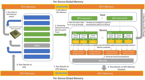
We compared applications with different AI/ML algorithms that run on CPU, GPU, and multi-GPU. The workflow including package installation, model preparation, cluster enablement, testing and validation is illustrated in Figure 7. When an application runs on CPU, all data and model are processed by CPU. When an application runs on GPU, Sequential CPU code and data will pass to CPU to process, GPU code will pass to GPU to process, then CPU will pass the data to CPU Memory then to GPU Memory. Once the GPU receives the code, the GPU kernel will be launched to pass the same piece of code to different threads and process all data passed from GPU memory. CUDA API will invoke multithreaded streaming multiprocessors in GPU to generate the results and eventually the results will be passed from GPU memory to CPU memory then to CPU (Figure 8).

Figure 7. The workflow of testbed process including analysis, package installation, model preparation, cluster enablement, testing and validation.

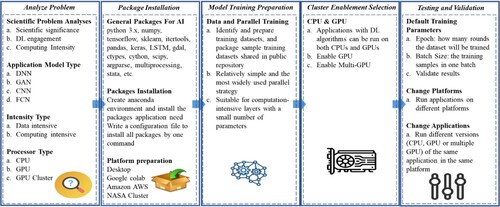
Figure 8. The dataflow between GPU and CPU in a GPU-based DL application.

Each application was tested with and without GPU enabled on a Desktop. Each application was also tested with single-GPU and multi-GPU (4 GPUs) on NASA Supermicro, AWS G4dn, and Microsoft Azure. Google Colab only provided an environment with single GPU. The total running time of each application was recorded.

4.2 Experiment results

4.2.1 Runtime performance

The following table shows the running time of each application with different types of processors. The NASA platform on Multiple GPU has the shortest runtime of 46 m on the cloud classification application, whereas the desktop platform on CPU has the longest run time of 3 h 29 m on the application. The PM2.5 application on the Google Colab single GPU has the lowest runtime of 7 m while the NASA GPU has the highest runtime of 24 m. NASA single GPU recorded the lowest runtime of 2 h 44 m on the ArcCI application while the desktop CPU recorded the maximum runtime of 94 h 37 m on the ArcCI application. The AWS platform on the single GPU has the shortest runtime of 7s for the Tweets Classification application while the Microsoft Single GPU has the highest runtime of 45s. The NASA multi-GPU has the lowest runtime of 2 h 38s for the Satellite2map application while the desktop CPU has the highest runtime of 70 h 21 m for the Satellite2map. Table 3 shows the details for runtime of five applications in different platforms, and Figure 9 shows the percentage for runtime of five applications in different platforms by comparing to the runtime on desktop CPU (assuming the runtime on desktop is 100%).

Figure 9. The runtime comparison of five applications in percentage among different platforms by comparing to the runtime on desktop CPU (assuming the runtime for each application on desktop is 100%).

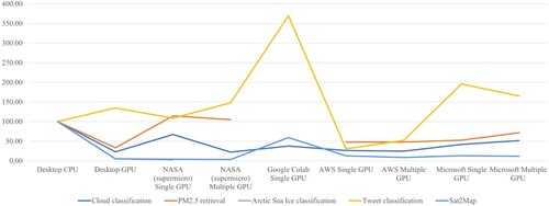
Table 3. Average runtime of the five applications and standard deviations (SD) of runtime for 5 iterations in different platforms with varying CPU and GPU usages.

	Desktop		NASA Supermicro		Google Colab	AWS G4dn instance		Microsoft Azure
	CPU/SD	GPU/SD	Single GPU/SD	Multiple GPU/SD	Single GPU/SD	Single GPU/SD	Multiple GPU/SD	Single GPU/SD	Multiple GPU/SD
Cloud classification	3h29 m/ 0.03	48 m/0.02	140 m/ 0.04	46 m/ 0.03	79 m/ 0.03	55 m / 0.02	51 m/ 0.01	87 m/ 0.01	108 m/ 0.02
PM2.5 retrieval	21 m/ 0.02	7 m/0.01	24 m/0.02	22 m/0.02	2 m/0.01	9m30s/0.01	10 m/0.01	11 m/0.01	15 m/0.01
Arctic Sea Ice classification	94h22 m/0.80	4h25 m(1)/0.04	2h44 m/0.05	N/A(2)	N/A	9h36m/0.96	N/A(2)	3h2 m/0.03	N/A
Tweet classification	23s/0.44	31s/0.54	25s/1.41	34s/2.68	1m25s/2.54	7s/2.32	12s/1.87	45s/3.67	38s/1.30
Sat2Map	70h21 m/0.39	3h34 m/0.05	3 h/0.04	2h23 m/0.05	>7 h (3)	8 h/0.11	6h4 m/0.13	7h17 m/0.17	8h12 m/0.16

Note: 1. when the ArcCI application was run in desktop using GPU mode, batch size was changed to 10 from 60, otherwise, the GPU would be out of memory. The batch size was set to 60 when the application was run on NASA Supermicro.

2. The ArcCI application cannot be run with multiple GPU mode since the DL package it utilizes cannot successfully support multiple GPUs.

3. The sat2map runtime in google Colab records runtime about 168 epochs and other experiments set epochs to 1000. We cannot have the exact time on Google Colab due to session timeout so we cannot find the standard deviation.

4. NAN values were removed in the Google Colab platform due to an error caused by null values, thus the size of the train dataset is different from that on other platforms.

5. The Standard deviation for tweet classifications is based on seconds, and rest of four applications are based on hours. For standard deviation lower than 0.01 we count as 0.01.

4.2.2 Single-GPU experiment results correlation analysis

Correlation analysis is conducted to produce a correlation coefficient r as shown in the equation (1(1) $\mathrm{r}={\displaystyle \frac{\sum [(\mathrm{runtim}{\mathrm{e}}_{\mathrm{i}}-\overline{\mathrm{runtime}})({\mathrm{x}}_{\mathrm{i}}-\overline{\mathrm{x}})]}{\surd \sum {(\mathrm{runtim}{\mathrm{e}}_{\mathrm{i}}-\overline{\mathrm{runtime}})}^2\sum {({\mathrm{x}}_{\mathrm{i}}-\overline{\mathrm{x}})}^2}}$(1) ) where x represents hardware configurations in a computing environment. The coefficient r is a numerical value that ranges between −1 and 1. −1 indicates a perfect negative correlation between the variables, while 1 indicates a perfect positive correlation and 0 indicates no correlation between the variables. In this study, a correlation analysis was done between the configurations of single GPU VMs and the runtime of each application to understand the relationship between VM configurations and runtime performance. (1) $\mathrm{r}={\displaystyle \frac{\sum [(\mathrm{runtim}{\mathrm{e}}_{\mathrm{i}}-\overline{\mathrm{runtime}})({\mathrm{x}}_{\mathrm{i}}-\overline{\mathrm{x}})]}{\surd \sum {(\mathrm{runtim}{\mathrm{e}}_{\mathrm{i}}-\overline{\mathrm{runtime}})}^2\sum {({\mathrm{x}}_{\mathrm{i}}-\overline{\mathrm{x}})}^2}}$(1) Table 4 shows the correlation between each application and configuration elements based on experiment results. In general, the runtime is negatively related to the CPU speed for single-GPU applications. The faster the CPU speed, the less runtime the application will take. The GPU core and memory are not fully utilized since the applications are single-GPU bases, thus the correlation between runtime and GPU memory/core are positive for some applications. It indicates that improving the number of GPUs cannot guarantee runtime performance improvement for DL applications without parallelism strategy.

Table 4. Correlation between runtime and VM configuration for the five single-GPU based applications.

	Cloud	PM2.5	ArcCI	Sat2Map	Tweets
CPU Core	−0.13652	0.266838	0.896987	0.273313	−0.48629
CPU Speed	−0.66137	−0.14398	−0.0781	−0.25496	0.213986
GPU Memory	0.942456	0.845117	−0.00328	−0.33031	−0.56639
GPU core	0.392476	0.674978	0.570109	−0.09861	−0.34954
Storage & Motherboard speed	−0.32522	−0.04566	0.663085	0.633881	−0.11338
Ram Size	0.857276	0.95662	−0.10479	−0.54898	0.345172

4.2.3 Multiple-GPU experiment results correlation analysis

Similar correlation analysis was done for the five multiple-GPU based applications and VM configuration as shown in Table 5. The analytical results show that the CPU speed also plays a significant role for multiple-GPU applications. The correlation between GPU core and runtime are positive for all applications as expected.

Table 5. Correlation between runtime and VM configuration for the five multiple-GPU based applications.

	Cloud	PM2.5	ArcCI	Sat2Map	Tweets
CPU Core	−0.70642	−0.57924	–	−0.04515	0.984778
CPU Speed	−0.31314	−0.88371	–	−0.48913	−0.95789
GPU Memory	−0.56154	0.909935	–	0.989512	0.356689
GPU core	−0.99736	0.674978	–	0.619854	−0.63063
Storage & Motherboard speed	0.642519	−0.86321	–	−0.99906	0.250144
Ram Size	−0.6505	0.857879	–	0.999457	−0.26026

4.2.4 Optimization

TensorFlow Profiler (Figure 10), part of TensorFlow’s visualization toolkit, is used to quantify the running time of each application and identify the performance bottleneck in each step. Target metrics gathered include kernel launch time and device compute time as part of a high-level summary of model performance across step-time. Each runtime experiment is conducted in a similar manner. The times at which the model begins and finishes training is logged as well as information on the compute node used and performance metrics gathered using TensorFlow profiler. Additional metrics including model accuracy are also logged for comparison to scientifically published results.

Figure 10. TF Profiler step-time results in milliseconds for Cloud Classification without XLA Compiler.

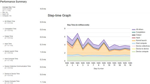
From the TensorFlow profiler, we discovered the total running time was majorly spent on the kernel launch time and device compute time. To reduce the kernel launch time and device compute time, XLA compiler was utilized. XLA (Accelerated Linear Algebra) is a domain-specific compiler for linear algebra that can accelerate TensorFlow models. It compiles the TensorFlow graph into a sequence of computation kernels generated specifically for the given model (Tensorflow 2022). Since these kernels are unique to the model, they can exploit model-specific information for optimization. When a model is trained regularly, the graph launches three kernels for three different functionalities: multiplication, addition, and reduction (Tensorflow 2022). However, XLA can optimize the graph so that it computes the result in a single kernel launch. It does this by ‘fusing’ the addition, multiplication, and reduction into a single GPU kernel, so that it also reduces the compute time for each GPU (Tensorflow 2022).

Using cloud classification as an example, as the results showing in Figures 10 and 11, with implementation of XLA compiler, the kernel launch time is reduced from 1.9 ms to 1.0 ms. The Device Compute Time is reduced from 1.1 ms to 0.2 ms. It greatly optimized computing performance in each step of the training process, meanwhile the model accuracy only changed 1% as shown in the Table 6.

Figure 11. Cloud Classification Performance results for each step in milliseconds with XLA Compiler.

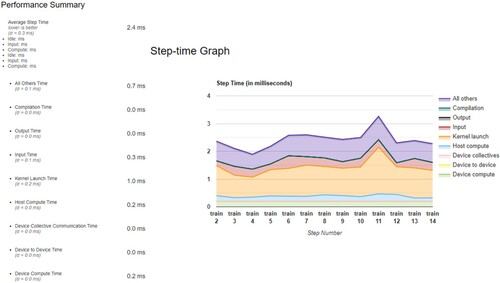
Table 6. Cloud Classification performance comparison with and without implementation of XLA compiler.

	Total Time in each step	Kernel Launch Time	Device compute time	Total Time for the whole application	Model accuracy
Without XLA	4.6ms	1.9ms	1.1ms	48 m	0.8612
With XLA	2.4ms	1.0ms	0.2ms	29m	0.8565

4.3. Discussion

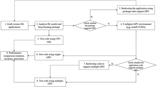
To migrate Earth science AI/ML application onto GPU Platform and compare performance among CPU, single-GPU, and multi-GPU, we conclude a step list that researchers need to go through. Table 7 shows what steps each application in this study had taken.

1. Analyze DL model and DL package used by the application: before migrating an Earth science DL application to GPU, researchers need to analyze the DL model and the DL package used by the application. They should check if the package has GPU support, the DL model complexity, the size of the dataset, and the computational requirements. This analysis helps to determine if the application will benefit from GPU acceleration.

2. Check whether the package supports GPU: Researchers need to check if the DL package used by the application supports GPU acceleration. Many DL packages such as TensorFlow, PyTorch, and Keras provide GPU support. Researchers should also ensure that the GPU driver is compatible with the DL package.

3. Redevelop the application using packages that support GPU: If the DL package used by the application does not support GPU acceleration, researchers should consider redeveloping the application using packages that support GPU acceleration. This may require additional time and resources, but it can significantly improve runtime performance.

4. Configure GPU environment library based on DL package version: Researchers need to configure the GPU environment library based on the DL package version used by the application. The GPU environment library includes CUDA and CUDNN, and their versions should be compatible with the DL package and Python version used by the application.

5. Check whether the application code supports multiple GPU: Researchers should check if the application code supports multiple GPUs. If the application code does not support multiple GPUs, it may require modification to partition and distribute the data and models on multi-GPU.

6. Redevelop code to support multiple-GPU by partitioning and distributing the data and models on multi-GPU: If the application code does not support multiple GPUs, researchers need to redevelop the code to partition and distribute the data and models on multi-GPU. This can significantly improve runtime performance.

7. Install performance monitoring tools to collect host activities and GPU traces: Researchers should install performance monitoring tools such TF-Profiler for Tensorflow to collect host activities and GPU traces. These tools help identify bottlenecks and performance issues during GPU acceleration.

8. Performance comparison (runtime, accuracy, precision): Researchers should conduct a performance comparison among the original CPU-based application, the single-GPU-accelerated application, and the multi-GPU-accelerated application. The comparison should include runtime, accuracy, and precision.

9. Optimize the performance based on detected bottleneck from performance monitoring tools: Researchers need to optimize the performance of the GPU-accelerated application based on the detected bottleneck from the performance monitoring tools. This may require further code optimization, data preprocessing, or tuning of hyperparameters. The goal is to achieve the best possible runtime performance without compromising accuracy and precision.

Table 7. Steps for each application to be migrated onto GPU Platform and to compare their performance among CPU, single-GPU, and multi-GPU.

	A	B	C	D	E	F	G	H	I
ArcCI	X	X	X	X			X	X	X
Tweet classification	X	X	X	X	X	X	X	X	X
Cloud classification	X	X	X	X	X	X	X	X	X
PM2.5 Retrieval	X	X	X	X	X	X	X	X	X
Satellite2Map	X	X	X	X	X	X	X	X	X

In this study, five different Earth science applications with different parameter inputs and DL algorithms were run on different platforms in CPU, single-GPU, and multi-GPU modes. The runtime of the same application varies on these platforms with different machine configurations. In general, the runtime of experiments running on CPU is longer than that of experiments running on GPU except for the tweet classification application, the input data size of which is very small. The total runtime of the tweet classification application is less than half a minute on a desktop using the CPU model, and from the experiment results, we can find that it is hard to improve runtime performance with GPU when the input data size and computation is very small since the computational time is smaller compared to the time of data transmission.

By comparing the runtime of experiments on the same platform running with single-GPU and multiple-GPU, the decrease in the runtime is not as significant as expected for most applications. One plausible reason is that an application may cost extra time when the whole program synchronizes the data and model among GPUs and CPU (Sun et al. 2019). Based on the experiment results, we found that the decrease in the runtime is not linearly related to the increment of GPU numbers, especially for applications with relatively small input data sizes.

In addition, we implemented a simple and direct data-parallel strategy to run these applications with the support of multiple-GPU on different platforms. However, the percentage of GPU usage varies across platforms even with the same code. Taking cloud classification as an example, the percentage of GPU usage is quite different on different platforms. When the application was run on AWS and Azure with 4 GPUs, the utilization percentage of each GPU was around 20% on the AWS platform. However, the percentage was 0% for each GPU on the Azure platform. The difference in GPU utilization needs further investigation between application developers and platform providers since different platforms demonstrate different results to identify the reason and potential improvements. However, the results of the experiments indicate that each GPU may not be able to be fully utilized with the built-in parallel strategy.

For a given Earth science DL application, researchers could follow the workflow (Figure 12) to enable the application to support single-GPU or multiple-GPU to improve runtime performance. However, to optimize the runtime performance of these applications, it is crucial to enable support for single-GPU or multiple-GPU. Specifically, we recommend giving special attention to applications initially designed for CPUs, as their code often requires modification to be compatible with GPUs. Moreover, even applications originally designed for single GPU must be parallelized to work on multi-GPU. It is worth noting that increasing the number of GPUs does not necessarily guarantee faster running times, highlighting the importance of proper parallelization strategies.

Figure 12. Recommendation workflow of utilizing GPU to support Earth science applications.

Additionally, it should be noted that different GPUs require specific GPU drivers, such as CUDA, and driver libraries, such as CUDNN. It is essential to ensure that each driver and library version is compatible with the corresponding Python version and package version. For example, the required versions of CUDA, CUDNN, Python, and TensorFlow for this project are CUDA 11.0, CUDNN 8.0, Python 3.8.12, and TensorFlow 2.4.1, respectively. Any mismatches between these versions may result in the failure of running applications.

For the next steps of this study, we will study how to optimize the performance of GPU and multi-GPU based on these five existing applications such as reducing the synchronization time of data and model among CPUs and GPUs. In addition, considering GPU utilization with the same code varied in different platforms, investigating the reason causes different GPU utilizations and optimizing the GPU utilization across different platforms will also be conducted.

5. Conclusion

In this study, we highlighted five existing sample Earth science AI applications, revised the DL-based models/algorithms to support GPU parallel training, delivered application source code and tutorials, and tested performance of common computing platforms (e.g. Amazon AWS, Google Colab and Microsoft Azure) about the support to the applications. Application software packages, performance comparisons across different platforms, along with performance results. This study provides a better understanding of how various AI/ML Earth science applications can be supported by GPU computing and could help researchers in the Earth science domain better adopt GPU computing for their AI/ML research. Relevant software package and user guide have been made publicly available in GitHub.

We found that GPU should be considered to run Earth science DL applications, because generally, adopting GPU can reduce the running time. However, if the input data size of a DL application is small, we would suggest using single-GPU to reduce the cost. It is hard to improve runtime performance with multi-GPU when the input data size is very small, especially when the computational time is smaller compared to the time of data transmission. In addition, utilizing multiple GPU and data-parallel strategies does not guarantee a speed-up, because DL algorithms vary for different applications. Lastly, we suggest paying more attention to applications initially designed for CPUs that will require extra efforts, such as adding extra or even replacing existing programming packages. Applications originally designed for single GPU also need parallelization to make them work on multi-GPU, meanwhile, more GPUs do not necessarily mean faster running time.

In the future, more experiments could be conducted to optimize the utilization of GPU to support parallel training in Earth Science AI applications. The impact factors and bottlenecks of CPU, GPU, and multi-GPU utilization need more investigation to best utilize GPU in Earth AI research. Additional Earth science applications that utilize different types of AI models such as graph neural networks and recurrent neural networks could be added to the testbed to cover the most advanced DL models.

Acknowledgements

NASA Center for Climate Simulations provided partial GPU resources for the test. The applications were developed by various researchers. IBM, Mircosoft, AWS, and Google for collaborated with us on GPU environment configuration. We thank the anonymous reviewers for their valuable comments.

Disclosure statement

No potential conflict of interest was reported by the author(s).

Additional information

Funding

This work is financially supported by NSF I/UCRC (1841520), NASA Goddard CISTO, and NASA AIST programs.

References

- Bhowmik, Moumita, Manmeet Singh, Suryachandra Rao, and Souvik Paul. 2022. “DeepClouds. ai: Deep learning enabled computationally cheap direct numerical simulations.” arXiv preprint arXiv:2208.08956.
- Caraballo-Vega, Jordan, Mark Carroll, Jian Li, and Daniel Duffy. 2021. “Towards Scalable and GPU Accelerated Earth Science Imagery Processing: An AI/ML Case Study.” AGU Fall Meeting Abstracts 2021: N21A–28.
- Chao, Fang, Yang Chongjun, Chen Zhuo, Yao Xiaojing, and Guo Hantao. 2011. “Parallel Algorithm for Viewshed Analysis on a Modern GPU.” International Journal of Digital Earth 4 (6): 471–486. https://doi.org/10.1080/17538947.2011.555565.
- Che, Shuai, Michael Boyer, Jiayuan Meng, David Tarjan, Jeremy W. Sheaffer, and Kevin Skadron. 2008. “A Performance Study of General-Purpose Applications on Graphics Processors Using CUDA.” Journal of Parallel and Distributed Computing 68 (10): 1370–1380. https://doi.org/10.1016/j.jpdc.2008.05.014.
- Chen, Ying, Xu Ouyang, and Gady Agam. 2019. “ChangeNet.” In Proceedings of the 3rd ACM SIGSPATIAL International Workshop on AI for Geographic Knowledge Discovery, 24–31. https://doi.org/10.1145/3356471.3365232
- Dean, Jeffrey, Greg S. Corrado, Rajat Monga, Kai Chen, Matthieu Devin, Quoc V. Le, Mark Z. Mao, et al. 2012. “Large Scale Distributed Deep Networks.” Advances in Neural Information Processing Systems 25.
- Feng, XueShang, DingKun Zhong, ChangQing Xiang, and Yao Zhang. 2013. “GPU-accelerated Computing of Three-Dimensional Solar Wind Background.” Science China Earth Sciences 56 (11): 1864–1880. https://doi.org/10.1007/s11430-013-4661-y.
- Fu, Cong, Zhenhua Wang, and Yanlong Zhai. 2017. “A CPU-GPU Data Transfer Optimization Approach Based on Code Migration and Merging.”In 16th International Symposium on Distributed Computing and Applications to Business, Engineering and Science (DCABES), 23–26.
- Ganguli, Swetava, Pedro Garzon, and Noa Glaser. 2019. “GeoGAN: A conditional GAN with reconstruction and style loss to generate standard layer of maps from satellite images.” arXiv preprint arXiv:1902.05611.
- Gao, Jianwei, Yi Sun, Bing Zhang, Zhengchao Chen, Lianru Gao, and Wenjuan Zhang. 2019. “Multi-GPU Based Parallel Design of the ant Colony Optimization Algorithm for Endmember Extraction from Hyperspectral Images.” Sensors 19 (3): 598. https://doi.org/10.3390/s19030598.
- Gregg, Chris, and Kim Hazelwood. 2011. “Where is the Data? Why you Cannot Debate CPU vs. GPU Performance Without the Answer.” (IEEE ISPASS) IEEE International Symposium on Performance Analysis of Systems and Software, 134–144. https://doi.org/10.1109/ISPASS.2011.5762730.
- Ikram, Ben Abdel Ouahab, Boudhir Anouar Abdelhakim, Astito Abdelali, Bassam Zafar, and Bouhorma Mohammed. 2019. “Deep Learning Architecture for Temperature Forecasting in an IoT LoRa Based System.” In Proceedings of the 2nd International Conference on Networking, Information Systems & Security, 1–6.
- Janowicz, Krzysztof, Song Gao, Grant McKenzie, Yingjie Hu, and Budhendra Bhaduri. 2020. “GeoAI: Spatially Explicit Artificial Intelligence Techniques for Geographic Knowledge Discovery and Beyond.” International Journal of Geographical Information Science 34 (4): 625–636. https://doi.org/10.1080/13658816.2019.1684500.
- Kamath, Harsh G., Manmeet Singh, Lori A. Magruder, Zong-Liang Yang, and Dev Niyogi. 2022. “GLOBUS: GLObal Building heights for Urban Studies.” arXiv:2205.12224.
- Kamil, Anwar, and Talal Shaikh. 2019. “Literature Review of Generative Models for Image-to-Image Translation Problems.” In 2019 International Conference on Computational Intelligence and Knowledge Economy (ICCIKE), 340–345. IEEE.
- Krizhevsky, Alex. 2014. “One weird trick for parallelizing convolutional neural networks.” arXiv preprint arXiv:1404.5997.
- Li, Wenwen, and Chia-Yu Hsu. 2022. “GeoAI for Large-Scale Image Analysis and Machine Vision: Recent Progress of Artificial Intelligence in Geography.” ISPRS International Journal of Geo-Information 11 (7): 385. https://doi.org/10.3390/ijgi11070385.
- Li, Yun, Ruixin Yang, Chaowei Yang, Manzhu Yu, Fei Hu, and Yongyao Jiang. 2017. “Leveraging LSTM for Rapid Intensifications Prediction of Tropical Cyclones.” ISPRS Annals of Photogrammetry, Remote Sensing & Spatial Information Sciences 4: 101–105.
- Li, Yun, Manzhu Yu, Mengchao Xu, Jingchao Yang, Dexuan Sha, Qian Liu, and Chaowei Yang. 2020. “Big Data and Cloud Computing.” Manual of Digital Earth, 325–355.
- Liu, Qian, Yun Li, Manzhu Yu, Long S Chiu, Xianjun Hao, Daniel Q Duffy, and Chaowei Yang. 2019. “Daytime rainy cloud detection and convective precipitation delineation based on a deep neural Network method using GOES-16 ABI images.” Remote Sensing 11 (21).
- McKiernan, Erin C., Philip E. Bourne, C. Titus Brown, Stuart Buck, Amye Kenall, Jennifer Lin, Damon McDougall, et al. 2016. “How open science helps researchers succeed.” eLife 5.
- NASA Science “Open-Source Science Initiative / Science Mission Directorate,” 2023. https://science.nasa.gov/open-science-overview.
- Oeser, Jens, Hans-Peter Bunge, and Marcus Mohr. 2006. International conference on high performance computing and communications, 31–40. Springer.
- Okamoto, Taro, Hiroshi Takenaka, Takeshi Nakamura, and Takayuki Aoki. 2010. “Accelerating Large-Scale Simulation of Seismic Wave Propagation by Multi-GPUs and Three-Dimensional Domain Decomposition.” Earth, Planets and Space 62 (12): 939–942. https://doi.org/10.5047/eps.2010.11.009.
- Reichstein, Markus, Gustau Camps-Valls, Bjorn Stevens, Martin Jung, Joachim Denzler, Nuno Carvalhais, and Prabhat. 2019. “Deep Learning and Process Understanding for Data-Driven Earth System Science.” Nature 566 (7743): 195–204. https://doi.org/10.1038/s41586-019-0912-1.
- Ryoo, Shane, Christopher I. Rodrigues, Sara S. Baghsorkhi, Sam S. Stone, David B. Kirk, and Wen-mei W. Hwu. 2008. “Optimization Principles and Application Performance Evaluation of a Multithreaded GPU Using CUDA.” 13th ACM SIG-PLAN Symposium on Principles and Practice of Parallel Programming, 73–82.
- Schultz, Martin G., Clara Betancourt, Bing Gong, Felix Kleinert, Michael Langguth, Lukas Hubert Leufen, Amirpasha Mozaffari, and Scarlet Stadtler. 2021. “Can Deep Learning Beat Numerical Weather Prediction?.” Philosophical Transactions of the Royal Society A: Mathematical, Physical and Engineering Sciences 379 (2194): 20200097. https://doi.org/10.1098/rsta.2020.0097.
- Sekhar Biswas, Mriganka, and Manmeet Singh. 2022. “Trustworthy modelling of atmospheric formaldehyde powered by deep learning.” arXiv e-prints: arXiv-2209.
- Sha, Dexuan, Xin Miao, Mengchao Xu, Chaowei Yang, Hongjie Xie, Alberto M Mestas-Nuñez, Yun Li, Qian Liu, and Jingchao Yang. 2020. An on-demand service for managing and analyzing arctic sea ice high spatial resolution imagery 5.
- Singh, Manmeet, Nachiketa Acharya, Suryachandra A. Rao, Bipin Kumar, Zong-Liang Yang, and Dev Niyogi. 2022. “Short-range forecasts of global precipitation using deep learning-augmented numerical weather prediction.” arXiv preprint arXiv:2206.11669.
- Song, Yimeng, Bo Huang, Qingqing He, Bin Chen, Jing Wei, and Rashed Mahmood. 2019. “Dynamic assessment of PM2. 5 exposure and health risk using remote sensing and geo-spatial big data.” Environmental Pollution 253: 288–296.
- Subramaniam, Shankar, Naveenkumar Raju, Abbas Ganesan, Nithyaprakash Rajavel, Maheswari Chenniappan, Chander Prakash, Alokesh Pramanik, Animesh Kumar Basak, and Saurav Dixit. 2022. “Artificial Intelligence Technologies for Forecasting Air Pollution and Human Health: A Narrative Review.” Sustainability 14 (16): 9951. https://doi.org/10.3390/su14169951.
- Sun, Yifan, Trinayan Baruah, Saiful A. Mojumder, Shi Dong, Xiang Gong, Shane Treadway, Yuhui Bao, et al. 2019. “MGPUSim: Enabling Multi-GPU Performance Modeling and Optimization.” Proceedings of the 46th International Symposium on Computer Architecture 197-209.
- TensorFlow. 2022. XLA: Optimizing Compiler for TensorFlow. https://www.tensorflow.org/xla.[Online; accessed 19-December-2022].
- Torti, Emanuele, Giovanni Danese, Francesco Leporati, and Antonio Plaza. 2016. “A Hybrid CPU–GPU Real-Time Hyperspectral Unmixing Chain.” IEEE Journal of Selected Topics in Applied Earth Observations and Remote Sensing 9 (2): 945–951. https://doi.org/10.1109/JSTARS.2015.2485399.
- VoPham, Trang, Jaime E. Hart, Francine Laden, and Yao-Yi Chiang. 2018. “Hair Product Use, Age at Menarche and Mammographic Breast Density in Multiethnic Urban Women.” Environmental Health 17 (1): 1–6. https://doi.org/10.1186/s12940-017-0345-y.
- Wang, Zifu, Yudi Chen, Yun Li, Devika Kakkar, Wendy Guan, Wenying Ji, Jacob Cain, et al. 2022. “Public Opinions on COVID-19 Vaccines—A Spatiotemporal Perspective on Races and Topics Using a Bayesian-Based Method.” Vaccines 10 (9): 1486. https://doi.org/10.3390/vaccines10091486.
- Weyn, Jonathan A., Dale R. Durran, and Rich Caruana. 2019. “Can Machines Learn to Predict Weather? Using Deep Learning to Predict Gridded 500-hPa Geopotential Height from Historical Weather Data.” Journal of Advances in Modeling Earth Systems 11 (8): 2680–2693. https://doi.org/10.1029/2019MS001705.
- Weyn, Jonathan A., Dale R. Durran, and Rich Caruana. 2020. “Improving Data-Driven Global Weather Prediction Using Deep Convolutional Neural Networks on a Cubed Sphere.” Journal of Advances in Modeling Earth Systems 12 (9): e2020MS002109.
- Xie, Jibo, Chaowei Yang, Bin Zhou, and Qunying Huang. 2010. “High-performance Computing for the Simulation of Dust Storms.” Computers, Environment and Urban Systems 34 (4): 278–290. https://doi.org/10.1016/j.compenvurbsys.2009.08.002.
- Yang, Chaowei, Qunying Huang, Zhenlong Li, Kai Liu, and Fei Hu. 2017. “Big Data and Cloud Computing: Innovation Opportunities and Challenges.” International Journal of Digital Earth 10 (1): 13–53. https://doi.org/10.1080/17538947.2016.1239771.
- Yang, Chaowei, Qunying Huang, Zhenlong Li, Kai Liu, and Fei Hu. 2020. “Big Data and Cloud Computing.” In Manual of Digital Earth, 325–355. Singapore: Springer.
- Yang, Chaowei, Manzhu Yu, Yun Li, Fei Hu, Yongyao Jiang, Qian Liu, Dexuan Sha, Mengchao Xu, and Juan Gu. 2019. “Big Earth Data Analytics: A Survey.” Big Earth Data 3 (2): 83–107. https://doi.org/10.1080/20964471.2019.1611175.
- Yang, Jingchao, Manzhu Yu, Qian Liu, Yun Li, Daniel Q. Duffy, and Chaowei Yang. 2022. “A High Spatiotemporal Resolution Framework for Urban Temperature Prediction Using IoT Data.” Computers & Geosciences 159: 104991. https://doi.org/10.1016/j.cageo.2021.104991.
- Yu, Dazhou, Guangji Bai, Yun Li, and Liang Zhao. 2022. “Deep Spatial Domain Generalization.” arXiv preprint arXiv:2210.00729.
- Yuval, Janni, and Paul A. O’Gorman. 2020. “Stable Machine-Learning Parameterization of Subgrid Processes for Climate Modeling at a Range of Resolutions.” Nature Communications 11 (1): 3295. https://doi.org/10.1038/s41467-020-17142-3.
- Zhang, Fan, Chen Hu, Wei Li, Wei Hu, and Heng-Chao Li. 2014. “Accelerating Time-Domain SAR raw Data Simulation for Large Areas Using Multi-GPUs.” IEEE Journal of Selected Topics in Applied Earth Observations and Remote Sensing 7 (9): 3956–3966. https://doi.org/10.1109/JSTARS.2014.2330333.
- Zhang, Guiming, and Jin Xu. 2023. “Multi-GPU-Parallel and Tile-Based Kernel Density Estimation for Large-Scale Spatial Point Pattern Analysis.” ISPRS International Journal of Geo-Information 12 (2): 31. https://doi.org/10.3390/ijgi12020031.
- Zhang, Minxing, Dazhou Yu, Yun Li, and Liang Zhao. 2022. “Deep Geometric Neural Network for Spatial Interpolation.” Proceedings of the 30th International Conference on Advances in Geographic Information Systems, 1–4.
- Zhang, Guiming, A-Xing Zhu, and Qunying Huang. 2017. “A GPU-Accelerated Adaptive Kernel Density Estimation Approach for Efficient Point Pattern Analysis on Spatial big Data.” International Journal of Geographical Information Science 31 (10): 2068–2097. https://doi.org/10.1080/13658816.2017.1324975.