A new method for the extraction of tailing ponds from very high-resolution remotely sensed images: PSVED

ABSTRACT

Automatic extraction of tailing ponds from Very High-Resolution (VHR) remotely sensed images is vital for mineral resource management. This study proposes a Pseudo-Siamese Visual Geometry Group Encoder-Decoder network (PSVED) to achieve high accuracy tailing ponds extraction from VHR images. First, handcrafted feature (HCF) images are calculated from VHR images based on the index calculation algorithm, highlighting the tailing ponds’ signals. Second, considering the information gap between VHR images and HCF images, the Pseudo-Siamese Visual Geometry Group (Pseudo-Siamese VGG) is utilized to extract independent and representative deep semantic features from VHR images and HCF images, respectively. Third, the deep supervision mechanism is attached to handle the optimization problem of gradients vanishing or exploding. A self-made tailing ponds extraction dataset (TPSet) produced with the Gaofen-6 images of part of Hebei province, China, was employed to conduct experiments. The results show that the proposed method achieves the best visual performance and accuracy for tailing ponds extraction in all the tested methods, whereas the running time of the proposed method maintains at the same level as other methods. This study has practical significance in automatically extracting tailing ponds from VHR images which is beneficial to tailing ponds management and monitoring.

KEYWORDS:

• Semantic segmentation
• tailing storage facilities
• Pseudo-Siamese network
• VHR images
• deep supervision mechanism

1. Introduction

Tailing ponds are the essential facilities in metal and non-metal mines. It mainly stores tailings waste and industrial waste water from mineral processing (J. Liu et al. 2019; Werner et al. 2020). Tailing ponds contain a variety of contaminants, such as heavy metal contaminants and chemicals, which may seriously impact the ecology of the mining area (Wang et al. 2023). In addition, tailing ponds are man-made dangerous sources for mudslides with high potential-energy that can easily cause severe economic and environmental accidents if they collapse (Z. Y. Du et al. 2020). In 2000, two tailing ponds failures occurred in Maramures, County, northwest Romania. These incidents resulted in the discharge of 200 thousand m³ of contaminated water and 40 thousand tonnes of tailings into rivers, leading to significant environmental pollution and extensive mortality of fish populations (Macklin et al. 2003). The collapse of the gold-tailings pond in Karamken of Russia in 2009 generated a slurry flow destroying the nearby village and caused a major water contamination by residual toxic elements (Glotov et al. 2018). The total collapse of the Fundão tailing pond took place in 2015. About 43 million m³ of tailings (80% of the total contained volume) were unleashed, killing 19 people and causing irreversible environmental damage to hundreds of water courses (do Carmo et al. 2017). The collapse of the Brumadinho iron mine tailing pond in Brazil in 2019 resulted in more than 250 deaths and also led to severe pollution of the surrounding environment, which is the worst tailing ponds disaster in Brazil's history (Cheng et al. 2021; Z. Y. Du et al. 2020; Silva et al. 2020). Therefore, tailing ponds are a significant source of risk in mining areas. Hence, high accuracy spatial extent extraction of tailing ponds is essential for the environmental and safety management of the mining areas (Ma et al. 2018).

Compared to extracting tailing ponds from remotely sensed images, the traditional method of tailing ponds extraction is mainly based on field investigations. However, many tailing ponds are located in dense jungle mountains where field investigations are usually impossible to conduct. Meanwhile, field investigations are time-consuming and labor-intensive, and the gathered data may not be updated promptly, which is another disadvantage of the method (Wang et al. 2023). With the development of earth observation system, the spatial, temporal, and spectral resolution of remotely sensed images have been continuously improved (J. Li et al. 2023). Very high-resolution (VHR) images are now widely used for ground objects extraction (Zhao, Du, and Emery 2017). Nevertheless, the industry's most widely used extraction method for tailing ponds remains visual interpretation, which is reliable, time-consuming, and labor-intensive. The differences in the discrimination criteria of different interpreters make visual interpretation a considerable challenge (C. Zhang et al. 2022). To summarize, there is a demand for an automated tailing ponds extraction method based on VHR images.

Several methods have been applied for automated tailing ponds extraction from VHR images. (1) Threshold method based on handcrafted features (HCFs): A Tailing Ponds Extraction Model (TEM) was developed by combining three tailing indices (Hao, Zhang, and Yang 2019). The Ultra-low-grade Iron-related Objects Index was proposed to extract the ultra-low-grade iron-related objects (i.e. tailings and iron ore) and the tailing ponds were identified based on texture characteristics (Ma et al. 2018). (2) Traditional machine learning method: Orimoloye and Ololade (2020) evaluated the land-use dynamics in gold mining areas using remote sensing and GIS, the classification of which is based on maximum likelihood classification (MLC). (3) Deep learning method: The Single Shot MultiBox Detector (SSD) model was fine-tuned and used to conduct large-scale tailing ponds detection (Q. T. Li et al. 2020). The You Only Look Once V4 (YOLOV4) model and a self-made tailing ponds dataset were utilized to achieve efficient and high-accuracy tailing ponds locations detection (Lyu et al. 2021). The Faster Region-CNN (Faster R-CNN) model was modified and significantly improved the accuracy of tailing ponds detection (Yan et al. 2021; 2022).

The threshold and traditional machine learning method have been widely applied to extracting ground objects, such as building and cultivated land, with excellent performance (S. H. Du, Zhang, and Zhang 2015; J. H. Zhang, Feng, and Yao 2014). However, compared to these ground objects, there are significant variations in the shape and scale of tailing ponds (Q. T. Li et al. 2020; Lyu et al. 2021). In addition, HCFs and features extracted by traditional machine learning methods have limitations in representing and understanding complex tailing ponds scenes (S. H. Du, Xing, Li et al. 2022). Therefore, both methods struggle to meet the demand for production accuracy during practical tailing ponds extraction tasks. With the development of deep learning, computational capabilities, and the availability of big data, CNN has attracted more and more attention in VHR images processing (X. Wang, Du, Tan et al. 2022). Features extracted by CNN contain rich semantic information than HCFs and features extracted by traditional machine learning methods, which helps to understand complex scenes (S. H. Du, Li, Li et al. 2022). Therefore, CNN has achieved better performance in ground objects extraction (S. H. Du, Xing, Li et al. 2022; H. N. Guo, Su, Tang et al. 2021; H. Wang, Chen, Zhang et al. 2022). Currently, CNN has been used for target detection of tailing ponds in a few publications (i.e. object detection) (Q. T. Li et al. 2020; Lyu et al. 2021; Yan et al. 2021; 2022). However, CNN has not been used for extracting the spatial extent of tailing ponds (i.e. semantic segmentation), which is essential for managing and monitoring mineral resources, for example, determining whether a tailing pond has been expanded illegally.

HCFs are obtained through index calculation algorithms targeting the characteristics of ground objects of interest and the surroundings. Compared with VHR images with rich scene spatial information, HCFs contain rich spectral information of the ground objects of interest. Therefore, in HCFs, the ground objects of interest will be highlighted and other ground objects will be blurred (Z. Q. Guo, Liu, Zheng et al. 2021; J. X. Wang, Chen, Zhang et al. 2022). HCFs have been widely used for ground objects extraction and have achieved excellent performance (Nambiar et al. 2022; Shao et al. 2017; L. H. Wang, Yue, Wang et al. 2020; Y. H. Wang, Gu, Li et al. 2021). The methods in published literatures can be classified into two classes according to how they manage HCFs (or HCFs images): early-fusion methods and late-fusion methods. In early-fusion methods, the VHR images and HCF images are directly concatenated in the channel dimension as one input upon which CNN is utilized to extract deep features from the concatenated images and generate the final extraction result (Nambiar et al. 2022; Shao et al. 2017; Z. Q. Guo, Liu, Zhang et al. 2021; Y. H. Wang, Gu Li et al. 2021). Rather than concatenating the VHR images and HCF images as one input in early-fusion methods, HCF images are concatenated directly with deep features extracted from VHR images by CNN in late-fusion methods (L. H. Wang, Yue, Wang et al. 2020; J. X. Wang, Chen, Zhang et al. 2022). Although the methods mentioned above are applicable, there remain some limitations in existing works. One limitation is that the early-fusion methods ignore the difference between VHR images and HCF images, failing to provide informative deep features of individual images to help image reconstruction, while the late-fusion methods fail to extract the semantic information from HCF images, so the problem of effectively using HCF images needs to be solved.

In summary, the use of CNN to extract the spatial extent of tailing ponds has the following problems:

1. Both HCFs and features extracted by traditional machine learning methods have difficulty expressing the complex scenes of tailing ponds. The features extracted by CNN contain deep semantic information, which can be used to solve the problem of low accuracy of tailing ponds extraction. However, the application of CNN in tailing ponds monitoring is limited to object detection, so there is an urgent demand to develop the CNN model for tailing ponds extraction.

2. HCFs can highlight the signals of ground objects of interest and suppress the information of the background ground objects. Therefore, the deep features obtained after introducing HCFs in CNN are more robust and representative. However, neither the early-fusion methods nor the late-fusion methods in the published literatures have achieved a reasonable use of HCFs. Therefore, there is a demand to develop a suitable network structure to use the two images fully.

This study addresses the abovementioned problems by implementing a Pseudo-Siamese Visual Geometry Group Encoder-Decoder Network (PSVED) to achieve high accuracy tailing ponds extraction from VHR images and HCF images. In the proposed framework, HCF images are introduced to enhance spectral information of tailing ponds (Hao, Zhang, and Yang 2019). Then, a Pseudo-Siamese network architecture is constructed to extract independent and representative deep scene semantic and spectral semantic features from VHR images and HCF images, respectively (W. S. Li et al. 2022). With these exploited features, the spatial extent of tailing ponds can be obtained through feature decodes and deep supervision mechanism (C. X. Zhang et al. 2020). Finally, the proposed PSVED is evaluated on the self-made tailing ponds extraction dataset (TPSet) using the Gaofen-6 images. Experimental results show that the proposed PSVED can effectively improve the accuracy of tailing ponds extraction.

The innovations of this study can be summarized as follows:

1. A CNN framework namely PSVED for extracting spatial extent of tailing ponds is proposed, which can fully use VHR images and HCF images to achieve high accuracy tailing ponds extraction.

2. Pseudo-Siamese VGG is utilized to extract deep scene semantic and spectral semantic features from VHR images and HCF images, respectively. Moreover, the above two semantic features are aggregated from multiple levels helping to reduce the information gap between features and highlighting the spatial extent information of tailing ponds.

3. A tailing ponds extraction dataset (TPSet) is produced and made public, which is the first public tailing ponds dataset based on VHR images. In addition, the proposed PSVED achieves the best performance on this dataset.

2. Methodology

2.1. Calculation of HCF images

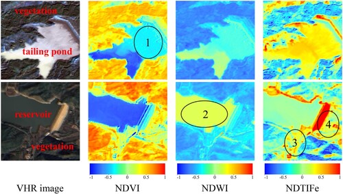
Tailing ponds in the study area are typically located on the mountains or flat lands, and are surrounded by vegetation, including grasses, bushes, and trees (Q. T. Li et al. 2020). Therefore, the Normalized Difference Vegetation Index (NDVI) is calculated using the red and near-infrared bands of VHR images. As a spectral feature, NDVI can distinguish tailing ponds from surrounding vegetation (Z. Q. Guo, Liu, Zheng et al. 2021). Tailing ponds store tailing wastes containing industrial waste water, so, to a degree, tailing ponds are easily confused with water in reservoirs or lakes. To further reduce the error rate caused by water, the Normalized Difference Water Index (NDWI) is calculated using the green and near-infrared bands of VHR images (Ge, Xie, and Meng 2022). The Normalized Difference Tailing Index for Fe-Bearing Minerals (NDTIFe) was proposed by Hao, Zhang, and Yang (2019) and applied to tailing ponds extraction in Huangshi, China. Their experiments proved that NDTIFe could effectively provide enhanced information about tailing ponds. Therefore, in this study, NDTIFe is calculated using the green and near-infrared bands of VHR images and used as one of the HCFs. The three HCFs: NDVI, NDWI, and NDTIFe are concatenated in the channel dimension to obtain the HCF images.

The three HCFs are defined in Equations (1)–(3). To demonstrate the critical contribution that HCFs play in distinguishing tailing ponds from surroundings and reservoirs, three HCFs are calculated for a tailing pond and a reservoir as an example, and the results are shown in Figure 1. NDVI highlights the information on vegetation around both tailing ponds and reservoirs. Furthermore, the NDVI is higher in areas of high tailings concentration than in the reservoir (region 1). The values of NDWI are higher in the reservoir than in the tailing pond (region 2). NDTIFe distinguishes the tailing pond from the surroundings, while this is not obvious for reservoir (regions 3 and 4). Overall, using NDVI, NDWI, and NDTIFe can complement the information on tailing ponds and improve the ability to accurately extract tailing ponds from VHR images. (1) $\mathrm{NDVI}={\displaystyle \frac{B_{\mathrm{Nir}}-B_{\mathrm{Red}}}{B_{\mathrm{Nir}}+B_{\mathrm{Red}}}}$(1) (2) $\mathrm{NDWI}={\displaystyle \frac{B_{\mathrm{Green}}-B_{\mathrm{Nir}}}{B_{\mathrm{Green}}+B_{\mathrm{Nir}}}}$(2) (3) $\mathrm{NDTIFe}={\displaystyle \frac{B_{\mathrm{Red}}-B_{\mathrm{Blue}}}{B_{\mathrm{Green}}+B_{\mathrm{Nir}}}}$(3)

Figure 1. The calculation results of HCFs. The first and second rows show the VHR image, NDVI, NDWI, and NDTIFe of a tailing pond and a reservoir, respectively.

where $B_{\mathrm{Red}}$, $B_{\mathrm{Green}}$, $B_{\mathrm{Blue}}$, $B_{\mathrm{Nir}}$ are the red, green, blue, and near-infrared bands of VHR images, respectively.

2.2. General structure of PSVED

The structure of PSVED proposed in this study is shown in Figure 2, which mainly consists of the encoder and decoder paths. In the encoder path, the HCF images including the NDVI (Z. Q. Guo, Liu, Zheng et al. 2021), NDWI (Ge, Xie, and Meng 2022), and NDTIFe (Hao, Zhang, and Yang 2019) are calculated based on the three index calculation algorithms, respectively. Then, a Pseudo-Siamese VGG is utilized as the encoder. VHR images and HCF images are input into two branches of the Pseudo-Siamese network respectively, and parameters are not shared between the two branches (W. S. Li et al. 2022). In this way, multi-dimensional deep semantic features ($f_{r1}$, $f_{r2}$, $f_{r3}$, $f_{r4}$, $f_{r5}$) and deep semantic features ($f_{s1}$, $f_{s2}$, $f_{s3}$, $f_{s4}$, $f_{s5}$) are extracted from VHR images and HCF images, respectively. And, deep features of the same layers are added to generate the fused features ($f_{e1}$, $f_{e2}$, $f_{e3}$, $f_{e4}$, $f_{e5}$). In the decoder part of the PSVED, the deep features are gradually recovered in size by upsampling, convolution, and skip connections to obtain five features ($f_{d1}$, $f_{d2}$, $f_{d3}$, $f_{d4}$, $f_{d5}$) (Ronneberger, Fischer, and Brox 2015). To alleviate the problem of gradients vanishing or exploding and accelerate the speed of network fitting (Dou et al. 2017), a deep supervision mechanism with custom loss function weights ($\alpha$, $\beta$, $\gamma$) is attached to train the PSVED (H. N. Guo, Su, Tang et al. 2021). The whole detailed process of training and testing for PSVED is given in Table 1. In the subsequent part sections, we present the key network components.

Figure 2. The structure of PSVED. VHR images and HCF images are fed to PSVED, and then the deep features are extracted by Pseudo-Siamese VGG. Finally, the spatial extent of tailing ponds can be obtained by feature decodes and deep supervision mechanism.

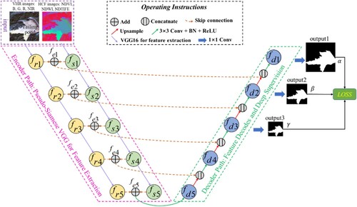
Table 1. Training procedure of the proposed PSVED.

Input:

$\mathrm{imag}{\mathrm{e}}_{\mathrm{r}}$ = $\mathrm{VHR}\mathrm{images}$

$\mathrm{imag}{\mathrm{e}}_{\mathrm{s}}$ = $\mathrm{HCF}\mathrm{images}$

$\mathrm{label}$ = $\mathrm{binary}\mathrm{mask}\mathrm{files}$

Function $\mathrm{Pseudo}\text{-}\mathrm{Siamese}\mathrm{VGG}$($\mathrm{imag}{\mathrm{e}}_{\mathrm{r}}$, $\mathrm{imag}{\mathrm{e}}_{\mathrm{s}}$):

$f_{r1}$, $f_{r2}$, $f_{r3}$, $f_{r4}$, $f_{r5}$ =  $\mathrm{Block}(\mathrm{imag}{\mathrm{e}}_{\mathrm{r}})$

$f_{s1}$, $f_{s2}$, $f_{s3}$, $f_{s4}$, $f_{s5}$ = $\widehat{\mathrm{Block}}(\mathrm{imag}{\mathrm{e}}_{\mathrm{s}})$

$f_{e5}$ = $f_{r5}$ + $f_{s5}$

$f_{d5}$ =  $\mathrm{Con}{\mathrm{v}}_3(f_{e5})$

$\mathrm{For}\mathrm{i}\mathrm{in}2:5\mathrm{do}:$

$f_{e(6-i)}$ =  $f_{r(6-i)}+f_{s(6-i)}$

$f_{d(6-i)}$ = u$p(f_{d(6-i+1)})$

$f_{d(6-i)}$ = $\mathrm{Cat}(f_{d(6-i)},f_{e(6-i)})$

$f_{d(6-i)}$ = $\mathrm{Con}{\mathrm{v}}_3(f_{d(6-i)})$

$\mathrm{if}\mathrm{training}:$

$\mathrm{Loss}=\alpha L(\mathrm{Con}{\mathrm{v}}_1(f_{d1}),\mathrm{label})$ + $\beta L(\mathrm{Con}{\mathrm{v}}_1(f_{d2}),\mathrm{MP}(\mathrm{label}))$+ $\gamma L(\mathrm{Con}{\mathrm{v}}_1(f_{d3}),\mathrm{MP}(\mathrm{label}))$, $\alpha$ + $\beta$ + $\gamma$ = 1

$\widetilde{w_i}$ = $w_i-\alpha (\mathrm{\partial }\mathrm{Loss}/\mathrm{\partial }w)$

return $\widetilde{w_i}$

$\mathrm{if}\mathrm{testing}:$

return $\mathrm{Con}{\mathrm{v}}_1(f_{d1})$

2.3. Pseudo-Siamese VGG for feature extraction

The VHR images after data preprocessing have four multispectral bands: blue, green, red, and near-infrared, while HCF images have three HCFs: NDVI, NDWI, and NDTIFe. VHR images contain rich scene information, while HCF images contain rich spectral information. Neither the early-fusion methods nor the late-fusion methods in the published literatures have achieved a reasonable use of HCFs (Z. Q. Guo, Liu, Zheng et al. 2021; L. H. Wang, Yue, Wang et al. 2020). Therefore, in this study, considering the information gap between the VHR images and HCF images, a Pseudo-Siamese VGG is used to extract multi-dimensional deep scene semantic and spectral semantic features from VHR images and HCF images, respectively (W. S. Li et al. 2022; Wu et al. 2022). A Pseudo-Siamese network is a network architecture similar to a Siamese network. The Pseudo-Siamese network has two independent and equal feature extraction streams, but the weights are not shared (W. S. Li et al. 2022). The two extraction streams can extract more independent and representative deep scene semantic features from VHR images and HCF images. In addition, the multi-dimensional deep scene semantic and deep spectral semantic features are fused at multiple levels to achieve sufficient fusion of information.

VGG is a deep CNN proposed by the Visual Geometry Group of Oxford University in 2014 (Simonyan and Zisserman 2014). Instead of 5 × 5 convolutional layers or 7 × 7 convolutional layers, VGG adopts 3 × 3 convolutional layers. Therefore, the structure of VGG is relatively simple and is popularly used in semantic segmentation to extract deep features (Chaib et al. 2017; Simonyan and Zisserman 2014). In this study, VGG16 is utilized as the feature extractor. VGG16 consists of thirteen convolutional layers and three fully connected layers (Simonyan and Zisserman 2014). In this paper, the three fully connected layers are removed to maintain the size of the feature maps and reduce the loss of spatial information in the tailing ponds extraction task. The structure of the modified VGG16 is shown in Figure 3. The modified VGG16 consists of five convolutional blocks: the first block is composed of two convolutional layers; the second block is composed of a pooling layer and two convolutional layers; the third, fourth and fifth blocks are composed of a pooling layer and three convolutional layers, respectively.

Figure 3. The structure of modified VGG16 which consists of five blocks. Each block consists of convolution layer, batch normalization layer, activation layer and Max-Pooling layer.

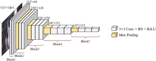
Each convolutional block in the modified VGG16 can extract a deep scene semantic feature from VHR images and a deep spectral semantic feature from HCF images. The five deep scene semantic features and five labeled deep spectral semantic features are labeled as ($f_{r1}$, $f_{r2}$, $f_{r3}$, $f_{r4}$, $f_{r5}$) and ($f_{s1}$, $f_{s2}$, $f_{s3}$, $f_{s4}$, $f_{s5}$), respectively. The five deep features’ channels are 64, 128, 256, 512, and 512 respectively. The deep scene semantic features and deep spectral semantic features of the same layer are added to generate deep semantic features labeled ($f_{e1}$, $f_{e2}$, $f_{e3}$, $f_{e4}$, $f_{e5}$). $f_{ri}$, $f_{si}$, $f_{ei}$ are defined in Equations (4)–(6): (4) $f_{r1}=\mathrm{Bloc}{\mathrm{k}}_1(\mathrm{imag}{\mathrm{e}}_{\mathrm{r}}),f_{ri}=\mathrm{Bloc}{\mathrm{k}}_{\mathrm{i}}(f_{r(i-1)}),\mathrm{i}(2,3,4,5)$(4) (5) $f_{s1}={\widehat{\mathrm{Block}}}_1(\mathrm{imag}{\mathrm{e}}_{\mathrm{s}}),f_{si}={\widehat{\mathrm{Block}}}_{\mathrm{i}}(f_{s(i-1)}),i(2,3,4,5)$(5) (6) $f_{ei}=f_{ri}+f_{si},i(1,2,3,4,5)$(6)

where $\mathrm{Bloc}{\mathrm{k}}_{\mathrm{i}}$ and ${\widehat{\mathrm{Block}}}_{\mathrm{i}}$ denote the $\mathrm{i}\text{-}\mathrm{th}$ convolutional block of the Pseudo-Siamese VGG16, respectively; $\mathrm{imag}{\mathrm{e}}_{\mathrm{r}}$ denotes the VHR images; $\mathrm{imag}{\mathrm{e}}_{\mathrm{s}}$ denotes the HCF images.

2.4. Feature decodes and deep supervision mechanism

The decoder path consists of five layers, each consisting of an upsampling layer and two convolutional layers. Meanwhile, skip connection is utilized to reuse the deep semantic features (Ronneberger, Fischer, and Brox 2015). In other words, in the decoder path, five fused features are obtained by upsampling, convolution, and skip connection, which is labeled ($f_{d1}$, $f_{d2}$, $f_{d3}$, $f_{d4}$, $f_{d5}$) and defined in Equation (7): (7) $f_{d5}=\mathrm{Con}{\mathrm{v}}_3(f_{e5}),f_{di}=\mathrm{Con}{\mathrm{v}}_3(\mathrm{Cat}(\mathrm{up}(f_{d(i+1)}),f_{ei})),i(4,3,2,1)$(7)

where $\mathrm{Con}{\mathrm{v}}_3(\cdot )$ denotes 3 × 3 convolutional layer; $\mathrm{Cat}(\cdot )$ denotes feature concatenated in the channel dimension; $\mathrm{up}(\cdot )$ denotes upsampling layer.

The key to CNN work is using the backpropagation algorithm for weights update to improve the network (C. X. Zhang et al. 2020). The weight update method is defined in Equation (8): (8) $\widetilde{w_i}=w_i-lr\times (\mathrm{\partial }Loss/\mathrm{\partial }w)$(8)

where $\widetilde{w_i}$ is the updated weight; $w_i$ is the weight before the update; $lr$ is the learning rate; $\mathrm{\partial }\mathrm{Loss}/\mathrm{\partial }w$ represents the error gradient of the loss function.

With the increase of network layers, the error gradient transmitted to the convolution layers near the input layer may be too small or too large, resulting in gradients vanishing or exploding (Dou et al. 2017). The problem is alleviated by utilizing a deep supervision mechanism for training the PSVED. Auxiliary classifiers are added to the last three features of the decoder path, and losses are calculated to supervise the model training (Szegedy et al. 2015). The deep supervision mechanism allows the model to be supervised by multiple features, which helps to alleviate the adverse effects of changes in unstable gradients, handle the problem of gradients vanishing or exploding, and accelerate the convergence speed (Dou et al. 2017; C. X. Zhang et al. 2020). The loss of PSVED is defined in Equation (9): (9) $\mathrm{Loss}=\alpha L(\mathrm{Con}{\mathrm{v}}_1(f_{d1}),\mathrm{label})+\beta L(\mathrm{Con}{\mathrm{v}}_1(f_{d2}),\mathrm{MP}(\mathrm{label}))+\gamma L(\mathrm{Con}{\mathrm{v}}_1(f_{d3}),\mathrm{MP}(\mathrm{label}))$(9)

where $L(\cdot )$ denotes the loss function of PSVED; $\mathrm{label}$ represents the binary mask file of tailing pond; $\mathrm{MP}(\cdot )$ denotes Max-Pooling operation; $\mathrm{Con}{\mathrm{v}}_1(\cdot )$ denotes 1 × 1 convolutional layer; $\alpha$, $\beta$, and $\gamma$ are the weights of the three parts, respectively, and $\alpha$ + $\beta$ + $\gamma$ = 1.

In existing studies, the balanced deep supervision strategy is commonly applied (D. C. Wang, Chen, Jiang et al. 2021; C. X. Zhang et al. 2020). However, due to the different fineness of the output features of different layers, the output results of different layers contribute differently to the extraction results of tailing ponds, making it challenging to maximize the effectiveness of the deep supervision mechanism (L. Li et al. 2018). Therefore, a progressive deep supervision strategy is proposed, and the weights are determined according to the ratio of the edge lengths of output features of different layers. Such a strategy can fully use the output deep features of different layers and optimize the network weight by backpropagating the loss calculated to the earlier network layers, which can effectively improve the performance of PSVED. Since the ratio of edge lengths of $f_{d1}$, $f_{d2}$, and $f_{d3}$ is 4:2:1, the parameters $\alpha$, $\beta$, and $\gamma$ are set to 4/7, 2/7 and 1/7, respectively.

2.5. Technical route

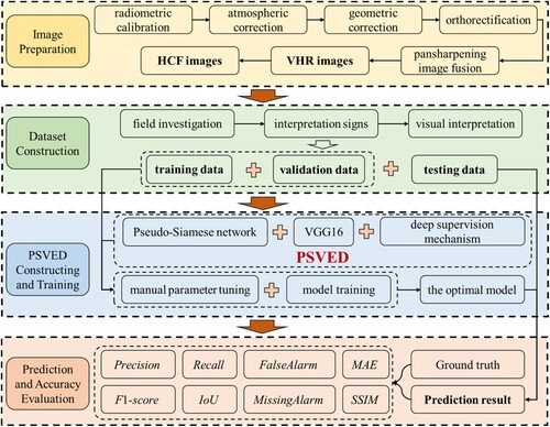
The research in this paper consists of four steps, which is shown in Figure 4.

1. Image Preparation: The VHR images are obtained through data preprocessing, and the HCF images are obtained through index calculation algorithms based on the VHR images.

2. Dataset Construction: The tailing ponds extraction dataset is constructed through field investigation and visual interpretation, and then is divided into training, validation and testing data.

3. PSVED Constructing and Training: The PSVED is developed by integrating the Pseudo-Siamese network, VGG16, and deep supervision mechanism, and is trained with a manual tuning method to obtain the optimal extraction model.

4. Prediction and Accuracy Evaluation: The optimal extraction model is utilized to extract the tailing ponds and is quantitatively evaluated with the accuracy of the extraction results.

Figure 4. Technical route of the research in this paper, encompassing four main parts: Image Preparation, Dataset Construction, PSVED Construction and Training, and Prediction and Accuracy Evaluation.

3. Experiments

3.1. Study area and data

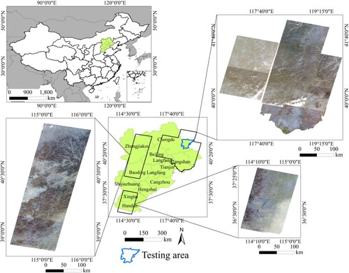
In this study, a public tailing ponds extraction dataset (TPSet) was self-produced for tailing ponds extraction. The coverage area of TPSet is located in the Hebei Province of China and includes mainly Tangshan, Chengde, Baoding, etc. The reserves of the iron ore resources of Hebei are ranked third in China. The active mining industry, especially iron ore mining, leads to several thousands of tailing ponds, which has been becoming a significant dangerous problem (Lyu et al. 2021). The images acquired by Gaofen-6 Panchromatic &·Multispectral Scanners (PMS) were used in this study. The spatial resolution of the panchromatic (PAN) band of the Gaofen-6 is 2 m, and the spatial resolution of the multispectral (MS) bands is 8 m (M. Y. Li et al. 2021). The images were provided by China Center for Resources Satellite Date and Application and the Aerospace Information Research Institute under the Chinese Academy of Sciences. The location and image coverage of the study area are shown in Figure 5.

Figure 5. Location of the study area in Hebei Province, China. The VHR images displayed in the figure were obtained after preprocessing.

The preprocessing steps of Gaofen-6 images include radiometric calibration, atmospheric correction, geometric correction, orthorectification, and pansharpening image fusion (Y. Zhang 2002). All the operations were implemented through PIE-Basic 6.0 software, which is a professional tool for processing remotely sensed images, and has been widely used for image preprocessing (Wang and Wang 2022). The images after preprocessing include four bands of R, G, B, and NIR, with a spatial resolution of 2 m. In addition, all VHR images displayed and used for HCFs calculation in this paper were obtained after preprocessing.

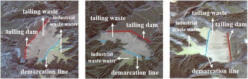
The tailing ponds mask files were generated by visual interpretation of VHR images and the assistance of field investigation. Specifically, the interpretation signs were established according to color and shape (C. S. Wang, Chang, Zhao et al. 2020). VHR image interpretation signs of tailing ponds include:

1. From the perspective of color: the tailing ponds mainly consist of tailing waste and industrial waste water. From true-color synthesis VHR images, in the higher terrain areas, the concentration of tailing waste is higher and usually appears grayish-white. In the lower terrain areas, the concentration of industrial waste water is higher and usually appears yellow-green. Furthermore, there is a clear demarcation line between the two areas.

2. From the perspective of shape: there are apparent straight tailing dams as the tailing ponds are constructed artificially (Figure 6).

Figure 6. Examples of tailing ponds, containing tailing dam, tailing waste, industrial waste and demarcation line.

Limited to the computer computing performance, VHR images need to be divided into image patches before feeding them into the network. The operation has been widely used in ground objects extraction based on deep learning methods. This will have adverse effects on the tailing ponds extraction accuracy to some degree, because the incomplete edge structure and the lack of global information of tailing ponds (Ding, Zhang, and Bruzzone 2020; H. Wang, Chen, Zhang et al. 2022). However, it is consistent with the practical application, i.e. the distribution of tailing ponds in the test area is unknown. Through cropping, the TPSet contains 1389 images and binary mask files with a size of 512 × 512 pixels. The data was randomly divided in a ratio of 7:3, with 70% samples used for model training and the remaining 30% for model validation. To improve the generalization ability of the model, three simple and widely used data augmentation methods including image rotation, image flipping and image blurring, were employed and made the number of training data reach 4000 (S. H. Du, Xing, Li et al. 2022; M. Y. Li et al. 2021; Lyu et al. 2021; C. X. Zhang et al. 2020). A county-scale area was selected for model testing, and the testing data contains 3564 images and binary mask files with a size of 512 × 512 pixels. In particular, the testing data had no intersection with the training and validation data.

3.2. Experimental configuration

The experiments were implemented using a desktop computer with Intel Xeon Gold 5118, 16.0 GB memory, and NVIDIA GeForce RTX2080Ti. All algorithms were performed using Python language (v3.6.5) on the PyCharm platform (Community Edition 2020.2.1 × 64). The deep learning framework was pytorch (v1.7.0 + cu110). The method of manual parameter tuning was employed to search for a suitable learning rate and the value was set to 0.005. Some published works have proven that relatively larger batch size is beneficial for higher model accuracy (Radiuk 2017). However, limited to computer memory and data volume, the batch size was set to 4 in this study. The Adam function was selected as the parameter optimizer since it is robust and well-suited to a wide range of non-convex optimization problems in deep learning. The Cross-Entropy loss function was employed to measure the fitting effect of the model. Besides these parameters, to train the model until the loss curve tends to be smooth, the maximum number of training iteration epochs was set to 200. To evaluate the effectiveness of the proposed PSVED, five typical methods, including MsanlfNet (Bai et al. 2022), LANet (Ding, Tang, and Bruzzone 2021), DeepLabv3+ (Chen et al. 2018), U-Net (Ronneberger, Fischer, and Brox 2015), and MLC (Orimoloye and Ololade 2020) have been implemented in the experiments. Especially, all of the above methods use both VHR images and HCF images. In addition, among them, MLC belongs to traditional machine learning methods and the others belong to deep learning methods.

In this study, Mean Absolute Error (MAE) and Structural Similarity Index Measure (SSIM) were used to evaluate the similarity of the predicted probability map with the ground truth and test the significance of the methods. $\mathrm{MAE}$ and $\mathrm{SSIM}$ are defined as $\mathrm{MAE}$: $\sum _{i=1}^m|P_i-G_i|/m$ and $\mathrm{SSIM}$: $((2\times u_P\times u_G+C_1)(2\times {\sigma }_{PG}+C_2))/((u_P^2+u_G^2+C_1)({\delta }_P^2+{\delta }_G^2+C_2))$, where $P$ denotes the predicted probability map; $G$ denotes the ground truth; $\mathrm{m}$ is the number of pixels; $u_P$ and $u_G$ represent the means of $P$ and $G$, respectively; ${\delta }_{\mathrm{P}}^2$ and ${\delta }_{\mathrm{G}}^2$ represent the variances of $P$ and $\mathrm{G}$, respectively; ${\sigma }_{\mathrm{PG}}$ denotes the covariance of $P$ and $G$. Generally, $C_1=(0.01\times L{)}^2$, $C_2=(0.03\times L{)}^2$, and $L$ is the maximum image value (Xiong et al. 2020).

In addition, the pixel-based and the object-based evaluation metrics were used to evaluate the accuracy of the prediction results (S. H. Du, Xing, Li et al. 2022). The pixel-based evaluation metrics, including $\mathrm{Precision}$: $\mathrm{T}{\mathrm{P}}_{\mathrm{p}}/(\mathrm{T}{\mathrm{P}}_{\mathrm{p}}+\mathrm{F}{\mathrm{P}}_{\mathrm{p}})$, $\mathrm{Recall}$: $\mathrm{T}{\mathrm{P}}_{\mathrm{p}}/(\mathrm{T}{\mathrm{P}}_{\mathrm{p}}+\mathrm{F}{\mathrm{N}}_{\mathrm{p}})$, $\mathrm{F}1\text{-}\mathrm{score}$: $2\cdot \mathrm{PrecisionRecall}/(\mathrm{Precision}+\mathrm{Recall})$, and $(\mathrm{Intersection}\mathrm{over}\mathrm{Union})\mathrm{IoU}$: $\mathrm{T}{\mathrm{P}}_{\mathrm{p}}/(\mathrm{T}{\mathrm{P}}_{\mathrm{p}}+\mathrm{F}{\mathrm{P}}_{\mathrm{p}}+\mathrm{F}{\mathrm{N}}_{\mathrm{p}})$, where $\mathrm{T}{\mathrm{P}}_{\mathrm{p}}$ represents the number of tailing pond pixels that are correctly extracted; $\mathrm{F}{\mathrm{P}}_{\mathrm{p}}$ represents the number of background pixels that are extracted as tailing pond pixels; $\mathrm{F}{\mathrm{N}}_{\mathrm{p}}$ represents the number of tailing pond pixels that are extracted as background. In terms of object-based evaluation, $\mathrm{FalseAlarm}$: $\mathrm{F}{\mathrm{P}}_{\mathrm{o}}/(\mathrm{T}{\mathrm{P}}_{\mathrm{o}}+\mathrm{F}{\mathrm{P}}_{\mathrm{o}})$ and $\mathrm{MissingAlarm}$: $\mathrm{F}{\mathrm{N}}_{\mathrm{o}}/(\mathrm{T}{\mathrm{P}}_{\mathrm{o}}+\mathrm{F}{\mathrm{N}}_{\mathrm{o}})$ are used to quantitatively evaluate the extracted results, where $\mathrm{T}{\mathrm{P}}_{\mathrm{o}}$, $\mathrm{F}{\mathrm{P}}_{\mathrm{o}}$, $\mathrm{F}{\mathrm{N}}_{\mathrm{o}}$ have the same meaning as $\mathrm{T}{\mathrm{P}}_{\mathrm{p}}$, $\mathrm{F}{\mathrm{P}}_{\mathrm{p}}$, $\mathrm{F}{\mathrm{N}}_{\mathrm{p}}$, but they express the number of objects rather than the number of pixels.

3.3. Experimental results

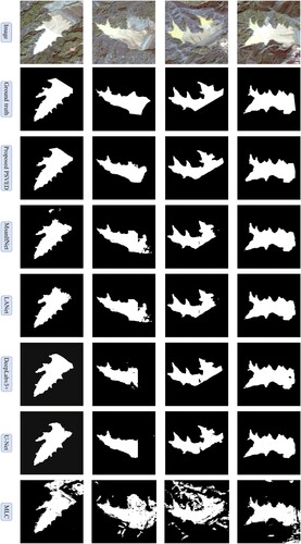
The effectiveness of the proposed PSVED in the tailing ponds extraction task was evaluated using experiments on the TPSet. The extraction visualization results for some individual tailing ponds of six methods are shown in Figure 7. In general, Figure 7 proves that all methods can extract these tailing ponds. However, the results extracted by MLC contain the most incorrect extracted regions and holes than that in the other methods (i.e. deep learning methods). For the deep learning methods, the results extracted by the proposed PSVED best match the ground truth with less information loss, more complete boundaries, and higher internal compactness than that in MsanlfNet, LANet, DeepLabv3+, and U-Net.

Figure 7. The extraction visualization results for some individual tailing ponds. The white area signifies the spatial extent of tailing ponds, while the black area represents the background (the following Figures 8 and 10 are the same).

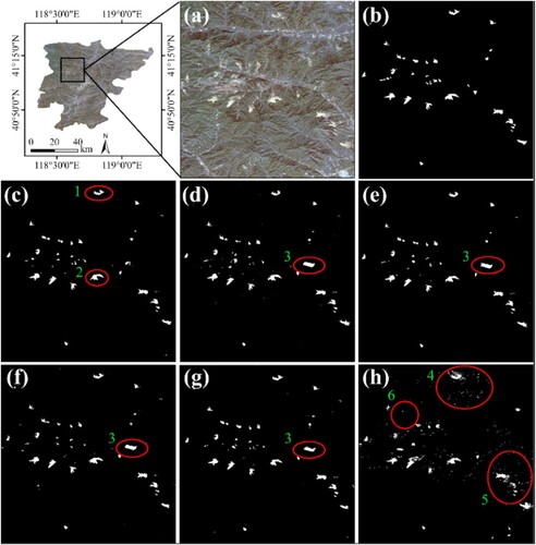
The extraction visualization results in a large-scale area are shown in Figure 8. Figure 8 demonstrates that the extraction results of the proposed PSVED best match the ground truth, retaining more complete details (regions 1 and 2). In addition, as shown in Figure 8(d–g), MsanlfNet, LANet, DeepLabv3+, and U-Net have the problem of extracting water as tailing ponds (region 3), while the proposed method alleviates this problem. Due to many incorrect and missed extractions (regions 4, 5, and 6), the results of MLC have the largest error deviation from the ground truth.

Figure 8. The extraction visualization results on a large-scale area. (a) VHR image, (b) Ground truth, (c) PSVED, (d) MsanlfNet, (e) LANet, (f) DeepLabv3+, (g) U-Net, (h) MLC.

The significance test of the six methods was conducted and the results are shown in Table 2. PSVED achieved the highest $\mathrm{SSIM}$ (0.8895) and the minimum $\mathrm{MAE}$ (0.0043). The sub-optimal method is LANet, which achieves $\mathrm{MAE}$ of 0.0058 and $\mathrm{SSIM}$ of 0.8646. Among all the models, MLC had the poorest performance with $\mathrm{MAE}$ of 0.0520 and $\mathrm{SSIM}$ of 0.6650.

Table 2. Significance test results on TPSet.

Method	$\mathrm{MAE}\downarrow$	$\mathrm{SSIM}\uparrow$
PSVED	0.0043	0.8895
MsanlfNet	0.0061	0.8432
LANet	0.0058	0.8646
DeepLabv3+	0.0065	0.8241
U-Net	0.0060	0.8568
MLC	0.0520	0.6650

$\uparrow$: The higher the value, the better the extraction performance. $\downarrow$: The lower the value, the better the extraction performance. The bolded is the best result. The following tables are the same.

To further evaluate the performance of the proposed PSVED, the pixel-based quantitative evaluation was conducted, and the results are listed in Table 3. The proposed PSVED achieves the best performance, with the highest accuracy of 86.86% ($\mathrm{F}1\text{-}\mathrm{score}$) and 76.77% ($\mathrm{IoU}$). Significantly higher than the other deep learning methods and MLC. The improvement by PSVED over the sub-optimal LANet is 4.42 percentage points ($\mathrm{F}1\text{-}\mathrm{score}$) and 6.67 percentage points ($\mathrm{IoU}$). The MLC has the lowest accuracy among the six methods at 58.32% ($\mathrm{F}1\text{-}\mathrm{score}$), and 41.16% ($\mathrm{IoU}$).

Table 3. Pixel-based quantitative evaluation results on TPSet.

Method	$\mathrm{Precision}\uparrow$	$\mathrm{Recall}\uparrow$	$\mathrm{F}1\text{-}\mathrm{score}\uparrow$	$\mathrm{IoU}\uparrow$
PSVED	87.71%	86.03%	86.86%	76.77%
MsanlfNet	75.84%	81.37%	78.51%	64.62%
LANet	82.97%	81.92%	82.44%	70.13%
DeepLabv3+	73.93%	82.47%	77.97%	63.89%
U-Net	79.84%	81.56%	80.69%	67.63%
MLC	57.41%	59.25%	58.32%	41.16%

The proposed PSVED was trained and tested using the unaugmented and augmented data to evaluate the effectiveness of the three data augmentation methods. The quantitative evaluation results are shown in Table 4. After data augmentation, all the evaluation metrics have been improved, which indicates that the three data augmentation methods employed in this study is simple but practical. In addition, it can be seen from Tables 3 and 4 that, the quantitative evaluation results of PSVED with unaugmented data are superior to those of the other tested methods with augmented data. This further illustrates the effectiveness and practicality of the proposed PSVED.

Table 4 . Quantitative evaluation results on the effectiveness of data augmentation methods.

Method	$\mathrm{Precision}\uparrow$	$\mathrm{Recall}\uparrow$	$\mathrm{F}1\text{-}\mathrm{score}\uparrow$	$\mathrm{IoU}\uparrow$
PSVED with unaugmented data	85.62%	84.37%	84.99%	73.89%
PSVED with augmented data	87.71%	86.03%	86.86%	76.77%

The object-based quantitative evaluation results of different methods are shown in Table 5. The results of MLC have the most incorrect and missed extraction objects, and the values of $\mathrm{FalseAlarm}$ (36.36%) and $\mathrm{MissingAlarm}$ (40.68%) are significantly higher than the other five deep learning methods, which further illustrates the difficulty for MLC to achieve high-accuracy tailing ponds extraction. Among the five deep learning methods, the $\mathrm{FalseAlarm}$ and $\mathrm{MissingAlarm}$ of the proposed PSVED are the lowest (both are 8.47%), i.e. the least number of incorrect and missed extraction tailing ponds objects.

Table 5. Object-based quantitative evaluation results on TPSet.

Method	$\mathrm{FalseAlarm}\downarrow$	$\mathrm{MissingAlarm}\downarrow$
PSVED	8.47%	8.47%
MsanlfNet	15.25%	15.25%
LANet	16.13%	11.86%
DeepLabv3+	12.07%	13.56%
U-Net	19.05%	13.56%
MLC	36.36%	40.68%

In summary, through the above analysis, it can be concluded that the proposed method is the model with the best comprehensive performance for tailing ponds extraction.

The time consumed by different methods in the same machine is compared. Since the training and testing of MLC are significantly different from the other five deep learning methods, only the five deep learning methods are compared in time consumption. The time consumption of the five methods is listed in Table 6. Overall, it can be inferred that the time consumption of all five methods is located at the same level. In detail, the time consumption of U-Net is the shortest, while that of DeepLabv3 + is the longest. Since PSVED contains more trainable parameters, it takes longer to train and test, and only outperforms DeepLabv3 + .

Table 6. The time consumption of the five methods.

Method	Number of parameters	Time consumption for model training (s/per epoch)	Time consumption for model testing (s)
PSVED	39848774	754	223
MsanlfNet	36466754	681	214
LANet	23795468	648	190
DeepLabv3+	54700722	827	244
U-Net	17263683	571	165

4. Discussion

4.1. The effectiveness of different loss function weights

In this study, a deep supervision mechanism is introduced to train the PSVED, and the weights of the loss function are $\alpha$, $\beta$, and $\gamma$ respectively. As such, experiments were conducted to evaluate the performance of different loss function weights to explore the optimal combination of loss function weights. Method ($\mathrm{I}$) adopts the un-deep supervised strategy, i.e. only the $f_{d1}$ is utilized for training the PSVED, where $\alpha$ = 1, $\beta$ = 0, $\gamma$ = 0. Method ($\mathrm{II}$) adopts the balanced deep supervision strategy, where $\alpha$ = $\beta$ = $\gamma$ = 1/3. Method ($\mathrm{III}$) adopts the progressive deep supervision strategy, where $\alpha$ = 4/7, $\beta$ = 2/7, $\gamma$ = 1/7. The weight ratio of Method ($\mathrm{III}$) is equal to the ratio of edge lengths of $f_{d1}$, $f_{d2}$, and $f_{d3}$ (512: 256: 128 = 4: 2: 1)

Table 7 shows the quantitative evaluation results of the three methods. Method ($\mathrm{III}$) achieves the best performance, with the highest accuracy of 86.86% ($\mathrm{F}1\text{-}\mathrm{score}$) and 76.77% ($\mathrm{IoU}$), which shows an improvement in accuracy of 0.97 percentage points ($\mathrm{F}1\text{-}\mathrm{score}$) and 1.50 percentage points ($\mathrm{IoU}$) compared to the sub-optimal Method ($\mathrm{II}$). Moreover, there is a significant improvement in accuracy compared to Method ($\mathrm{I}$).

Table 7. Quantitative evaluation with the different loss function weights.

Method	($\alpha$, $\beta$, $\gamma$)	$\mathrm{Precision}\uparrow$	$\mathrm{Recall}\uparrow$	$\mathrm{F}1\text{-}\mathrm{score}\uparrow$	$\mathrm{IoU}\uparrow$
$(\mathrm{I}$)	(1,0,0)	83.55%	84.93%	84.23%	72.76%
$(\mathrm{II}$)	(1/3,1/3,1/3)	86.60%	85.19%	85.89%	75.27%
$(\mathrm{III}$)	(4/7,2/7,1/7)	87.71%	86.03%	86.86%	76.77%

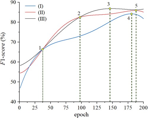
The $\mathrm{F}1\text{-}\mathrm{score}$ changing curves of the three methods during model training are shown in Figure 9. In general, during the training process, the $\mathrm{F}1\text{-}\mathrm{score}$ gradually increases. It can be seen that Method ($\mathrm{I}$) has the fastest rate of improvement until point 1 (epoch = 37), but then the rate slows down significantly and finally reaches the highest accuracy at point 4 (epoch = 181). Both Method ($\mathrm{II}$) and Method ($\mathrm{III}$) maintain approximately the same rate of improvement until point 2 (epoch = 97), and the rate slows down after that, especially for Method ($\mathrm{II}$). Eventually, Method ($\mathrm{III}$) reaches the highest accuracy at point 3 (epoch = 146), and Method ($\mathrm{II}$) reaches the highest accuracy at point 5 (epoch = 188). The results indicate that deep supervision combined with appropriate loss function weights can significantly improve the accuracy and accelerate the convergence speed in the tailing ponds extraction task.

Figure 9. The training process of different loss function weights. Points 1–5 represent the special nodes of the three methods in the training process.

4.2. Ablation study

In this study, not only VHR images but also HCF images are used for tailing ponds extraction. In addition, the deep supervision mechanism is used for training the model. Ablation experiments were conducted to evaluate the effectiveness of HCF images and deep supervised mechanism for tailing ponds extraction. The results of the ablation experiments are shown in Table 8. It can be seen that all of them help improve the performance of tailing ponds extraction. The $\mathrm{F}1\text{-}\mathrm{score}$ and $\mathrm{IoU}$ of Method $\mathrm{B}$ are 1.57 percentage points and 2.22 percentage points higher than that of Method $\mathrm{A}$, respectively. The $\mathrm{F}1\text{-}\mathrm{score}$ and $\mathrm{IoU}$ of Method $\mathrm{C}$ are 1.06 percentage points and 1.43 percentage points higher than that of Method $\mathrm{A}$, respectively. Most importantly, the Method $\mathrm{D}$ which incorporates both the HCF images and the deep supervised mechanism achieves the highest accuracy of 86.86% ($\mathrm{F}1\text{-}\mathrm{score}$) and 76.77% ($\mathrm{IoU}$).

Table 8. Quantitative evaluation of ablation study.

Method	HCF images	Deep supervision mechanism	$\mathrm{Precision}\uparrow$	$\mathrm{Recall}\uparrow$	$\mathrm{F}1\text{-}\mathrm{score}\uparrow$	$\mathrm{IoU}\uparrow$
$\mathrm{A}$	–	–	81.39%	83.96%	82.66%	70.44%
$\mathrm{B}$	√	–	83.55%	84.93%	84.23%	72.76%
$\mathrm{C}$	–	√	82.29%	85.02%	83.63%	71.87%
$\mathrm{D}$	√	√	87.71%	86.03%	86.86%	76.77%

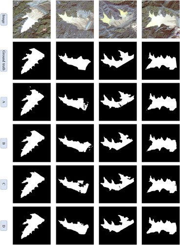
The extraction visualization results of the ablation experiments are shown in Figure 10. First, it can be seen that the results of both Method $\mathrm{B}$ and Method $\mathrm{C}$ are significantly improved with less information loss compared to Method $\mathrm{A}$, which indicates that both the deep supervision mechanism and the HCF images are helpful for the tailing ponds extraction task. Second, it is also evident that Method $\mathrm{B}$ and Method $\mathrm{D}$ with HCF images, have fewer holes and missed extraction regions than Method $\mathrm{A}$ and Method $\mathrm{C}$. This further indicates that the utilization of HCF images enhances the information about tailing ponds and expands the difference with the surroundings and is beneficial to the task of tailing ponds extraction.

Figure 10. The extraction visualization results of the ablation study.

4.3. Comparison of different HCF images utilization methods

The Pseudo-Siamese network extracts deep multidimensional features from VHR and HCF images. To evaluate whether the Pseudo-Siamese network can fully use the HCF images for tailing ponds extraction, a comparative experiment has been conducted between PSVED and the Visual Geometry Group Encoder-Decoder Network (VED). The VED first concatenates the VHR images and HCF images in the channel dimension to obtain the concatenated images with a band number of 7. Then the modified VGG16 is utilized to extract the deep multidimensional features. Like PSVED, VED also adopts the deep supervised mechanism with the same loss function weights.

Table 9 shows the quantitative evaluation results between PSVED and VED. Compared with VED, the accuracy of PSVED has improved by 3.53 percentage points $(\mathrm{F}1\text{-}\mathrm{score})$ and 5.35 percentage points ($\mathrm{IoU}$). The difference in accuracy is because VHR images contain rich spatial scene information, and HCF images contain rich spectral information of tailing ponds (Ge, Xie, and Meng 2022; Z. Q. Guo, Liu, Zheng et al. 2021; Hao, Zhang, and Yang 2019). It should be noted that there is obvious information gap between the two images. VED directly concatenates VHR images with HCF images and then uses CNN to directly extract the deep features of the concatenated images, but there are two problems in this operation. On the one hand, it is difficult to achieve sufficient images fusion by direct concatenation because of the obvious information gap between the two images. On the other hand, it is difficult to provide deep features of individual images to help image reconstruction in the decoder path. PSVED extracts the deep features of VHR images and HCF images respectively with Pseudo-Siamese architecture, and could obtain highly representative deep scene semantic and spectral semantic features. The two deep features are fused in layers in the encoder path and connected to the feature in the decoder path through skip connection. This method can make full use of the extracted deep features to reconstruct the spatial extent feature map of the tailing ponds.

Table 9. Quantitative evaluation of different HCF utilization methods.

Method	$\mathrm{Precision}\uparrow$	$\mathrm{Recall}\uparrow$	$\mathrm{F}1\text{-}\mathrm{score}\uparrow$	$\mathrm{IoU}\uparrow$
PSVED	87.71%	86.03%	86.86%	76.77%
VED	82.68%	83.99%	83.33%	71.42%

4.4. Comparison with different backbones

To evaluate the effectiveness of VGG16 for tailing ponds extraction, several feature extractors, including ResNet101 (He et al. 2016), Xception (Chollet 2017), and MobileNetV2 (Sandler et al. 2018) have been implemented in the comparative experiments. It is worth noting that these four methods adopt the Pseudo-Siamese architecture to extract multi-dimensional deep features from VHR images and HCF images, respectively. It can be seen from Table 10 that the VGG16 has the best accuracy with 2.39 percentage points ($\mathrm{F}1\text{-}\mathrm{score}$), 3.66 percentage points ($\mathrm{IoU}$) higher than the sub-optimal ResNet101. The possible reason is that ResNet101 (101 residual blocks), Xception (34 SeparalbeConv modules), and MobileNetV2 (17 Inverted residuals modules) contain deeper network layers compared to VGG16 (only 13 convolutional layers). Although deeper networks are able to extract deeper features, they can also lead to more information loss in the tailing ponds extraction task. The HCF images can compensate for the lack of information in the VHR images. With the aid of the HCF images, high-accuracy tailing ponds extraction can be achieved by VGG16 which contains fewer layers (only 13 convolutional layers).

Table 10. Quantitative evaluation of different backbones.

Method	$\mathrm{Precision}\uparrow$	$\mathrm{Recall}\uparrow$	$\mathrm{F}1\text{-}\mathrm{score}\uparrow$	$\mathrm{IoU}\uparrow$
VGG16	87.71%	86.03%	86.86%	76.77%
ResNet101	84.25%	84.69%	84.47%	73.11%
Xception	82.07%	83.75%	82.90%	70.79%
MobileNetV2	81.56%	83.01%	82.28%	69.89%

4.5. Limitations and possible improvements

The proposed PSVED has achieved higher accuracy on tailing ponds extraction, which has been proved in the experiments, but there is still content worth studying to improve the accuracy further.

1. Usability analysis of the method: Theoretically, the proposed PSVED is generally applicable and can be applied to extract the spatial extent of tailing ponds in different regions. However, the proposed method still leaves room for improvement, which is mainly in the selection and use of HCFs. The HCFs used in this study are NDVI, NDWI and NDTIFe, all designed for tailing ponds in the study area. However, in other regions such as the western part of China, where the vegetation is sparse (The NDVI surrounding tailing ponds is lower than that in the study area), or in regions such as the Loess Plateau in north-central China where not only the vegetation is sparse, but also the sand content of the reservoirs may be high (The NDVI surrounding the tailing ponds and the NDWI in the reservoirs are both lower than those in the study area), the HCFs mentioned above may not be applicable. Hence, to address this problem, in the follow-up work, the HCFs will be selected for different regions and will be validated.

2. Further optimization of the method: The proposed PSVED has many trainable parameters, increasing the time consumption. Therefore, one of the research directions will be to reduce the model size and the consumption of computing resources by pruning operations (Z. Liu et al. 2017).

3. Further expansion of the study area: Although the study area of this paper is part of Hebei province, the number of tailing pond samples in TPSet is sufficient and representative. Therefore, we concluded that it is possible to implement tailing ponds extraction throughout Hebei province region with TPSet. In the follow-up work, tailing ponds extraction should be implemented throughout Hebei province and even throughout China. In addition, the pruned model should be deployed on a cloud platform to improve the efficiency of tailing ponds extraction in a large area.

5. Conclusions

Automatic tailing ponds extraction from VHR images is essential for mineral resource management. For this purpose, PSVED with an encoder-decoder structure is proposed in this paper. The HCF images are calculated in the encoder path, and a Pseudo-Siamese VGG16 is utilized to extract multidimensional deep semantic features from VHR images and HCF images, respectively. In the decoder path, the size of the features is recovered by operations such as upsampling, convolution, and skip connection. Furthermore, a deep supervision mechanism with custom loss function weights is utilized for training the model. The experiments have been conducted on the self-made TPSet. The results show that the proposed PSVED achieves the best visual performance and accuracy for extracting tailing ponds in all the tested methods. Moreover, the time consumption of the proposed method keeps the same level. Some conclusions also have been reached:

1. HCF images enhance the information about tailing ponds and expand the difference with the surroundings. The multi-dimensional deep semantic features extracted from VHR images and HCF images with Pseudo-Siamese VGG help achieve high accuracy extraction of tailing ponds.

2. Deep supervision mechanism with the progressive deep supervision strategy is more conducive to handling the problem of gradients vanishing or exploding, and accelerating the convergence speed in the task of tailing ponds extraction.

In the future, exploiting more HCFs and expanding the study area need continued research.

Disclosure statement

No potential conflict of interest was reported by the author(s).

Data availability statement

To promote more methods to be investigated for higher accuracy, the TPSet used in this paper has been provided freely. In the data package, there are four data subsets. (1) The training data includes the sub-images and binary mask files (1: pixels of tailing ponds; 0: pixels of non-tailing ponds) (https://figshare.com/s/8a0422b5083b594a2950). (2) The testing data includes the sub-images and binary mask files (1: pixels of tailing ponds; 0: pixels of non-tailing ponds) (https://figshare.com/s/5f98fd97c6dd35a68efb).

Additional information

Funding

This work was supported by the National Key Research and Development Program [grant number: 2022YFF1303301]; The Open Foundation of the Key Laboratory of Coupling Process and Effect of Natural Resources Elements [grant number: 2022KFKTC001]; The National Natural Science Foundation of China [grant number: 42271480]; The Fundamental Research Funds for the Central Universities [grant number: 2023ZKPYDC10, BBJ2023026].

References

- Bai, L., X. Y. Lin, Z. Ye, D. L. Xue, C. Yao, and M. Hui. 2022. “MsanlfNet: Semantic Segmentation Network with Multiscale Attention and Nonlocal Filters for High-Resolution Remote Sensing Images.” IEEE Geoscience and Remote Sensing Letters 19:1–5. https://doi.org/10.1109/lgrs.2022.3185641.
- Chaib, S., H. Liu, Y. F. Gu, and H. X. Yao. 2017. “Deep Feature Fusion for VHR Remote Sensing Scene Classification.” IEEE Transactions on Geoscience and Remote Sensing 55 (8): 4775–4784. https://doi.org/10.1109/TGRS.2017.2700322.
- Chen, L. C., Y. K. Zhu, G. Papandreou, F. Schroff, and H. Adam. 2018. “Encoder-Decoder with Atrous Separable Convolution for Semantic Image Segmentation.” In Proceedings of the European Conference on Computer Vision (ECCV). https://doi.org/10.1007/978-3-030-01234-2_49.
- Cheng, D. Q., Y. F. Cui, Z. H. Li, and J. Iqbal. 2021. “Watch Out for the Tailings Pond, a Sharp Edge Hanging Over Our Heads: Lessons Learned and Perceptions from the Brumadinho Tailings Dam Failure Disaster.” Remote Sensing 13 (9): 1775. https://doi.org/10.3390/rs13091775.
- Chollet, F. 2017. “Xception: Deep Learning with Depthwise Separable Convolutions.” 30th IEEE/CVF Conference on Computer Vision and Pattern Recognition (CVPR). https://doi.org/10.1109/CVPR.2017.195.
- Ding, L., H. Tang, and L. Bruzzone. 2021. “LANet: Local Attention Embedding to Improve the Semantic Segmentation of Remote Sensing Images.” IEEE Transactions on Geoscience and Remote Sensing 59 (1): 426–435. https://doi.org/10.1109/TGRS.2020.2994150.
- Ding, L., J. Zhang, and L. Bruzzone. 2020. “Semantic Segmentation of Large-Size VHR Remote Sensing Images Using a Two-Stage Multiscale Training Architecture.” IEEE Transactions on Geoscience and Remote Sensing 58 (8): 5367–5376. https://doi.org/10.1109/TGRS.2020.2964675.
- do Carmo, F. F., L. H. Y. Kamino, R. Tobias, I. C. de Campos, F. F. do Carmo, G. Silvino, K. de Castro, et al. 2017. “Fundão Tailings dam Failures: The Environment Tragedy of the Largest Technological Disaster of Brazilian Mining in Global Context.” Perspectives in Ecology and Conservation 15 (3): 145–151. https://doi.org/10.1016/j.pecon.2017.06.002.
- Dou, Q., L. Q. Yu, H. Chen, Y. M. Jin, X. Yang, J. Qin, and P. A. Heng. 2017. “3D Deeply Supervised Network for Automated Segmentation of Volumetric Medical Images.” Medical Image Analysis 41:40–54. https://doi.org/10.1016/j.media.2017.05.001.
- Du, Z. Y., L. L. Ge, A. H. M. Ng, Q. G. Z. Zhu, F. G. Horgan, and Q. Zhang. 2020. “Risk Assessment for Tailings Dams in Brumadinho of Brazil Using InSAR Time Series Approach.” Science of the Total Environment 717:137125. https://doi.org/10.1016/j.scitotenv.2020.137125.
- Du, S. H., W. Li, J. Li, S. H. Du, C. Y. Zhang, and Y. Q. Sun. 2022. “Open-pit Mine Change Detection from High Resolution Remote Sensing Images Using DA-UNet++ and Object-Based Approach.” International Journal of Mining, Reclamation and Environment 36 (7): 512–535. https://doi.org/10.1080/17480930.2022.2072102.
- Du, S. H., J. H. Xing, J. Li, S. H. Du, C. Y. Zhang, and Y. Q. Sun. 2022. “Open-Pit Mine Extraction from Very High-Resolution Remote Sensing Images Using OM-DeepLab.” Natural Resources Research 31 (6): 3173–3194. https://doi.org/10.1007/s11053-022-10114-y.
- Du, S. H., F. L. Zhang, and X. Y. Zhang. 2015. “Semantic Classification of Urban Buildings Combining VHR Image and GIS Data: An Improved Random Forest Approach.” ISPRS Journal of Photogrammetry and Remote Sensing 105:107–119. https://doi.org/10.1016/j.isprsjprs.2015.03.011.
- Ge, C. J., W. J. Xie, and L. K. Meng. 2022. “Extracting Lakes and Reservoirs from GF-1 Satellite Imagery Over China Using Improved U-Net.” IEEE Geoscience and Remote Sensing Letters 19:1. https://doi.org/10.1109/lgrs.2022.3155653.
- Glotov, V. E., J. Chlachula, L. P. Glotova, and E. Little. 2018. “Causes and Environmental Impact of the Gold-Tailings Dam Failure at Karamken, the Russian Far East.” Engineering Geology 245:236–247. https://doi.org/10.1016/j.enggeo.2018.08.012.
- Guo, Z. Q., H. L. Liu, Z. Z. Zheng, X. Chen, and Y. Liang. 2021. “Accurate Extraction of Mountain Grassland from Remote Sensing Image Using a Capsule Network.” IEEE Geoscience and Remote Sensing Letters 18 (6): 964–968. https://doi.org/10.1109/LGRS.2020.2992661.
- Guo, H. N., X. Su, S. K. Tang, B. Du, and L. P. Zhang. 2021. “Scale-Robust Deep-Supervision Network for Mapping Building Footprints from High-Resolution Remote Sensing Images.” IEEE Journal of Selected Topics in Applied Earth Observations and Remote Sensing 14:10091–10100. https://doi.org/10.1109/JSTARS.2021.3109237.
- Hao, L. N., Z. Zhang, and X. X. Yang. 2019. “Mine Tailing Extraction Indexes and Model Using Remote-Sensing Images in Southeast Hubei Province.” Environmental Earth Sciences 78 (15): 11. https://doi.org/10.1007/s12665-019-8439-1.
- He, K. M., X. Y. Zhang, S. Q. Ren, and J. Sun. 2016. “Deep Residual Learning for Image Recognition.” 2016 IEEE Conference on Computer Vision and Pattern Recognition (CVPR). https://doi.org/10.1109/CVPR.2016.90.
- Li, Q. T., Z. C. Chen, B. Zhang, B. P. Li, K. X. Lu, L. N. Lu, and H. D. Guo. 2020. “Detection of Tailings Dams Using High-Resolution Satellite Imagery and a Single Shot Multibox Detector in the Jing-Jin-Ji Region, China.” Remote Sensing 12 (16): 2626. https://doi.org/10.3390/rs12162626.
- Li, L., J. Liang, M. Weng, and H. H. Zhu. 2018. “A Multiple-Feature Reuse Network to Extract Buildings from Remote Sensing Imagery.” Remote Sensing 10 (9): 1350. https://doi.org/10.3390/rs10091350.
- Li, M. Y., P. H. Wu, B. Wang, H. Park, Y. Hui, and Y. L. Wu. 2021. “A Deep Learning Method of Water Body Extraction from High Resolution Remote Sensing Images With Multisensors.” 103 (14): 3120–3132. https://doi.org/10.1109/JSTARS.2021.3060769.
- Li, J., J. H. Xing, S. H. Du, S. H. Du, C. Y. Zhang, and W. Li. 2023. “Change Detection of Open-Pit Mine Based on Siamese Multiscale Network.” IEEE Geoscience and Remote Sensing Letters 20:1–5. https://doi.org/10.1109/lgrs.2022.3232763.
- Li, W. S., C. Yang, Y. D. Peng, and J. Du. 2022. “A Pseudo-Siamese Deep Convolutional Neural Network for Spatiotemporal Satellite Image Fusion.” IEEE Journal of Selected Topics in Applied Earth Observations and Remote Sensing 15:1205–1220. https://doi.org/10.1109/JSTARS.2022.3143464.
- Liu, Z., J. G. Li, Z. Q. Shen, G. Huang, S. M. Yan, and C. S. Zhang. 2017. “Learning Efficient Convolutional Networks Through Network Slimming.” 16th IEEE International Conference on Computer Vision (ICCV). https://doi.org/10.1109/ICCV.2017.298.
- Liu, J., R. Z. Liu, Z. J. Zhang, Y. P. Cai, and L. X. Zhang. 2019. “A Bayesian Network-Based Risk Dynamic Simulation Model for Accidental Water Pollution Discharge of Mine Tailings Ponds at Watershed-Scale.” Journal of Environmental Management 246:821–831. https://doi.org/10.1016/j.jenvman.2019.06.060.
- Lyu, J. J., Y. Hu, S. L. Ren, Y. Yao, D. Ding, Q. F. Guan, and L. F. Tao. 2021. “Extracting the Tailings Ponds from High Spatial Resolution Remote Sensing Images by Integrating a Deep Learning-Based Model.” Remote Sensing 13 (4): 743. https://doi.org/10.3390/rs13040743.
- Ma, B. D., Y. T. Chen, S. Zhang, and X. X. Li. 2018. “Remote Sensing Extraction Method of Tailings Ponds in Ultra-Low-Grade Iron Mining Area Based on Spectral Characteristics and Texture Entropy.” Entropy 20 (5): 345. https://doi.org/10.3390/e20050345.
- Macklin, M. G., P. A. Brewer, D. Balteanu, T. J. Coulthard, B. Driga, A. J. Howard, and S. Zaharia. 2003. “The Long Term Fate and Environmental Significance of Contaminant Metals Released by the January and March 2000 Mining Tailings dam Failures in Maramureş County, Upper Tisa Basin, Romania.” Applied Geochemistry 18 (2): 241–257. https://doi.org/10.1016/S0883-2927(02)00123-3.
- Nambiar, K. G., V. I. Morgenshtern, P. Hochreuther, T. Seehaus, and M. H. Braun. 2022. “A Self-Trained Model for Cloud, Shadow and Snow Detection in Sentinel-2 Images of Snow- and Ice-Covered Regions.” Remote Sensing 14 (8): 1825. https://doi.org/10.3390/rs14081825.
- Orimoloye, I. R., and O. O. Ololade. 2020. “Spatial Evaluation of Land-use Dynamics in Gold Mining Area Using Remote Sensing and GIS Technology.” International Journal of Environmental Science and Technology 17 (11): 4465–4480. https://doi.org/10.1007/s13762-020-02789-8.
- Radiuk, P. M. 2017. “Impact of Training Set Batch Size on the Performance of Convolutional Neural Networks for Diverse Datasets.” Information Technology and Management Science 20 (1): 20–24. https://doi.org/10.1515/itms-2017-0003.
- Ronneberger, O., P. Fischer, and T. Brox. 2015. “U-Net: Convolutional Networks for Biomedical Image Segmentation. 18th International Conference on Medical Image Computing and Computer-Assisted Intervention (MICCAI). https://doi.org/10.1007/978-3-319-24574-4_28.
- Sandler, M., A. Howard, M. L. Zhu, A. Zhmoginov, and L. C. Chen. 2018. “MobileNetV2: Inverted Residuals and Linear Bottlenecks.” 31st IEEE/CVF Conference on Computer Vision and Pattern Recognition (CVPR). https://doi.org/10.1109/cvpr.2018.00474.
- Shao, Z. F., J. Deng, L. Wang, Y. W. Fan, N. S. Sumari, and Q. M. Cheng. 2017. “Fuzzy AutoEncode Based Cloud Detection for Remote Sensing Imagery.” Remote Sensing 9 (4): 311. https://doi.org/10.3390/rs9040311.
- Silva, R., H. Luiz, E. Alcantara, E. Park, R. Galante Negri, Y. N. Lin, N. Bernardo, et al. 2020. “The 2019 Brumadinho Tailings Dam Collapse: Possible Cause and Impacts of the Worst Human and Environmental Disaster in Brazil.” International Journal of Applied Earth Observation and Geoinformation 90. https://doi.org/10.1016/j.jag.2020.102119.
- Simonyan, K., and A. Zisserman. 2014. “Very Deep Convolutional Networks for Large-Scale Image Recognition.” arXiv preprint ArXiv. https://doi.org/10.48550/arXiv.1409.1556.
- Szegedy, C., W. Liu, Y. Q. Jia, P. Sermanet, S. Reed, D. Anguelov, D. Erhan, V. Vanhoucke, and A. Rabinovich. 2015. “Going Deeper with Convolutions.” IEEE Conference on Computer Vision and Pattern Recognition (CVPR). https://doi.org/10.1109/cvpr.2015.7298594.
- Wang, C. S., L. L. Chang, L. R. Zhao, and R. Q. Niu. 2020. “Automatic Identification and Dynamic Monitoring of Open-Pit Mines Based on Improved Mask R-CNN and Transfer Learning.” Remote Sensing 12 (21), https://doi.org/10.3390/rs12213474.
- Wang, D. C., X. N. Chen, M. Y. Jiang, S. H. Du, B. J. Xu, and J. D. Wang. 2021. “ADS-Net: An Attention-Based Deeply Supervised Network for Remote Sensing Image Change Detection.” International Journal of Applied Earth Observation and Geoinformation 101:102348. https://doi.org/10.1016/j.jag.2021.102348.
- Wang, H., X. Z. Chen, T. X. Zhang, Z. Y. Xu, and J. Y. Li. 2022. “CCTNet: Coupled CNN and Transformer Network for Crop Segmentation of Remote Sensing Images.” Remote Sensing 14 (9): 1956. https://doi.org/10.3390/rs14091956.
- Wang, J. X., F. Chen, M. M. Zhang, and B. Yu. 2022. “NAU-Net: A New Deep Learning Framework in Glacial Lake Detection.” IEEE Geoscience and Remote Sensing Letters 19:1–5. https://doi.org/10.1109/lgrs.2022.3165045.
- Wang, X., J. H. Du, K. Tan, J. W. Ding, Z. X. Liu, C. Pan, and B. Han. 2022. “A High-Resolution Feature Difference Attention Network for the Application of Building Change Detection.” International Journal of Applied Earth Observation and Geoinformation 112:102950. https://doi.org/10.1016/j.jag.2022.102950.
- Wang, Y. H., L. J. Gu, X. F. Li, and R. Z. Ren. 2021. “Building Extraction in Multitemporal High-Resolution Remote Sensing Imagery Using a Multifeature LSTM Network.” IEEE Geoscience and Remote Sensing Letters 18 (9): 1645–1649. https://doi.org/10.1109/LGRS.2020.3005018.
- Wang, X. F., and Z. G. Wang. 2022. “Analysis and Evaluation of Ecological Environment Monitoring Based on PIE Remote Sensing Image Processing Software.” Journal of Robotics 2022:1716756. https://doi.org/10.1155/2022/1716756.
- Wang, L. H., X. J. Yue, H. H. Wang, K. J. Ling, Y. X. Liu, J. Wang, J. B. Hong, W. Pen, and H. B. Song. 2020. “Dynamic Inversion of Inland Aquaculture Water Quality Based on UAVs-WSN Spectral Analysis.” Remote Sensing 12 (3), https://doi.org/10.3390/rs12030402.
- Wang, P., H. Q. Zhao, Z. H. Yang, Q. Jin, Y. H. Wu, P. J. Xia, and L. X. Meng. 2023. “Fast Tailings Pond Mapping Exploiting Large Scene Remote Sensing Images by Coupling Scene Classification and Sematic Segmentation Models.” Remote Sensing 15 (2): 327. https://doi.org/10.3390/rs15020327.
- Werner, T. T., G. M. Mudd, A. M. Schipper, M. A. J. Huijbregt, L. Taneja, and S. A. Northey. 2020. “Global-Scale Remote Sensing of Mine Areas and Analysis of Factors Explaining Their Extent.” Global Environmental Change 60:102007. https://doi.org/10.1016/j.gloenvcha.2019.102007.
- Wu, C. R., L. Chen, Z. X. He, and J. J. Jiang. 2022. “Pseudo-Siamese Graph Matching Network for Textureless Objects’ 6-D Pose Estimation.” IEEE Transactions on Industrial Electronics 69 (3): 2718–2727. https://doi.org/10.1109/TIE.2021.3070501.
- Xiong, Y. F., S. X. Guo, J. S. Chen, X. P. Deng, L. Y. Sun, X. R. Zheng, and W. N. Xu. 2020. “Improved SRGAN for Remote Sensing Image Super-Resolution Across Locations and Sensors.” Remote Sensing 12 (8): 1263. https://doi.org/10.3390/rs12081263.
- Yan, D. C., G. Q. Li, X. Q. Li, H. Zhang, H. Lei, K. X. Lu, M. H. Cheng, and F. X. Zhu. 2021. “An Improved Faster R-CNN Method to Detect Tailings Ponds from High-Resolution Remote Sensing Images.” Remote Sensing 13 (11): 2052. https://doi.org/10.3390/rs13112052.
- Yan, D. C., H. Zhang, G. Q. Li, X. Q. Li, H. Lei, K. X. Lu, L. C. Zhang, and F. X. Zhu. 2022. “Improved Method to Detect the Tailings Ponds from Multispectral Remote Sensing Images Based on Faster R-CNN and Transfer Learning.” Remote Sensing 14 (1): 103. https://doi.org/10.3390/rs14010103.
- Zhang, Y. 2002. “A New Automatic Approach for Effectively Fusing Landsat 7 as Well as IKONOS Images.” IGARSS 2002: IEEE International Geoscience and Remote Sensing Symposium and 24th Canadian Symposium on Remote Sensing, Vols I-Vi, Proceedings: Remote Sensing: Integrating Our View of the Planet. https://doi.org/10.1109/IGARSS.2002.1026567.
- Zhang, J. H., L. L. Feng, and F. M. Yao. 2014. “Improved Maize Cultivated Area Estimation Over a Large Scale Combining MODIS-EVI Time Series Data and Crop Phenological Information.” ISPRS Journal of Photogrammetry and Remote Sensing 94:102–113. https://doi.org/10.1016/j.isprsjprs.2014.04.023.
- Zhang, C., J. Li, S. Lei, J. Y. Yang, and N. Yang. 2022. “Progress and Prospect of the Quantitative Remote Sensing for Monitoring the Eco-Environment in Mining Areas.” Metal Mine 51 (1), https://doi.org/10.19614/j.cnki.jsks.202203001.
- Zhang, C. X., P. Yue, D. Tapete, L. C. Jiang, B. Y. Shangguan, L. Huang, and G. C. Liu. 2020. “A Deeply Supervised Image Fusion Network for Change Detection in High Resolution Bi-Temporal Remote Sensing Images.” ISPRS Journal of Photogrammetry and Remote Sensing 166:183–200. https://doi.org/10.1016/j.isprsjprs.2020.06.003.
- Zhao, W. Z., S. H. Du, and W. J. Emery. 2017. “Object-Based Convolutional Neural Network for High-Resolution Imagery Classification.” IEEE Journal of Selected Topics in Applied Earth Observations and Remote Sensing 10 (7): 3386–3396. https://doi.org/10.1109/JSTARS.2017.2680324.