Combination of super-resolution reconstruction and SGA-Net for marsh vegetation mapping using multi-resolution multispectral and hyperspectral images

ABSTRACT

Vegetation is crucial for wetland ecosystems. Human activities and climate changes are increasingly threatening wetland ecosystems. Combining satellite images and deep learning for classifying marsh vegetation communities has faced great challenges because of its coarse spatial resolution and limited spectral bands. This study aimed to propose a method to classify marsh vegetation using multi-resolution multispectral and hyperspectral images, combining super-resolution techniques and a novel self-constructing graph attention neural network (SGA-Net) algorithm. The SGA-Net algorithm includes a decoding layer (SCE-Net) to precisely fine marsh vegetation classification in Honghe National Nature Reserve, Northeast China. The results indicated that the hyperspectral reconstruction images based on the super-resolution convolutional neural network (SRCNN) obtained higher accuracy with a peak signal-to-noise ratio (PSNR) of 28.87 and structural similarity (SSIM) of 0.76 in spatial quality and root mean squared error (RMSE) of 0.11 and R² of 0.63 in spectral quality. The improvement of classification accuracy (MIoU) by enhanced super-resolution generative adversarial network (ESRGAN) (6.19%) was greater than that of SRCNN (4.33%) and super-resolution generative adversarial network (SRGAN) (3.64%). In most classification schemes, the SGA-Net outperformed DeepLabV3 + and SegFormer algorithms for marsh vegetation and achieved the highest F1-score (78.47%). This study demonstrated that collaborative use of super-resolution reconstruction and deep learning is an effective approach for marsh vegetation mapping.

KEYWORDS:

• Marsh vegetation classification
• super-resolution reconstruction
• SGA-Net and SegFormer
• multispectral and hyperspectral images
• spectral restoration
• spatial resolution improvement

1. Introduction

Wetland ecosystems are critical for the terrestrial carbon cycle (Davidson et al. 2022), covering 1% of the earth's surface. Wetlands store approximately 20% of the organic carbon globally. Climate change and human activities reduced the global wetland area by 60–70% by the end of 2014 (Davidson and Finlayson 2018). In China, the National Forestry and Grassland Administration conducted the first and second National Inventory of Wetland Resources, and reported that the natural wetland area declined from 432,985 km² in 2003 to 466,747 km² in 2013 (https://www.forestry.gov.cn/main/65/20140128/758154.html). The Sanjiang Plain has a large freshwater marsh distribution region in China, but their area decreased by 2,315 km² from 2000 to 2013 under the dual impact of human activities and climate changes (Yu et al. 2018). Studies have reported that wetland ecosystems of the Sanjiang Plain has been suffering degradation (Tang et al. 2022). Vegetation is an important indicator of wetland ecosystems and can indirectly monitor changes in the wetland environment. Therefore, to implement sustainable development goals (SDGs) (Allen, Metternicht, and Wiedmann 2019) and protect wetland ecosystems, a fine classification of wetland vegetation is essential.

Currently, multispectral and hyperspectral satellite images are some of the main data sources for wetland vegetation classification and monitoring (Mao et al. 2020; Jia et al. 2023). Multispectral sensors have a meter or sub-meter spatial resolution, providing fine spatial texture information of vegetation, such as the richness of tree species and the interspersed growth of different vegetation. For example, the object-based classification using Quickbird imagery for delineating forest vegetation polygons in a Mediterranean test site (Mallinis et al. 2008). As the spatial resolution increases, the instantaneous field of view (IFOV) of the sensor reduces. To ensure a receivable imaging signal-to-noise ratio, the spectral bandwidth has to be widened, resulting in images without a good spectral resolution. Moreover, most multispectral sensors have limited spectral bands, making it difficult to distinguish plant species due to their similar spectral reflectance signatures (Mahdianpari et al. 2019). In contrast, hyperspectral images contain dozens or even hundreds of contiguous spectral bands, which can describe the spectral differences of vegetation types (Khan et al. 2022). For example, differences in the spectral sensitivity bands of different wetland vegetation in the same area exist (Taddeo, Dronova, and Depsky 2019), and more spectral bands allow finer identification of wetland vegetation. However, as the IFOV increases, satellite hyperspectral images have low spatial resolution varying from a few to tens of meters.

Some studies have used image fusion and super-resolution (SR) reconstruction techniques to improve the spatial resolution of hyperspectral images. Conventional multispectral and hyperspectral image fusions methods include multiresolution analysis (Alparone et al. 2016) and component substitution (Aiazzi et al. 2009). Image fusion requires the combination of multispectral image and hyperspectral bands, which has uncertainties (Chen et al. 2014), which means that the fusion results through combinations of different wavelength bands. Especially when the wavelength range of the multispectral image does not include those of the hyperspectral images, the image fusion may show great uncertainties. Compared to image fusion, the SR methods based on deep learning have achieved promising performance, reconstructing from low-resolution (LR) to high-resolution (HR) images in the same spectral range (Zhu et al. 2018; Soufi, Aarab, and Belouadha 2022). Previous studies focused on improving the spatial resolution of original images without evaluating the changes in spectral values after SR reconstruction. Although, spectral signatures are important for effectively differentiating vegetation types. Therefore, the present study reconstructed multiresolution multispectral and hyperspectral satellite images with wavelengths ranging from 400–2300 nm and quantitatively analyzed different wavelength ranges of marsh vegetation based on multiple SR networks by the spatial (SAQ) and spectral (SEQ) quality. This study aimed to verify the feasibility of spatial resolution improvement and spectral restoration of marsh vegetation in multispectral and hyperspectral images using SR reconstruction techniques.

Currently, wetland vegetation classification mainly utilizes deep learning (Pham et al. 2022; Li et al. 2021), shallow machine learning algorithms (Fu et al. 2022) with remote sensing images. The other studies used the phonological characteristics of vegetation growth for wetland vegetation mapping using time-series images (Sun, Fagherazzi, and Liu 2018). In recent years, the development of deep learning made available an alternative to wetland vegetation mapping methods (Jamali and Mahdianpari 2022). Deep learning has greater generalization than state-of-the-art shallow machine learning (Hamdi, Brandmeier, and Straub 2019). Moreover, deep learning is simpler and easier regarding parameter tuning complexity (Weerts, Mueller, and Vanschoren 2020) and dataset construction (Wang et al. 2021a) than the traditional methods. Liu and Abd-Elrahman (2018) showed that the deep convolutional neural network performs better wetland classification than traditional random forest (RF) and support vector machine (SVM) methods. Furthermore, Liu et al. (2021) demonstrated the performance of DeepLabV3 + algorithms for wetland vegetation mapping. However, traditional convolutional neural networks (CNN) deep learning algorithms cannot effectively integrate global pixels well, resulting in classification models without fully learning the spatial distribution information of wetland vegetation (Zhang et al. 2020). The attention mechanism is adaptive in learning the rich contextual information between pixels in remote sensing images (Zi et al. 2021), helping semantic segmentation models better capture the texture and spectral information of the same vegetation species in different growing regions. Therefore, this study was inspired by the attention mechanism (Cai and Wei 2022) and proposed a novel SGA-Net algorithm, a semantic segmentation network with Gaussian error linear unit (GELU) functions and attentional mechanisms, building a new network called SCE-Net that combines spatial and channel attention for feature-enhanced network, adding the attention module to the decoder and introducing low-level features during upsampling to capture the key feature information of vegetation communities from the complex wetland scenes.

Deep learning-based semantic segmentation models usually have good classification performance, and achieve accuracy improvement with increasing spatial resolution of images (Chai, Newsam, and Huang 2020). Some scholars combined SR reconstruction with semantic segmentation for land cover classifications (Zhang, Yang, and Zhang 2022). Masoud, Persello, and Tolpekin (2020) developed an SR semantic contour detection network to delineate agricultural field boundaries using Sentinel-2 image. Cui et al. (2022) showed that combining the SR network and U-Net network could display better accuracy than traditional machine learning to extract green tide using moderate-resolution imaging spectroradiometer (MODIS) images. However, most studies focused on the SR reconstruction of multispectral remote sensing images, and a few studies evaluated the hyperspectral image reconstruction. Therefore, this study attempted to reconstruct hyperspectral images and evaluated their classification performance in marsh vegetation mapping using different semantic segmentation models.

This study combined SR reconstruction and semantic segmentation models to classify marsh vegetation in the Honghe National Nature Reserve (HNNR), Northeast China, using the Gaofen-1, Sentinel-2A, and Landsat 9 OLI (or OLI-2) multispectral, and Zhuhai-1 hyperspectral images. The main contributions of this study are as follows: (1) We quantitatively evaluated the reconstruction quality of multi-resolution multispectral and hyperspectral images regarding spectral restoration and spatial resolution improvement for marsh vegetation types using the SR convolutional neural network (SRCNN), SR generative adversarial network (SRGAN), and enhanced SR generative adversarial network (ESRGAN). (2) To identify the fine boundaries of the marsh vegetation, we developed a novel semantic segmentation model, called SGA-Net, according to the characteristics of marsh vegetation in wetland scenes, integrating spatial attention and channel attention mechanisms, and GELU and group normalization (GN) functions, based on the encoder-decoder architecture. (3) We explored the impact of reconstruction images with the multiple-scale spatial and spectral resolutions on marsh vegetation mapping and evaluated the classification performance of three SR models with SGA-Net. (4) We compared the SGA-Net algorithm with current mainstream algorithms using extensive SR reconstructed images and showed that the SR reconstruction technique improved the classification accuracy of wetland scenes in remote sensing images. The proposed SGA-Net algorithm demonstrated advanced performance in fine boundary identification of marsh vegetation on multispectral and hyperspectral reconstructed images.

2. Study area and data source

2.1. Study area

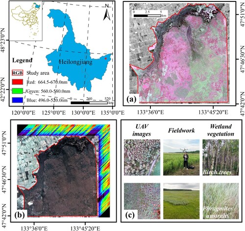
The Honghe National Nature Reserve (HNNR) (47°42′18″N-47°52′N, 133°34′38″E-133°46′29″E) is located at the junction of Tongjiang and Fuyuan Cities in the hinterland of the Sanjiang Plain in Heilongjiang Province, Northeast China (Figure 1). HNNR remains the entire original marsh scene of the Sanjiang Plain. As a large freshwater marsh, HNNR has high typicality and representativeness in the same bioclimatic zone of the world and was listed in the Ramsar Convention in 2002. HNNR has unique natural conditions, rich vegetation diversity, and a precious plant resource library with 175 families and 1005 species. Most vegetation types are herbaceous and aquatic marsh vegetation, such as Cyperaceae, Deyeuxia angustifolia swamp, and Phragmites australis. The climate of HNNR is temperate monsoonal with an average annual temperature of 1.9 °C. The rainfall is concentrated between July and September, and the freezing periods last from late September to mid-May. The vegetation diversity has brought out some challenges for finely classifying marsh vegetation using medium- and high-resolution images.

Figure 1. Geographical location of study area. (a) Sentinel-2A false-color composite images, (b) Zhuhai-1 hyperspectral false-color composite images, (c) The measured data of UAV and sample points.

2.2. Multi-source data acquisition

In this study, we selected four remote sensing images, including Gaofen-1 (GF-1), Sentinel-2A, Landsat 9 OLI (or Landsat 9 OLI-2), and Zhuhai-1 (OHS-02) from August 2021 and September 2022. The Sentinel-2A image was from the European Space Agency (ESA) (https://scihub.copernicus.eu/), carrying multispectral images covering 13 spectral bands with three spatial resolutions of 10, 20, and 60 m. The Landsat 9 OLI image was from the United States Geological Survey (USGS) (https://earthexplorer.usgs.gov/), with a Landsat 9 OLI sensor with nine spectral bands, including eight multispectral bands with 30 m spatial resolution, and a panchromatic band with 15 m spatial resolution. The GF-1 image was from China Centre for Resources Satellite Data and Application (http://www.cresda.com/CN/GF-1), a new generation of Chinese high-spatial-resolution remote sensing satellites. This study used four multispectral bands (blue, green, red, and near-infrared) and a panchromatic band with 60 km of the image width. The OHS-02 image was from Zhuhai Orbita Aerospace Technology Co China (https://www.obtdata.com/), a civil Orbita hyperspectral satellite constellation of China with four hyperspectral satellites (OHS-01, OHS-02, OHS-03, and OHS-04). We used the OHS-02 satellite carrying the CMOSMSS sensor, which covers 32 spectral bands with a spatial and spectral resolution of 10 m and 2.5 nm, respectively. The spectrum ranged from 400 to 1000 nm, and the imaging width was 150 km × 2500 km. Specific data sources which we uesd in this study are shown in Table 1.

Table 1. Parameters of multispectral and hyperspectral satellite images. NIR, near-infrared band, NNIR, narrow near infrared band, VRE, vegetation red edge band.

Sensors	Spectral bands	Wavelength ranges (nm)	Spatial resolution	Acquisition time	Sensors	Spectral bands	Wavelength ranges (nm)	Spatial resolution	Acquisition time
GF-1 PMS2	Blue	450–520	8 m	2021.09	Landsat 9 OLI	Coastal	433–453	30 m	2022.09
	Green	520–590				Blue	450–515
	Red	630–690				Green	525–600
	NIR	770–890				Red	630–680
	Pan	450–900	2 m			NIR	845–885
Sentinel-2A	Blue	458–523	10 m	2021.09		SWIR1	1560–1660
	Green	543–578				SWIR2	2100–2300
	Red	650–680				Pan	500–680	15 m
	NIR	785–900			OHS-02 CMOSMSS	Blue	466–500	10 m	2021.09
	NNIR	855–875	20 m			Green	520–596
	VRE1	698–713				Red	610–700
	VRE2	733–748				NIR	716–940
	VRE3	773–793
	SWIR1	1565–1655
	SWIR2	2100–2280

We used ENVI 5.6 software to implement the radiometric calibration and the atmospheric correction of GF-1, Landsat 9 OLI, and OHS-02 images. The atmospheric correction used the fast atmospheric correction (FLAASH) algorithm. The Gram-Schmidt (GS) method was used to fuse the multispectral and panchromatic bands from the GF-1 and Landsat 9 OLI images. The radiation correction of the Sentinel-2A images used the Sen2Cor processor in SNAP 8.0 software. The resampling using the S2 resampling processor tool resampled the spatial resolution of the 20 and 60 m bands to 10 m in Sentinel-2A. Using the band synthesis, we stitched and cropped images in the Python GDAL open-source tool.

3. Methods

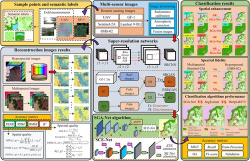
This study combined SR reconstruction and deep learning to classify marsh vegetation in the HNNR, northeast China using multispectral and hyperspectral images. The flowchart of this study was mainly composed of four parts (Figure 2): (1) collection and process of multi-sources remote sensing images, and creation of semantic labels by visual interpretation of unmanned aerial vehicle (UAV) image and field measurements; (2) reconstruction of multi-resolution multispectral and hyperspectral images using three SR networks, including SRCNN, SRGAN, and ESRGAN, and evaluation of their reconstructed image qualities of different marsh vegetation from spectral restoration and spatial resolution improvement; (3) design of an SGA-Net framework and verification of their marsh vegetation classification performance by comparing to the DeepLabV3 + and SegFormer algorithms; (4) evaluation of the accuracy improvement of marsh vegetation between original and reconstructed images to examine the feasibility of combing SR reconstruction with deep learning for classifying marsh vegetation.

Figure 2. Flowchart of classifying marsh vegetation using super-resolution reconstruction combined with SGA-Net algorithm.

3.1. Field measurements and semantic labels creation

The ground sampled data in this study was mainly derived from the visual interpretation of ultra-high resolution UAV images and sample data from the field measurements. We used the field measurements conducted between 24 and 30 August 2019 and 12 and 19 July 2021. A handheld high-precision real-time kinematic (RTK) recorded the geographic location of the 1 m × 1 m ground sampling points (horizontal accuracy of 0.25 m + 1 ppm). The UAV images were acquired by a DJI P4M with a multispectral sensor. We collected 47 aerial strips of the study area from 24–30 August 2019 and 12–19 July 2021 with the 30 m flight height. We determined vegetation types based on visual interpretation of the UAV digital orthophoto images (DOM) generated by Pix4Dmapper software, with a spatial resolution of 0.07 m and a projected coordinate system of WGS 1984 UTM Zone 49N.

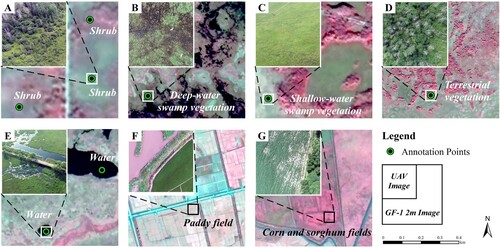
This study collected 1132 ground sample points, 852 points for marsh vegetation, including 233 points of shrub (e.g. S. Rosmarinifolia L.), 123 points of deep-water marsh vegetation (e.g. Carex pseudo-curaica), 213 points of shallow-water marsh vegetation (e.g. Deyeuxia angustifolia swamp), 283 points of terrestrial vegetation (e.g. Betula platyphylla forest), 92 points for water, 88 points for paddy field, and 100 points for corn and sorghum fields. The spaceborne remote sensing and UAV data are shown in Figure 3. The semantic labels of wetlands in this study were created based on the ultra-high spatial resolution UAV images and ground sample points. The specific definitions of marsh vegetation are presented in Appendix A.

Figure 3. The UAV and satellite multispectral images of different vegetation types in study area (A: shrub, B: deep-water marsh vegetation, C: shallow-water marsh vegetation, D: terrestrial vegetation, E: water, F: paddy field, G: corn and sorghum fields).

3.2. Super-resolution reconstruction

3.2.1. SRCNN

Figure 4 shows the architecture of the SR convolutional neural network (SRCNN) (Dong et al. 2016). The SRCNN constructed a three-layer convolutional network to directly learn the end-to-end mapping from low to high-resolution images. This study used the bicubic interpolation (BiCubic) method to increase the number of pixels in multispectral and hyperspectral remote sensing images (GF-1, Sentinel-2A, Landsat 9 OLI, and OHS-02) and inputted them to the SRCNN network. The reconstruction equation of the SRCNN network was defined as: (1) $\mathrm{BiCubic}(f_{H_{\mathrm{low}},W_{\mathrm{low}},C})=f_{3H,3W,C}$(1) (2) $f_{\mathrm{CNN}}=F_{\mathrm{SRCNN}}(f_{3H,3W,C})$(2) where $f_{H_{\mathrm{low}},W_{\mathrm{low}},C}$ is the training images for multispectral and hyperspectral, $H_{\mathrm{low}}$ and $W_{\mathrm{low}}$ are the height and width, and $C$ is the number of channels of image. $f_{\mathrm{CNN}}$ is the reconstruction image, and $F_{\mathrm{SRCNN}}$ represents the SRCNN network.

Figure 4. Structure of the super-resolution convolutional neural network (SRCNN).

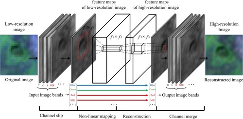
This study selected the mean squared error loss (MSELoss) function as the loss function of SRCNN, evaluating the perceived similarity between the original image and the corresponding points of the reconstructed image (Marmolin and Hans 1986). The calculation formula was defined as follows: (3) $L_{\mathrm{MSE}}={\displaystyle \frac{1}{m}\sum _{i=1}^m{(y_i-{\hat{y}}_t)}^2}$(3) where $L_{\mathrm{MSE}}$ denotes the MSELoss function, $y_i$ denotes the original image data, and ${\hat{y}}_i$ denotes the reconstructed image data.

3.2.2. SRGAN and ESRGAN

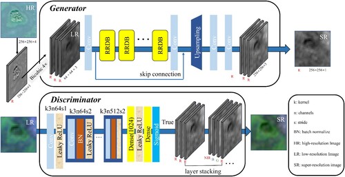
Figures 5 and 6 show the structure of the SR generative adversarial network (SRGAN) (Ledig et al. 2017) and the enhanced SR generative adversarial network (ESRGAN) (Wang et al. 2019), respectively. SRGAN and ESRGAN perform SR reconstruction of images using the generative adversarial network (GAN), consisting of the generator and the discriminator. This study used the BiCubic to reduce the number of pixels in the 2 m GF-1 images and input it to the generator. The reconstruction equation of the SRGAN and ESRGAN is defined as follows: (4) $\mathrm{BiCubic}(f_{H_{\mathrm{high}},W_{\mathrm{high}},C})=f_{{\displaystyle \frac{H}{4},{\displaystyle \frac{W}{4},C}}}$(4) (5) $f_{\mathrm{GAN}}=F_{\mathrm{SRGAN}}(f_{{\displaystyle \frac{H}{4},{\displaystyle \frac{W}{4},C}}})$(5) (6) $f_{\mathrm{GAN}}=F_{\mathrm{ESRGAN}}(f_{{\displaystyle \frac{H}{4},{\displaystyle \frac{W}{4},C}}})$(6) where $f_{H_{\mathrm{high}},W_{\mathrm{high}},C}$ is training data for the 2m GF-1 multispectral images, $C$ is the number of channels of image, $f_{\mathrm{GAN}}$ is the reconstructed image, $F_{\mathrm{SRGAN}}$ and $F_{\mathrm{ESRGAN}}$ represent the SRGAN and ESRGAN.

Figure 5. The structure of the super-resolution generative adversarial network (SRGAN).

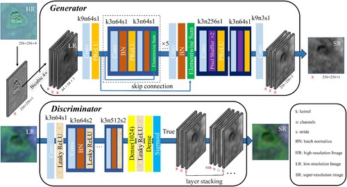
Figure 6. The structure of enhanced super-resolution generative adversarial network (ESRGAN).

The loss function of the GAN included the content loss function $l_X^{SR}$ and the adversarial loss function $l_{Gen}^{SR}$ (Ledig et al. 2017). In the SRGAN network, the content loss function was set to the MSELoss (3), and the adversarial loss function was set to mean absolute error (L1-Loss). The L1-Loss function was used to measure the average error magnitude between the reconstructed and the original image. The calculation formula was defined as follows: (7) $l_{}^{SR}=l_X^{SR}+{10}^{-3}{l}_{Gen}^{SR}$(7) (8) $L_{\mathrm{MAE}}={\displaystyle \frac{1}{m}\sum _{i=1}^m|y_i-{\hat{y}}_i|}$(8) where $L_{MAE}$ is the L1-loss function, and $l^{SR}$is the perceptual loss function.

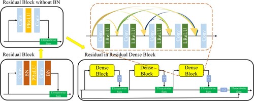
The ESRGAN introduces a residual-in-residual dense block (RRDB) to replace the residual block (RB) in the SRGAN network (Figure 7). In this paper, we selected the balanced cross-entropy (BCELoss) as the content loss function, and the L1-Loss as the adversarial loss function. The calculation formula is defined as: (9) $L_{\mathrm{BCE}}=-(y_i\log ({\hat{y}}_t)+(1-y_i)\log (1-{\hat{y}}_t))$(9) where $L_{\mathrm{BCE}}$ represents the BCELoss function.

Figure 7. The structure of the residual-in-residual dense block (RRDB) modules.

3.3. SGA-Net and SegFormer algorithms

3.3.1. SGA-Net algorithm

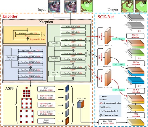
This study proposed a novel SGA-Net algorithm (Figure 8) and provided specific improvements in two aspects relative to the traditional encoder-decoder structure of the network, as follows: (1) we replaced the decoder with the SCE-Net, and introduced the Gaussian error linear units (GELU) in the backbone network (Xception) of the encoder, the atrous spatial pyramid pooling (ASPP), and the SCE-Net module. The GELU has the better performance in computer vision (Hendrycks and Gimpel 2016). In the encoder and the SCE-Net, the GN function was replaced with the batch normalization (BN) function, effectively avoiding performance degradation by setting batch size (Wu and He 2018). The number groups of the GN were set to the channels for half of the input image. In the SCE-Net module, we introduced the space and channel attention mechanism. The spatial attention mechanism chosen was the spatial transformer network (STN) (Jaderberg et al. 2015), and the channel attention mechanism was SK-Net (Li et al. 2019). The attention mechanism enabled the SCE-Net to focus more on processing the fact of contour details and spectral similarities between marsh vegetation. We added more low-level features in SCE-Net to enhance the segmentation performance, and increased the number of low-level features to 1/2, 1/4, and 1/8 sampling coefficients. The features are then refined with two 3 × 3 deep separable convolutions. The Adam optimizer was used for SGA-Net training, and the initial learning rate was set to 1 × 10^–4.

Figure 8. The structure of the SGA-Net algorithm proposed in this study. ASPP, atrous spatial pyramid pooling; GELU, Gaussian error linear unit; LR, low-resolution; SR, super-resolution; STN, spatial transformer network.

3.3.2. SegFormer algorithm

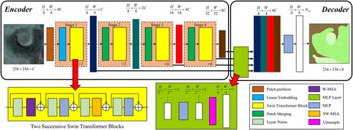
SegFormer algorithm, combined with transformer and visual classification, was developed by the Nvidia corporation and the University of Hong Kong in 2021. SegFormer algorithm is a simple, effective, and robust semantic segmentation method. SegFormer achieved an overview of state-of-the-art (SOTA) accuracy with good speed on classic semantic segmentation datasets and good performance in remote sensing image classifications (Deng et al. 2022). Figure 9 shows the structure of the SegFormer model (Xie et al. 2021), containing an encoding and a decoding layer. The encoder consisted of the four transformer blocks stacking. After processing each transformer block, the resolution of feature map became 1/4, 1/8, 1/16, and 1/32, respectively, and the four different resolution feature maps were fused in the decoder using the multilayer perceptron (MLP) layer. In this research, the window size was set to 12, the channel number of the hidden layers was set to 96, and layer numbers were {2, 2, 18, 2}. The Adam optimizer was set from 0.9 to 0.99, the weight decay was set to 2 × 10⁻⁵, and the initial learning rate was set to 1 × 10⁻⁴.

Figure 9. The structure of the SegFormer algorithm proposed in this study. MLP, multilayer perceptron; SW-MSA, shifted window multi-head self-attention; W-MSA, window multi-head self-attention.

3.3.3. Loss function

To resolve the class imbalance of marsh vegetation in the model training, this study selected the cross-entropy and DiceLoss (CE-DiceLoss) (Milletari, Navab, and Ahmadi 2016) as the loss function of SGA-Net and DeeplabV3 + algorithms, which has the stability of cross-entropy and the property of DiceLoss without being affected by class imbalance. The calculation formula was defined as follows: (10) $L_{\mathrm{Dice}}(y_i,y_i^{\mathrm{\prime }})={\displaystyle \frac{2^{\ast }|y_i\cap {y^{\mathrm{\prime }}}_i|+\mathrm{smooth}}{|y_i|+|{y^{\mathrm{\prime }}}_i|+\mathrm{smooth}}}$(10) (11) $L_{\mathrm{CE}}({\mathrm{y}}_i,y_i^{\mathrm{\prime }})=-\sum _{i=1}^m{y}_i\log p_{{y^{\mathrm{\prime }}}_i}$(11) (12) $L_{\mathrm{CE}+\mathrm{Dice}}={0.5}^{\ast }{L}_{\mathrm{CE}}+{0.5}^{\ast }{L}_{\mathrm{Dice}}$(12) where $y_i$ is the remote sensing image, $y_i^{\mathrm{\prime }}$ is the semantic label for deep learning, $\mathrm{smooth}$ is set to 1, and $p_{y_i^{\mathrm{\prime }}}$ represents the probability of predicted value.

3.4. Schemes of image reconstruction and marsh vegetation classification

3.4.1. Image reconstruction schemes

This study constructed fifty remote sensing image training datasets based on spectral single band, with two sets of image reconstruction strategies and 12 reconstruction schemes (Table 2). In schemes 1–4, the training and reconstruction were performed using the SRCNN model on a band-by-band basis for GF-1, Sentinel-2A, Landsat 9 OLI, and OHS-02 images. The specific band portfolio information is shown in Appendix B. From left to right, 50% of the image was used as the training image and 50–70% was used as the validation image. We cropped 50,000 images of 128 × 128 × 3 (H, W, C) size, respectively, including 80% of the data as training and 20% as verification. In schemes 4–12, the reconstruction of the GF-1, Sentinel-2A, Landsat 9 OLI, and OHS-02 images was performed using SRGAN and ESRGAN models trained on each of the four bands in the GF-1 fusion image (spatial resolution 2 m), including the blue (450–520 nm), green (520–590 nm), red (630–690 nm), and near-infrared (NIR) (770–890 nm) bands. The band-specific portfolio information is presented in Appendix B. We cropped 100,000 images of 256 × 256 × 3 size, respectively, including 80% of the data as training and 20% as verification.

Table 2. Twelve super-resolution reconstruction schemes for multispectral and hyperspectral images. SR networks: super-resolution networks; Numbers of bands: the bands of reconstructed images. SR, super-resolution; ESRGAN, enhanced super-resolution generative adversarial network; SRGAN, super-resolution generative adversarial network; SRCNN, super-resolution convolutional neural network.

SR networks	Schemes	Training sensors	Spatial resolution	Wavelength ranges (nm)	Reconstructed sensors	Spatial resolution	Wavelength ranges (nm)	Numbers of bands	Number of subimages
SRCNN	1	GF-1	8 m	450–890	GF-1	3 m	450–890	4	5 × 10^4
	2	Sentinel-2A	10 m	458–2280	Sentinel-2A	3.5 m	458–2280	9
	3	Landsat 9 OLI	15 m	430–2300	Landsat 9 OLI	5 m	430–2300	7
	4	OHS-02	10 m	400–1100	OHS-02	3.5 m	466–940	26
SRGAN	5	GF-1	2 m	450–890	GF-1	2 m	450–890	4	1 × 10^5
	6			450–890	Sentinel-2A	2.5 m	458–2280	9
	7			450–890	Landsat 9 OLI	3.75 m	430–2300	7
	8			450–890	OHS-02	2.5 m	466–940	26
ESRGAN	9	GF-1	2 m	450–890	GF-1	2 m	450–890	4	1 × 10^5
	10			450–890	Sentinel-2A	2.5 m	458–2280	9
	11			450–890	Landsat 9 OLI	3.75 m	430–2300	7
	12			450–890	OHS-02	2.5 m	466–940	26

As the SRGAN and ESRGAN models require high-resolution remote sensing images (GF-1 2m) to train the models, based on the image spatial resolution multipliers (images to be reconstructed: Sentinel-2A and OHS-02 are 10 m, and Landsat 9 OLI is 15 m), we selected 4× (increase in spatial resolution) reconstructions for both models. The SRCNN model was constructed based on the original images. Previous studies found that 3× ratio could achieve better quality of reconstructed images using the public dataset (Wang et al. 2021b; Ren, El-Khamy, and Lee 2017). Thus, this study selected 3× reconstructions for the SRCNN analysis. The spatial image resolution was resampled to the multiple of 0.5 when the spatial resolution had two decimal places.

3.4.2. Classification schemes of marsh vegetation

This study constructed 16 classification schemes of marsh vegetation based on classification algorithms and reconstructed images (Table 3). The training images for the SGA-Net, DeepLabV3+, and SegFormer algorithms were from the 12 SR reconstruction schemes, and the training label was from the semantic labels of wetlands. Using the left half of the study area as the training image and the other right half as the testing image, we trained the dataset of hundred thousand wetland images with the size of 256 × 256×C (C is the number of image bands), including 80% of the data as training and 20% as verification. We quantified the classification accuracy of marsh vegetation between original and reconstructed images by comparing schemes 1–12. By comparing schemes 13–16 with the same resolution, we quantified the classification accuracy of marsh vegetation in different spectral resolutions.

Table 3. Classification schemes of marsh vegetation derived from different images.

Algorithms	Schemes		Groups	Spatial resolution		SR methods	Spatial resolution	Sensors	Number of each scheme
SGA-Net, DeepLabV3+, SegFormer	1		Original images	8 m	VS	SRCNN	3 m	GF-1	1 × 10^5
	2			10 m			3.5 m	Sentinel-2A
	3			10 m			3.5 m	OHS-02
	4			15 m			5 m	Landsat 9 OLI
	5		Original images	8 m	VS	SRGAN	2 m	GF-1	1 × 10^5
	6			10 m			2.5 m	Sentinel-2A
	7			10 m			2.5 m	OHS-02
	8			15 m			3.75 m	Landsat 9 OLI
	9		Original images	8 m	VS	ESRGAN	2 m	GF-1	1 × 10^5
	10			10 m			2.5 m	Sentinel-2A
	11			10 m			2.5 m	OHS-02
	12			15 m			3.75 m	Landsat 9 OLI
Algorithms	Schemes	Sentinel-2A	Wavelength ranges (nm)	Numbers of bands		OHS-02	Wavelength ranges (nm)	Numbers of bands	Number of each scheme
SGA-Net, DeepLabV3+, SegFormer	13	Original	458–2280	9	VS	Original	466–940	26	1 × 10^5
	14	SRCNN			VS	SRCNN			1 × 10^5
	15	SRGAN			VS	SRGAN			1 × 10^5
	16	ESRGAN			VS	ESRGAN			1 × 10^5

3.5. Accuracy assessment

3.5.1. Evaluation indicators of image reconstruction

In this study, we quantitatively evaluated the reconstruction quality of multispectral and hyperspectral images using two main aspects: SAQ and SEQ. The spatial quality (SAQ) includes peak signal-to-noise ratio (PSNR) (Hore and Ziou 2010) and structural similarity (SSIM) metrics. The PSNR objectively assesses the difference in quality between the reconstructed and the original image. The SSIM measures the similarity between the reconstructed and the original image using three parameters: image brightness, contrast, and correlation. The PSNR was higher, and the SSIM was closer to 1, with better SAQ of the reconstructed image. The calculation formula was defined as follows: (13) $\mathrm{MSE}(f,g)={\displaystyle \frac{1}{MN}\sum _{i=1}^M\sum _{j=1}^N{(f_{ij}-g_{ij})}^2}$(13) (14) $\mathrm{PSNR}(f,g)={10}^{\ast }{\log }_{10}({\displaystyle \frac{{255.0}^2}{\mathrm{MSE}(f,g)})}$(14) (15) $\mathrm{SSIM}(f,g)=l(f,g)c(f,g)s(f,g)$(15) where $MN$ is the size of image, $f$ is the original image, $g$ is the reconstructed image, denotes the maximum value in image using 8-bit unint data type. $l(f,g)$ denotes the average spectral value of the image, $c(f,g)$ denotes the standard deviation spectral value of the image, $s(f,g)$ denotes the covariance spectral value of the image. The spectral quality (SEQ) includes RMSE and R² metrics for the spectral curve.

We extracted several pixel values from the reconstruction image based on the ground sample points, and then plotted the spectral curve, which was a 1:1 linear regression curve from the normalized spectral values between the original and reconstructed images. The x-axis is the original image spectral values, and the y-axis is the reconstructed image spectral values. The RMSE was smaller than 1, and the R² was closer to 1, with better SEQ of the reconstructed image. We standardized and normalized all image bands. The calculation formula was defined as follows: (16) $\mathrm{Std}(X)={\displaystyle \frac{x-X\mathrm{mean}}{X\mathrm{std}}}$(16) (17) $\mathrm{Norm}(X)={\displaystyle \frac{\mathrm{Std}(X)-X_{min}}{X_{max}-X_{min}}}$(17) (18) $\mathrm{RMSE}(f,g)=\sqrt{\mathrm{MSE}(f_{\mathrm{Std}+\mathrm{Norm}},g_{\mathrm{Std}+\mathrm{Norm}})}$(18) (19) $R(f,g{)}^2={\displaystyle \frac{\sum _{i=1}^M\sum _{j=1}^N{({\hat{f}}_{ij}-f_{ij})}^2}{\sum _{i=1}^M\sum _{j=1}^N{(g_{ij}-f_{ij})}^2}}$(19) where $x$ is the raw spectral value of vegetation, $X$ denotes the full spectral values in the image. $Norm(X)$ denotes the spectral value after normalization, $X_{\mathrm{std}}$ denotes the spectral value after standardization, $f$ denotes the original image data, $g$ denotes the reconstruction image data, and $\hat{f}$ denotes the estimation after bringing $f$ into the regression equation, the formula of $\mathrm{MSE}$ is in (13).

3.5.2. Accuracy assessment of classification results

This study used the accuracy evaluation metrics F1-score (Lipton, Elkan, and Naryanaswamy 2014), overall accuracy (OA), and mean intersection over union (MIoU) to quantitatively evaluate the classification accuracy of marsh vegetation. In F1-score and OA, the label data were obtained from the ground sample points data. In MIoU, the true label data were obtained from the semantic label for deep learning. First, we used the OA to compare the vegetation classification accuracy between SGA-Net, DeepLabV3+, and SegFormer algorithms. Then, we compared the classification accuracy of SGA-Net, DeepLabV3+, and SegFormer algorithms for marsh vegetation by F1-score. Finally, the F1-score and OA were calculated based on the ground sample point to verify that the classification result reflecting the overall trend of the image. We calculated the pixel-based MIoU. (20) $\mathrm{Precision}={\displaystyle \frac{X_{TP}}{X_{TP}+X_{FP}}}$(20) (21) $F1\text{-}\mathrm{score}={\displaystyle \frac{2\cdot \mathrm{Precision}\cdot \mathrm{Recall}}{\mathrm{Precision}+\mathrm{Recall}}}$(21) (22) $\mathrm{OA}={\displaystyle \frac{X_{TP}+X_{TN}}{X_{TP}+X_{FN}+X_{FP}+X_{TN}}}$(22) (23) $\mathrm{MIoU}={\displaystyle \frac{X_{TP}}{X_{FN}+X_{FP}-X_{TP}}}$(23) where $X_{TP}$ is the predicted vegetation types consistent with the labeling and the number of correct predictions, $X_{FP}$ is the predicted vegetation types inconsistent with the labeling and the number of correct predictions, $X_{TN}$ is the predicted vegetation types consistent with the labeling and the number of incorrect predictions, and $X_{FN}$ is the predicted vegetation types inconsistent with the labeling and the number of incorrect predictions.

4. Results and analysis

4.1. Quality assessment of reconstruction images

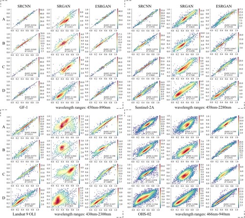
We compared the reconstruction results of the overall image using SRCNN, SRGAN, and ESRGAN and calculated the SAQ (PSNR & SSIM) and SEQ (RMSE & R²) (Table 4). (1) In SAQ, the higher PSNR value and the SSIM value closer to 1 indicate that the reconstruction image is more similar to the original image. The mPSNR ranged from 20.33 to 28.87, 18.15 to 23.32, and 19.17 to 27.68 for SRCNN, SRGAN, and ESRGAN, respectively, and the mSSIM ranged from 0.62 to 0.77, 0.38 to 0.51, and 0.46 to 0.79, respectively. In Figure 10 (o), the reconstruction results of SRGAN and ESRGAN appeared as noise (pixels), affecting the correctness of the vegetation edge information and causing the reduction of accuracy. In contrast, the ESRGAN reconstruction images (Figure 10 (p)) had less noise compared to SRGAN reconstruction images. The spatial reconstruction results of SRCNN and ESRGAN were better than those of SRGAN. (2) In SEQ, the closer RMSE value to 0 and the closer R² value to 1 indicate that the reconstructed image of spectral fidelity was greater. The RMSE ranged from 0.05 to 0.11, 0.09 to 0.26, and 0.07 to 0.15 for SRCNN, SRGAN, and ESRGAN, respectively, and R² were 0.63 to 0.95, 0.50 to 0.75, and 0.68 to 0.87, respectively. The spectra on the NIR reconstruction band on SRCNN-based (Figure 10 (f1)) and ESRGAN-based (Figure 10 (h1)) were generally consistent with the vegetation spectrum on the original image. However, the spectral on SRGAN-based differed (Figure 10 (g1)). In summary, the SRCNN and ESRGAN SR reconstruction methods were superior to the SRGAN regarding spectral fidelity and spatial detail enhancement.

Figure 10. Multispectral and hyperspectral super-resolution reconstruction images. (a)–(p): false color images, blue: 550–566 nm, green: 656–660 nm, red: 830–836 nm, (a1)–(p1): single band images of 830–836 nm (NIR). ESRGAN, enhanced super-resolution generative adversarial network; SRGAN, super-resolution generative adversarial network; SRCNN, super-resolution convolutional neural network.

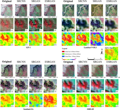
Table 4. The accuracies and score values of reconstruction images from different sensors. SEQ, spectral quality scores; SAQ, spatial quality scores; ESRGAN, enhanced super-resolution generative adversarial network; SRGAN, super-resolution generative adversarial network; SRCNN, super-resolution convolutional neural network. The mPSNR and mSSIM are the average PSNR and SSIM values of the reconstructed images cut into several 256 × 256 size images in a left-to-right and top-to-bottom order, and the RMSE and R² are the spectral values obtained from the ground sample points.

Sensors	SR networks	RMSE / SEQ	R² / SEQ	mPSNR / SAQ	mSSIM / SAQ
GF-1	SRCNN	0.05	0.95	27.61	0.77
	SRGAN	0.15	0.59	19.55	0.42
	ESRGAN	0.07	0.86	26.75	0.73
Sentinel-2A	SRCNN	0.11	0.90	27.43	0.74
	SRGAN	0.09	0.75	21.83	0.51
	ESRGAN	0.08	0.87	27.68	0.79
Landsat 9 OLI	SRCNN	0.07	0.87	20.33	0.62
	SRGAN	0.26	0.60	18.15	0.38
	ESRGAN	0.10	0.74	19.17	0.46
OHS-02	SRCNN	0.11	0.63	28.87	0.76
	SRGAN	0.13	0.50	23.32	0.47
	ESRGAN	0.15	0.68	26.68	0.72
	Ideal values/score	0	1	∞	1

4.1.1. Spatial enhancement of the reconstructed images for marsh vegetation

We quantitatively evaluated the spatial enhancement of the marsh vegetation and other feature types using three SR methods with four remote sensing sensors. For all the land cover types (Table 5), the mPSNR values were ranged from 8.31 to 31.02, the mSSIM values were ranged from 0.27 to 0.91. The mPSNR and mSSIM values decreased with the improvement of spatial resolutions of the reconstructed images, and no obvious differences of SAQ (PSNR and SSIM) in the same sensors by different reconstructed networks were observed. The reconstructed image of shrub using the Sentinel-2A sensor had the highest PSNR (30.57), and the reconstructed image of deep-water and shallow-water marsh vegetation and terrestrial vegetation using the OHS-02 sensor had the highest PSNR with 31.02, 29.07, and 28.46. For the marsh vegetation, the Landsat 9 OLI reconstructed images with the lowest mPSNR and mSSIM for deep-water marsh vegetation (20.82 and 0.49) and shallow-water marsh vegetation (22.01 and 0.53), the OHS-02 reconstructed images with the highest mPSNR and mSSIM in deep-water marsh vegetation (27.42 and 0.69), and shallow-water marsh vegetation (26.07 and 0.63). Therefore, the high spectral resolution of hyperspectral images relative to multispectral images positively affected the reconstruction of marsh vegetation.

Table 5. The accuracies of reconstruction images from different vegetations types using four remote sensing sensors. Drawing the 128 × 128 size images with the sampling points as the center as the vegetation types. The bolded numbers indicate the mean of the three super-resolution reconstruction accuracy values (mPSNR and mSSIM) for the marsh vegetation. ESRGAN, enhanced super-resolution generative adversarial network; SRGAN, super-resolution generative adversarial network; SRCNN, super-resolution convolutional neural network.

Sensors	SR methods	(mPSNR | mSSIM)
		Shrub	Deep-water marsh vegetation	Shallow-water marsh vegetation	Terrestrial vegetation	Water	Paddy field	Corn and sorghum fields
GF-1 (8m)	SRCNN (3m)	25.47 | 0.73	30.48 | 0.83	27.61 | 0.78	26.88 | 0.74	28.38 | 0.81	13.99 | 0.65	28.45 | 0.81
	SRGAN (2m)	21.01 | 0.45	16.55 | 0.41	20.22 | 0.45	20.42 | 0.37	16.75 | 0.39	15.11 | 0.62	18.59 | 0.27
	ESGAN (2m)	25.72 | 0.72	29.03 | 0.79	26.76 | 0.76	25.50 | 0.67	26.19 | 0.74	20.96 | 0.91	23.71 | 0.73
Mean:		24.07 | 0.63	25.64 | 0.67	24.86 | 0.66	24.27 | 0.59	23.77 | 0.65	16.69 | 0.73	23.58 | 0.60
Sentinel-2A (10m)	SRCNN (3.5m)	28.75 | 0.75	24.79 | 0.72	29.42 | 0.78	26.77 | 0.71	23.94 | 0.73	14.92 | 0.64	30.14 | 0.84
	SRGAN (2.5m)	23.44 | 0.57	19.45 | 0.41	22.25 | 0.54	22.19 | 0.53	19.00 | 0.45	16.90 | 0.61	23.81 | 0.47
	ESGAN (2.5m)	30.57 | 0.88	22.51 | 0.64	29.43 | 0.78	28.21 | 0.85	23.51 | 0.65	21.42 | 0.67	29.52 | 0.83
Mean:		27.59 | 0.73	22.25 | 0.59	27.03 | 0.70	25.72 | 0.70	22.15 | 0.61	17.75 | 0.64	27.82 | 0.71
Landsat 9 OLI (15m)	SRCNN (5m)	14.05 | 0.53	22.09 | 0.62	24.07 | 0.69	21.13 | 0.63	23.63 | 0.79	21.44 | 0.51	23.07 | 0.78
	SRGAN (3.75m)	14.15 | 0.44	19.20 | 0.37	20.21 | 0.40	19.05 | 0.31	17.81 | 0.39	21.81 | 0.28	18.94 | 0.29
	ESGAN (3.75m)	15.32 | 0.42	21.18 | 0.47	21.76 | 0.52	18.41 | 0.45	22.20 | 0.60	19.71 | 0.43	22.85 | 0.69
Mean:		14.51 | 0.46	20.82 | 0.49	22.01 | 0.53	19.53 | 0.46	21.21 | 0.59	20.99 | 0.41	21.62 | 0.59
OHS-02 (10m)	SRCNN (3.5m)	26.94 | 0.72	31.02 | 0.81	29.07 | 0.75	28.46 | 0.77	30.73 | 0.84	20.41 | 0.66	30.28 | 0.82
	SRGAN (2.5m)	21.78 | 0.44	23.02 | 0.50	23.82 | 0.45	24.67 | 0.50	21.41 | 0.49	25.41 | 0.79	27.05 | 0.75
	ESGAN (2.5m)	25.72 | 0.67	28.22 | 0.78	25.38 | 0.70	27.42 | 0.72	27.67 | 0.80	21.65 | 0.88	8.31 | 0.52
Mean:		24.81 | 0.61	27.42 | 0.69	26.07 | 0.63	26.85 | 0.66	26.60 | 0.71	22.49 | 0.78	21.88 | 0.70

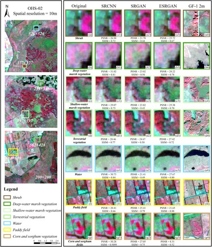
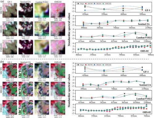
Figure 11 shows the spatial texture information of the marsh vegetation and other feature types in OHS-02 reconstructed images with their SAQ. The SRCNN outperformed SRGAN and ESRGAN for reconstructing images of deep-water and shallow-water marsh vegetation. In the SRCNN-based reconstructed images, deep-water marsh vegetation and water exhibited the highest PSNR and SSIM values of 31.02 and 0.84, respectively. The deep-water marsh vegetation and its surrounding scenes showed better boundary definition and color differences closer to the original image (Figure 11 (b1)). In the SRGAN-based reconstructed images, corn and sorghum, and paddy fields had the highest PSNR (27.05) and SSIM (0.79), respectively. In the ESRGAN-based reconstructed images, deep-water marsh vegetation and paddy field had the highest PSNR (28.22) and SSIM (0.88), respectively. Therefore, the accuracy of SRCNN and ESRGAN was better than that of SRGAN in comparing the SAQ of the marsh vegetation reconstruction results. The Landsat 9 OLI reconstruction image results are shown in Appendix C.

Figure 11. The spatial quality of the reconstructing OHS-02 images in different vegetation types. PSNR, peak signal-to-noise ratio; SSIM, structural similarity; ESRGAN, enhanced super-resolution generative adversarial network; SRGAN, super-resolution generative adversarial network; SRCNN, super-resolution convolutional neural network.

4.1.2. Spectral fidelity of the reconstructed images for marsh vegetation

We quantitatively evaluated the spatial fidelity of the wetland vegetation (shrub, deep-water marsh vegetation, shallow-water marsh vegetation, and terrestrial vegetation) in remote sensing sensors. Using the ground sample points to extract the spectral values on each image band, we calculated the degree of fit between the reconstructed spectral values of the wetland vegetation and the original spectral values and analyzed the reconstruction results of the SR network in different wavelength ranges. Figure 12 shows the density distribution of the wetland vegetation spectral values. We found that in deep-water marsh vegetation, the Landsat 9 OLI reconstructed image based on ESRGAN had the lowest RMSE and R². In contrast, the OHS-02 reconstructed image based on the ESRGAN network obtained the highest RMSE (0.05) and R² (0.93) values, respectively. In the shallow-water marsh vegetation, the GF-1 reconstruction images based on the SRGAN network produced the lowest RMSE and R², while their ESRGAN-based reconstructed images provided the highest RMSE (0.03) and R² (0.97), respectively. The SR reconstruction algorithms used in this study could achieve band-by-band spectral fidelity on both multispectral and hyperspectral images. However, the spectral quality (RMSE and R²) of OHS-02 (hyperspectral image) for marsh vegetation was lower than that of Sentinel-2A (multispectral image) in most reconstruction schemes.

Figure 12. Quantitative evaluation of the consistency of reconstructed and original spectra values in the marsh scenes using different sensors. A: shrub, B: deep-water marsh vegetation, C: shallow-water marsh vegetation, D: terrestrial vegetation. The total number of sample points: GF-1, 4,500; Sentinel-2A, 10,125; Landsat 9 OLI, 6,810; and OHS-02, 22,230. The color closer to red indicates the higher density distribution, and closer to blue indicates the sparse density distribution. ESRGAN, enhanced super-resolution generative adversarial network; SRGAN, super-resolution generative adversarial network; SRCNN, super-resolution convolutional neural network.

Therefore, we analyzed the changes in spectral values of deep-water marsh vegetation (Figure 13(a)) and shallow-water marsh vegetation (Figure 13 (b)) in the spectral range of the reconstructed images. For GF-1 images, the reconstructed results of the marsh vegetation were close to the original image values in the wavelength range around 550 and 890 nm, while there were significant differences in the wavelength range around 450 and 660 nm. For Sentinel-2A and Landsat 9 OLI images, the spectral differences of marsh vegetation were mainly concentrated between 660 and 865 nm, among which, the spectral values of the three reconstructed images were consistent but different from the original spectral values near 865 nm for Landsat 9 OLI. For OHS-02 images, the smaller magnitude of deviation exists in the 610–940 nm wavelength interval, and although the errors on individual bands were lower than those on individual bands of the multispectral images, their cumulative errors were higher, which result in lower spectral quality of the reconstructed images. The specific band differences were in Appendix D.

Figure 13. The relationship between the spatial resolution improvement and reconstructed spectral values for deep-water and shallow-water marsh vegetation. PSNR, peak signal-to-noise ratio; SSIM, structural similarity; ESRGAN, enhanced super-resolution generative adversarial network; SRGAN, super-resolution generative adversarial network; SRCNN, super-resolution convolutional neural network.

4.2. Comparison of classification results between different reconstruction images

We compared and analyzed the classification accuracies (OA, F1-score and MIoU) of multispectral and hyperspectral images using the SGA-Net, DeepLabV3 + and SegFormer algorithms in Table 6. We found that the reconstruction images both produced the better classification results than the original images. For example, the F1-score of Sentinel-2A reconstruction images increased from 0.28% to 13.96% compared to the original images, and OHS-02 reconstruction images increased from 3.3% to 15.08%. For hyperspectral reconstruction images, the classification accuracies derived from ESRGAN-based reconstruction images (78.08–81.64%) were mostly higher than that based on SRCNN (72.58–79.81%) and SRGAN (75.03–80.64%). (1) For the perspective of visual interpretation, the accuracy of edge profile information at the junction of shrub and deep-water marsh vegetation in SRCNN and ESRGAN reconstructed images was better than that in SRGAN reconstructed images, such as Figure 14 (k1), Figure 14 (k2) and Figure 14 (k3). The spatial integrity of shrub and shallow-marsh vegetation in the ESRGAN reconstructed images was better than in the SRCNN reconstructed images, such as Figure 14 (j1 and j3). (2) For the classification algorithms, the F1-score classification accuracy of the reconstructed images based on the SGA-Net algorithm ranged from 75.09% to 87.71%, the F1-score classification accuracy of the reconstructed images based on the DeepLabV3 + algorithm ranged from 72.04% to 86.58%, and the F1-score classification accuracy of the reconstructed images based on the Segformer algorithm ranged from 79.81% to 87.16%. The classification accuracy of Landsat 9 OLI reconstructed images was the lowest and that of GF-1 reconstructed images was the highest. Therefore, the SR-based reconstructed multi-hyperspectral and hyperspectral images were able to improve the classification accuracy of wetland images, in which the ESRGAN network outperformed SRCNN and SRGAN networks in the classification results, and the SGA-Net algorithm achieved the higher classification accuracies than DeepLabV3 + and SegFormer algorithms in most classification schemes.

Figure 14. Classification results of SGA-Net, DeepLabV3+, and SegFormer algorithms with multispectral and hyperspectral reconstruction images. ESRGAN, enhanced super-resolution generative adversarial network; SRGAN, super-resolution generative adversarial network; SRCNN, super-resolution convolutional neural network.

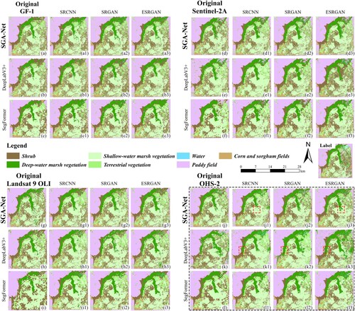
Table 6. Classification accuracies of reconstructed images with different sensors based on SGA-Net, DeepLabV3 and SegFormer algorithms. The *value indicates the highest classification accuracy value of the image, and the value* indicates the highest classification accuracy value of the image. MIoU, mean intersection over union; OA, overall accuracy; ESRGAN, enhanced super-resolution generative adversarial network; SRGAN, super-resolution generative adversarial network; SRCNN, super-resolution convolutional neural network.

SR networks	Accuracies	Sensors	SGA-Net (Ours) (%)	DeepLabV3+ (%)	SegFormer (%)	Sensors	SGA-Net (Ours) (%)	DeepLabV3+ (%)	SegFormer (%)
Original	OA	GF-1	84.36	84.21	83.86	Sentinel-2A	80.02	79.41	67.36*
	F1		83.62	84.33	84.64		78.99	80.75	68.31*
	MIoU		74.10	68.99	66.84		69.59	61.52	59.11*
SRCNN	OA		87.50	81.36*	84.91		82.54	80.66	81.52
	F1		87.71	82.72*	85.39		83.60	81.03	82.27
	MIoU		66.22	62.06*	75.87		70.40	64.03	73.14
SRGAN	OA		86.43	85.96	86.90		84.55	82.66	80.58
	F1		86.89	86.50	87.16		*85.37	83.83	81.19
	MIoU		78.80	70.89	78.57		80.79	70.04	73.89
ESRGAN	OA		*87.97	85.84	86.08		*84.66	82.42	80.70
	F1		*88.46	86.58	86.34		85.28	83.17	81.33
	MIoU		*80.67	71.58	78.27		*82.02	67.62	78.22
Original	OA	Landsat 9 OLI	76.02	62.33	52.98*	OHS-02	73.45	62.22*	70.06
	F1		76.57	72.80	53.66*		74.03	63.75*	70.74
	MIoU		57.71	53.98	41.01*		59.35	48.22*	57.75
SRCNN	OA		74.61	71.11	79.65		76.84	72.16	79.88
	F1		75.09	72.04	80.11		77.33	72.58	79.81
	MIoU		58.78	53.29	65.22		63.68	60.65	*70.32
SRGAN	OA		78.47	76.49	82.57		77.94	74.15	81.05
	F1		79.43	76.46	83.06		78.55	75.03	80.64
	MIoU		67.02	57.90	*74.31		62.99	55.79	69.66
ESRGAN	OA		*82.92	79.41	80.00		77.78	78.48	*81.64
	F1		*83.12	79.92	80.41		78.08	78.83	*81.64
	MIoU		71.95	61.36	69.16		65.54	55.71	69.95

4.2.1. Classification results of different spatial-resolution sensors

We quantitatively compared and analyzed the effect of different spatial resolution on the wetland vegetation (shrub, deep-water marsh vegetation, shallow-water marsh vegetation and terrestrial vegetation) classification using Sentinel-2A (10 m spatial resolution) and Landsat 9 OLI multispectral images (15 m spatial resolution). The classification results of the reconstructed images were presented in Appendix E. Table 7 displayed the classification accuracies, including F1-score and MIoU, for the four vegetation types. The F1-scores ranged from 66.94–84.28% using the SGA-Net algorithm, and ranged from 59.59–82.41% using DeepLabV3 + algorithm, and ranged from 53.39–80.86% using SegFormer algorithm. The reconstructed images achieved the higher classification accuracies for all vegetation types than the original images. With the improvement of F1-score and MIoU of marsh vegetation from original images to reconstructed images, the F1-score of Sentinel-2A (10–2.5 m) increased in the range of 0–11.90%. The F1-score of deep-water marsh vegetation based on ESRGAN raised the most, and the F1-score of shallow-water marsh vegetation based on SRCNN raised the most, in which it could be seen that the water was correctly classified and the misclassification of deep-water marsh vegetation and shallow-water marsh vegetation was also corrected. The improvement in F1-score for Landsat 9 OLI (5–3.75 m) ranged from 0–24.62%. The largest improvement in F1-score of deep-water marsh vegetation and shallow-water marsh vegetation both based on SRGAN.

Table 7. The classification accuracies of marsh vegetations with different spatial resolutions. The *value indicates the highest classification accuracy value of the F1-score. MIoU, mean intersection over union; ESRGAN, enhanced super-resolution generative adversarial network; SRGAN, super-resolution generative adversarial network; SRCNN, super-resolution convolutional neural network.

		Sentinel-2A (%)				Landsat 9 OLI (%)
		Original	SRCNN	SRGAN	ESRGAN	Original	SRCNN	SRGAN	ESRGAN
		SGA-Net
Shrub	F1	75.06	74.31	*80.92	78.53	64.49	66.00	72.32	76.84
	MIoU	61.72	63.48	75.95	77.49	47.45	51.28	60.62	63.92
Deep-water marsh vegetation	F1	69.40	73.97	*74.17	72.64	66.94	73.77	72.00	72.81
	MIoU	85.97	89.76	91.88	93.36	73.92	83.45	86.10	86.96
Shallow-water marsh vegetation	F1	82.85	81.73	82.13	*84.28	75.00	73.21	74.67	80.18
	MIoU	73.17	75.33	84.18	85.41	63.21	64.07	72.73	75.96
Terrestrial Vegetation	F1	92.42	94.70	94.85	*95.32	89.36	82.88	90.30	93.33
	MIoU	57.49	53.05	71.16	71.83	46.26	36.34	48.65	60.98
		DeepLabV3+
Shrub	F1	71.84	68.65	*78.19	76.03	60.91	63.38	64.98	71.24
	MIoU	50.82	54.42	63.02	59.27	45.92	43.84	51.86	52.74
Deep-water marsh vegetation	F1	68.47	*75.74	75.67	73.24	59.59	70.63	67.27	68.72
	MIoU	77.65	81.74	83.44	79.95	66.24	76.46	69.05	77.05
Shallow-water marsh vegetation	F1	79.91	78.61	*82.41	79.59	71.93	69.18	74.47	78.66
	MIoU	66.04	70.65	70.56	68.11	63.28	59.79	64.32	66.56
Terrestrial Vegetation	F1	91.99	92.83	91.66	*94.15	86.39	80.26	76.49	90.87
	MIoU	51.58	49.30	63.14	63.16	40.47	33.09	46.37	49.10
		SegFormer
Shrub	F1	54.23	74.27	72.68	74.45	44.91	75.40	75.63	*76.88
	MIoU	52.93	68.95	69.07	74.40	34.62	59.70	69.86	65.05
Deep-water marsh vegetation	F1	60.51	70.22	69.81	72.41	53.39	75.21	*78.01	75.63
	MIoU	76.27	91.76	89.28	93.30	52.86	87.81	92.51	91.47
Shallow-water marsh vegetation	F1	71.57	79.91	79.63	77.27	60.59	76.39	*80.86	75.48
	MIoU	67.40	78.42	79.60	83.18	54.46	70.73	79.72	73.64
Terrestrial Vegetation	F1	78.35	*93.87	92.31	92.14	54.70	87.68	91.45	88.01
	MIoU	39.86	53.42	57.60	62.00	22.10	42.63	55.15	46.49

4.2.2. Classification results of different spectral band images

We further quantitatively analyzed the effect of increasing spectral resolution using Sentinel-2A multispectral image and OHS-02 hyperspectral image (Table 8). The classification results of the reconstructed images were presented in Appendix E. The classification accuracy of the OHS-02 (460–940 nm) original images was lower than the Sentinel-2A (458–2280 nm) original images using the SGA-Net and DeepLabV3 + algorithms with the difference in F1-score ranging from 0–10.47%. The super-resolution network improved F1-score from 0–14.77% based on OHS-02 images, which was higher than Sentinel-2A (0–11.90%). The classification results of Sentinel-2A and OHS-02 reconstructed images both regularly appeared the misclassification of marsh vegetation and shrub, which resulted in the classification accuracy of marsh vegetation and shrub lower than terrestrial vegetation. The MIoU accuracy improvement for the reconstructed Sentinel-2A (458–2280 nm) images ranged from 2.3% to 17.03%. The MIoU accuracy improvement for the reconstructed OHS-02 (460–940 nm) images ranged from 0.48–19.32%. Therefore, in this study, there was not significant differences of classification accuracies between the reconstructed hyperspectral images (OHS-02) and multispectral images (Sentinel-2A) under the same spatial resolution.

Table 8. The classification accuracies of marsh vegetations with different spectral ranges. The *value indicates the highest classification accuracy value of the F1-score. MIoU, mean intersection over union; OA, overall accuracy; ESRGAN, enhanced super-resolution generative adversarial network; SRGAN, super-resolution generative adversarial network; SRCNN, super-resolution convolutional neural network.

		Sentinel-2A				OHS-02
		Original	SRCNN	SRGAN	ESRGAN	Original	SRCNN	SRGAN	ESRGAN
		SGA-Net
Shrub	F1	75.06	74.31	*80.92	78.53	64.69	71.42	68.63	67.94
	MIoU	61.72	63.48	75.95	77.49	52.72	57.32	56.89	59.19
Deep-water marsh vegetation	F1	69.40	73.97	74.17	72.64	66.97	72.88	*75.92	71.55
	MIoU	85.97	89.76	91.88	93.36	82.64	87.31	83.12	86.49
Shallow-water marsh vegetation	F1	82.85	81.73	82.13	*84.28	75.05	73.74	78.47	75.84
	MIoU	73.17	75.33	84.18	85.41	65.94	69.19	68.36	71.23
Terrestrial Vegetation	F1	92.42	94.70	94.85	*95.32	82.22	85.43	86.11	88.85
	MIoU	57.49	53.05	71.16	71.83	36.09	40.91	43.58	45.24
		DeepLabV3+
Shrub	F1	71.84	68.65	*78.19	76.03	51.95	60.89	61.03	72.18
	MIoU	50.82	54.42	63.02	59.27	38.97	54.06	43.43	50.10
Deep-water marsh vegetation	F1	68.47	*75.74	75.67	73.24	57.64	68.52	72.41	69.12
	MIoU	77.65	81.74	83.44	79.95	68.97	83.14	73.47	69.97
Shallow-water marsh vegetation	F1	79.91	78.61	*82.41	79.59	64.46	67.91	72.84	76.66
	MIoU	66.04	70.65	70.56	68.11	55.57	67.08	62.86	65.02
Terrestrial Vegetation	F1	91.99	92.83	91.66	*94.15	73.40	85.07	86.76	88.49
	MIoU	51.58	49.30	63.14	63.16	29.39	38.34	43.39	37.75
		SegFormer
Shrub	F1	54.23	74.27	72.68	*74.45	60.49	72.83	71.30	72.57
	MIoU	52.93	68.95	69.07	74.40	52.65	65.91	63.89	64.78
Deep-water marsh vegetation	F1	60.51	70.22	69.81	72.41	64.45	70.25	72.73	*74.17
	MIoU	76.27	91.76	89.28	93.30	71.03	90.57	90.35	89.87
Shallow-water marsh vegetation	F1	71.57	*79.91	79.63	77.27	75.05	73.74	78.47	75.84
	MIoU	67.40	78.42	79.60	83.18	68.83	75.87	75.59	75.78
Terrestrial Vegetation	F1	78.35	*93.87	92.31	92.14	80.14	89.48	89.95	91.24
	MIoU	39.86	53.42	57.60	62.00	38.50	48.95	48.80	49.39

4.3. Evaluation of classification performances of SGA-Net algorithm

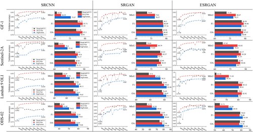
Figure 15 displayed the validation accuracy of the SGA-Net, DeepLabV3 + and SegFormer models at the first fifteen iterations. The SGA-Net algorithm obtained the highest validation accuracy (0.813–0.967) using the reconstructed images, followed by DeepLabV3+ (0.574–0.963) and SegFormer (0.692–0.894). The validation accuracy of SGA-Net presented a stable rising trend. In the GF-1 images, the accuracy metrics of the SGA-Net and SegFormer algorithms were higher than DeepLabV3 + algorithm, and the SRCNN-based reconstructed images using the SGA-Net algorithm achieved the highest accuracies in the OA and F1-score. Meanwhile, our algorithm achieved the higher accuracy metrics than the other two deep learning using the Sentinel-2A images. For the Landsat 9 OLI images, the SegFormer algorithm provided the highest accuracy metrics for reconstructed images based on SRCNN and SRGAN networks, and the SGA-Net algorithm was the highest accuracy metric for reconstructed images based on ESRGAN networks. For the OHS-02 images, the SegFormer algorithm obtained the highest accuracy metrics. The accuracy metrics of the GF-1 reconstructed images (spatial resolution: 2–3 m) was higher than the Sentinel-2A (spatial resolution: 2.5–3.5 m), OHS-02 (spatial resolution: 2.5–3.5 m) and Landsat 9 OLI (spatial resolution: 3.75–5 m) reconstructed images. More details of the model training were given in Appendix F.

Figure 15. Differences in the validation accuracy and accuracy metrics between SGA-Net, DeepLabV3+, and SegFormer. ESRGAN, enhanced super-resolution generative adversarial network; SRGAN, super-resolution generative adversarial network; SRCNN, super-resolution convolutional neural network.

5. Discussion

5.1. Difference analysis of the reconstructed spectral values of marsh vegetation

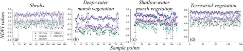
This study used SR reconstruction techniques based on CNN and GAN to reconstruct hyperspectral remote sensing images in the HNNR of northeast China. The multispectral and hyperspectral reconstructed results based on the SRCNN and ESRGAN networks were better than that of SRGAN under spatial and spectral quality criteria (Table 3). In contrast, granular noise appeared in SRGAN and ESRGAN reconstructed images, which is similar to previous studies (Ma et al. 2020), decreasing the SAQ of the image (PSNR and SSIM) as the number of noise points in the reconstructed image increased. Particularly, the reconstructed spectral values of some wetland vegetation significantly differ from that of the original images. Generally, the Near Infrared (NIR) bands have a high potential for identifying moisture content from soil and plant, and have confirmed to be useful in identifying wetland vegetation types (Nasser Mohamed Eid et al. 2020). Therefore, we calculated the normalized differential vegetation index (NDVI) using the original and reconstructed hyperspectral images (Figure 16 and Appendix G), respectively, analyzed the difference of the NDVI values of four marsh vegetations between the reconstructed and original images, and further revealed the reason for ESRGAN-based reconstructed images with the higher classification accuracy than that of SRCNN reconstructed images. (24) $NDVI={\displaystyle \frac{NI{R}_{836\mathrm{nm}}-R_{656\mathrm{nm}}}{NI{R}_{836\mathrm{nm}}+R_{656\mathrm{nm}}}}$(24)

We found that the NDVI values of the SRCNN reconstructed images fitted better with the original images. In contrast, the NDVI values of the SRGAN and ESRGAN reconstructed images were closer to the training images (GF-1, 2 m). Although the SRCNN improves the spatial resolution of the reconstructed hyperspectral images, the spatial heterogeneity of different vegetation patches is reduced (Zhong et al. 2016), and the spectral similarity of vegetation canopy is increased, resulting in the reconstructed images gradually failed to distinguish the difference of vegetations types in the real wetland scenes. These conclusions clarify the reasons for the SRCNN reconstructed images with the good spatial and spectral quality, and without achieving high classification accuracy of marsh vegetations. In contrast, the reconstructed images based on SRGAN and ESRGAN present a better spectral separability of marsh vegetations, because the high spatial resolution training images (GF-1, 2 m) is able to differentiate the spectral features of vegetation types (Figure 16). These results could explain the reasons for the GAN-based network of semantic segmentation producing a good classification performance in marsh scene.

Figure 16. The NDVI values of four wetland vegetation based on the reconstructed and training images.

5.2. Advantages and disadvantages for deep learning algorithms for marsh vegetation mapping

We further explored the combination of SR reconstruction methods and semantic segmentation algorithms for vegetation classifications in marsh scenes (Figure 17), and analyzed their performance for classifying marsh vegetation types. We found that accuracy improvements of the reconstructed image were small compared to the original GF-1 images. The Landsat 9 OLI reconstructed images displayed the largest accuracy improvements compared to the original images, with the largest improvement of 24.62% (F1-score) based on the SegFormer algorithm (Figure 17 (k)). However, its highest classification accuracy for marsh vegetation was lower than that of Sentinel-2A and OHS-02 reconstructed images. The SRGAN and ESRGAN models based on the fused GF-1 images (2 m) showed limited accuracy improvement compared to the original GF-1 images (8 m). In contrast, the most significant improvement in classification accuracy after image reconstruction was observed for the Landsat 9 OLI images (15 m) with the largest difference in spatial resolution. Some previous studies have also demonstrated the imaging fusion could improve the classification accuracy of single remote sensing sensor (Fu et al. 2017). However, the spectral information of the fusion images may present a certain extent of bias when the spatial resolution between the fused and original images exists great difference (Ghimire, Lei, and Juan 2020), and the classification improvement were also be limited (Fu et al. 2022). Taking advantage of imaging fusion and super-resolution reconstruction techniques may be an ideal method to improve the classification accuracy of vegetation types in marsh scenes using the coarse spatial resolution images.

Figure 17. Comparison of F1-score of different vegetation using SGA-Net with multispectral constructed images. A: shrub, B: deep-water marsh vegetation, C: shallow-water marsh vegetation, D: terrestrial vegetation. ESRGAN, enhanced super-resolution generative adversarial network; SRGAN, super-resolution generative adversarial network; SRCNN, super-resolution convolutional neural network.

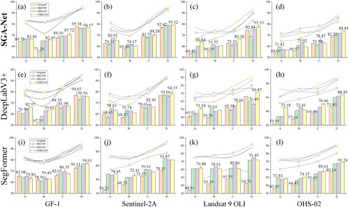
The SGA-Net algorithm could not fully achieve better classification results based on the OHS-02 hyperspectral reconstructed images compared to the other two deep learning models. The highest classification accuracy of SGA-Net (GF-1: 87.72%, Sentinel-2A: 84.28%, Landsat 9 OLI: 80.18%, and OHS-02: 78.47%) and SegFormer (86.35%, 79.91%, 80.86%, 76.66% and 80.61%) algorithms for marsh vegetation using multispectral and hyperspectral images was higher than that of DeepLabV3 + algorithm (84.39%, 82.41%, 78.66% and 76.66%) (Figure 17). There was a strong spatial competition relationship between shrub and wetland vegetation in wetland environments (Magnússon et al. 2021), resulting in the difficulty for distinguishing between each other. However, in this paper, the SGA-Net algorithm achieved better identification ability of shrub (SGA-Net, 64.69 & SegFormer, 60.49 in OHS-02) and marsh vegetation (the mean of deep- and shallow-water marsh vegetation) (SGA-Net, 70.35 & SegFormer, 67.45 in OHS-02) using the original four sensor images compared to the SegFormer model. Besides, the SGA-Net algorithm also achieved better identification ability of shrub and marsh vegetation using the original and reconstructed images compared to DeepLabV3 + model. The above results demonstrated the SGA-Net algorithm present better stability and performance than DeepLabV3 + and SegFormer algorithms for marsh vegetation classification.

5.3. Demonstration of SCE-Net module for marsh vegetation mapping

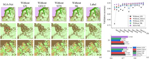
We used the OHS-02 original images as training and testing data to validate the classification contributions of the SCE-Net module (GN and GELU functions, STN and SK Attentions) in the SGA-Net model, respectively. We found that GN and GELU functions could make the model fit faster, and improve the F1-score of hyperspectral images from 0.0282 to 0.0356. Besides, the STN attention and SK attention could significantly improve the F1-score of hyperspectral images from 0.0552 to 0.0625, identify the small vegetation patch and fine delineate the boundary of different marsh vegetations. These results demonstrate the SGA-Net model with the integration SCE-Net module in this paper is effective for marsh vegetation mapping.

5.4. Limitations

Our works still have several limitations, including (1) the spectral range of GF-1 multispectral images was 450–890 nm, which could not cover the spectral range of Sentinel-2A (443–2190 nm) and OHS-02 (466–940 nm) completely, and may lead to the reconstructing images with the spectral uncertainty in the range of 890–2190 nm. Besides, the spectral quality of the sensitive bands (such as red edge) to marsh vegetation may cause the misclassifications; (2) in the SCE-Net module, we found that the channel attention mechanism (SK-Net) and spatial attention mechanism (STN-Net) could effectively improve the classification accuracy of marsh vegetation (Figure 18), however, there were still limitations in distinguishing between shrub and marsh vegetation, the GN function could perform the SGA-Net model fitting faster, but it could not produce the significant improvement in classification accuracy; (3) our study achieved the good performance in differentiating the vegetation types with the obvious morphological separability by combing the SGA-Net algorithm with super-resolution reconstruction, while there were limitations of SGA-Net in identifying deep-water and shallow-water marsh vegetation with high spectral similarity; (4) due to the hyperspectral classification schemes without performing data reduction, the redundant spectral bands impacted model training accuracy and may cause the misclassifications among vegetation types (Figure 15); (5) though we utilized the CE-DiceLoss function to solve the class imbalance, due to the lack of pre-training model, there exist the fluctuations of model validation accuracy during the training processing, which may impact classification performance.

Figure 18. The ablation experimental results of SGA-Net model. (a) The classification results of OHS-02 images, (b) the validation accuracy of model training, (c) the classification accuracies of the OHS-02 images.

In the future, we will attempt the other novel super-resolution methods (such as, SwinIR (Image Restoration Using Swin Transformer), SR3 (Image Super-Resolution via Iterative Refinement)) to further improve the spectral quality of the reconstructed hyperspectral images in complex wetland scenes. We would optimize the SCE-Net module to improve the SGA-Net classification performance, and further examine its generalization ability in different wetland scenes with the multiple vegetation types, such as karst and coastal wetlands.

6. Conclusion

This study is a pioneer in combining SR reconstruction and a novel SGA-Net algorithm to classify marsh vegetation in the HNNR using multispectral and hyperspectral images. We demonstrated the feasibility of applying SR reconstruction techniques to wetland vegetation classification from spatial resolution enhancement and vegetation spectral fidelity. Using SR reconstruction technology, the multispectral and hyperspectral images achieved improved spatial resolution, and the spectral feature information of marsh vegetation in the images could be well restored, and there was inconsistency between the spatial and spectral quality of different vegetation types. The reconstruction results of SRCNN and ESRGAN networks was better than that of SRGAN networks regarding the spatial (PSNR and SSIM) and spectral (RMSE and R²) quality. The SRCNN-based reconstructed NDVI images of marsh vegetation were higher similarity with the original images, while the SRGAN and ESRGAN-based NDVI images were better consistency with the high-resolution training images. The fidelity of the reconstructed spectral information of marsh vegetation was better in the wavelength ranging from 865 to 890 nm in four sensors (GF-1, Sentinel-2A, Landsat 9 OLI and OHS-02). The SR reconstruction technique improved classification performance of three semantic segmentation algorithms, with the F1-score improvement of up to 15.08% and 14.77% for the hyperspectral imagery and marsh vegetation, respectively. The SGA-Net algorithm proposed in this study explored the classification capability of the SCE-Net framework for vegetation mapping based on the spectral and spatial complexity of wetland scenes.

Declaration of competing interest

The authors declare that they have no known competing financial interests or personal relationships that could have appeared to influence the work reported in this paper.

CRediT authorship contribution statement

Bolin Fu: Conceptualization, Funding acquisition, Supervision, Writing – review & editing. Xidong Sun: Methodology, Software, Writing – original draft, Writing – review & editing. Yuyang Li: Data curation. Zhinan Lao: Data curation. Tengfang Deng: Investigation. Hongchang He: Investigation. Weiwei Sun: Supervision. Guoqing Zhou: Investigation.

Acknowledgments

This paper was supported by the National Natural Science Foundation of China (Grant number 21976043, 42122009), the Guangxi Science & Technology Program (Grant number GuikeAD20159037), the Innovation Project of Guangxi Graduate Education (Grant number YCSW2023353) in part by Zhejiang Province ‘Pioneering Soldier’ and ‘Leading Goose’ R&D Project under Grant 2023C01027, the ‘Ba Gui Scholars’ program of the provincial government of Guangxi, and the Guilin University of Technology Foundation (Grant number GUTQDJJ2017096). The principal author appreciates the Zhuhai Orbita Aerospace Technology Co China for providing the OHS-02 hyperspectral images in the HNNR on September 14, 2021, and appreciates all anonymous reviewers for their comments and suggestions, which helped to improve the quality of this manuscript.

Disclosure statement

The authors declare that they have no known competing financial interests or personal relationships that could have appeared to influence the work reported in this paper.

Data availability statement

The data that support the findings of this study are available from the corresponding author, upon reasonable request.

Additional information

Funding

This work was supported by National Natural Science Foundation of China: [Grant Number 21976043, 42122009]; Guangxi Science & Technology Program: [Grant Number GuikeAD20159037]; ‘Ba Gui Scholars’ program of the provincial government of Guangxi, and the Guilin University of Technology Foundation: [Grant Number GUTQDJJ2017096]; Innovation Project of Guangxi Graduate Education: [Grant Number YCSW2022328].

Appendix

Appendix A. Description of vegetation types in the HNNR

Table

Vegetation Types	Interpretation features	Field photos	UAV images	Vegetation types	Interpretation features	Field photos	UAV images
Shrub	Light green, irregular shape, relatively fine texture			Water	Black or black-gray, curved in a strip shape, with obvious borders and green vegetation around
Deep-water marsh vegetation	Dark brick red or dark green, irregular in shape, with water around			Paddy field	Light green, with regular grid shape, regular ridge and smooth surface
Shallow-water marsh vegetation	Light brick red or light green, irregular shape, fine texture			Corn and sorghum fields	Grayish green or bright white, with regular shapes mostly rectangular
Terrestrial vegetation	Dark green, distributed in clusters and flakes, rough surface texture

Appendix B. Specific information on the combination of image bands in the super-resolution reconstruction model

For the SRCNN model, the training model used the same band as the reconstructed target band, and for the SRGAN and ESRGAN models, the models were trained using the fusion results of GF-1 multispectral and panchromatic images, and the target reconstructed bands for Sentinel-2A, Landsat 9 OLI, and OHS-02 were chosen to be in the vicinity of the GF-1 wavelength.

Table

GF-1		Sentinel-2A		Landsat 9 OLI		OHS-02
Number of bands	Central wavelength	Number of bands	Central wavelength	Number of bands	Central wavelength	Number of bands	Central wavelength
1	485nm	1	496nm	1	440nm	1	466nm
						2	520nm
2	555nm	2	560nm	2	480nm	3	566nm
						4	580nm
				3	560nm	5	610nm
3	660nm	3	664nm	4	655nm	6	626nm
						7	640nm
						8	656nm
		4	705nm			9	670nm
						10	686nm
						11	700nm
		5	783nm			12	716nm
						13	730nm
4	830nm	6	842nm	5	865nm	14	746nm
						15	760nm
						16	776nm
						17	790nm
		7	945nm			18	820nm
				6	1610nm	19	836nm
						20	850nm
		8	1375nm			21	866nm
						22	880nm
				7	2200nm	23	896nm
		9	2190nm			24	910nm
						25	926nm
						26	940nm

Appendix C. Spatial quality of the reconstructing Landsat 9 OLI images in different vegetation types

Appendix D. Spectral differences between the reconstructed and original bands

Table

Sensors	SR networks	Cumulative differences (average differences)
		Shrub		Deep-water marsh vegetation		Shallow-water marsh vegetation		Terrestrial vegetation
GF-1	SRCNN	0.28	(0.07)	4.48	(1.12)	5.62	(1.40)	0.29	(0.07)
	SRGAN	1.57	(0.39)	5.84	(1.46)	5.85	(1.46)	2.51	(0.63)
	ESGAN	0.74	(0.18)	3.91	(0.98)	4.81	(1.20)	0.06	(0.01)
Sentinel-2A	SRCNN	3.35	(0.37)	4.66	(0.52)	4.48	(0.50)	1.72	(0.19)
	SRGAN	3.68	(0.41)	4.50	(0.50)	2.76	(0.31)	2.32	(0.26)
	ESGAN	1.94	(0.22)	3.45	(0.38)	2.99	(0.33)	1.33	(0.15)
Landsat 9 OLI	SRCNN	4.23	(0.60)	5.07	(0.72)	3.72	(0.53)	3.33	(0.48)
	SRGAN	1.87	(0.27)	4.38	(0.63)	4.47	(0.64)	1.59	(0.23)
	ESGAN	4.04	(0.58)	4.34	(0.62)	4.50	(0.64)	2.54	(0.36)
OHS-02	SRCNN	14.27	(0.55)	13.68	(0.53)	17.17	(0.66)	10.67	(0.41)
	SRGAN	7.89	(0.30)	8.35	(0.32)	10.38	(0.40)	7.09	(0.27)
	ESGAN	8.85	(0.34)	11.01	(0.42)	8.27	(0.32)	8.05	(0.31)

Appendix E. Classification results of deep-water marsh vegetation and shallow-water marsh vegetation

Appendix F. Summary of the classification model training and validation

The GPU model used for training and validation of all models in this paper is NVIDIA Quadro GV100, the batch size was set to 16, and the semantic segmentation model parameters and training time were shown in the following table.

Table

	Parameters	Training time of single epoch (Hours)
		Original	SRCNN	SRGAN	ESRGAN
SGA-Net	50,192,647	2.23	2.33	1.27	1.57
DeepLabV3+	49,950,528	2.12	2.22	1.22	1.50
Segformer	54,456,156	2.27	2.45	1.50	1.77
	Parameters	Prediction time per images (Hours)
SGA-Net	50,192,647	0.62	0.70	0.47	0.63
DeepLabV3+	49,950,528	0.58	0.62	0.45	0.62
Segformer	54,456,156	0.43	0.61	0.32	0.55

Appendix G. Calculation of NDVI using the reconstructed and original images

References

- Aiazzi, B., S. Baronti, F. Lotti, and M. Selva. 2009. “A Comparison Between Global and Context-Adaptive Pansharpening of Multispectral Images.” IEEE Geoscience and Remote Sensing Letters 6 (2): 302–306. https://doi.org/10.1109/LGRS.2008.2012003.
- Allen, Cameron, Graciela Metternicht, and Thomas Wiedmann. 2019. “Prioritising SDG Targets: Assessing Baselines, Gaps and Interlinkages.” Sustainability Science 14 (2): 421–438. https://doi.org/10.1007/s11625-018-0596-8.
- Alparone, Luciano, Stefano Baronti, Bruno Aiazzi, and Andrea Garzelli. 2016. “Spatial Methods for Multispectral Pansharpening: Multiresolution Analysis Demystified.” IEEE Transactions on Geoscience and Remote Sensing 54 (5): 2563–2576. https://doi.org/10.1109/TGRS.2015.2503045.
- Cai, Weiwei, and Zhanguo Wei. 2022. “Remote Sensing Image Classification Based on a Cross-Attention Mechanism and Graph Convolution.” IEEE Geoscience and Remote Sensing Letters 19: 1–5. https://doi.org/10.1109/lgrs.2020.3026587.
- Chai, Dengfeng, Shawn Newsam, and Jingfeng Huang. 2020. “Aerial Image Semantic Segmentation Using DCNN Predicted Distance Maps.” ISPRS Journal of Photogrammetry and Remote Sensing 161 (March): 309–322. https://doi.org/10.1016/j.isprsjprs.2020.01.023.
- Chen, Zhao, Hanye Pu, Bin Wang, and Geng-Ming Jiang. 2014. “Fusion of Hyperspectral and Multispectral Images: A Novel Framework Based on Generalization of Pan-Sharpening Methods.” IEEE Geoscience and Remote Sensing Letters 11 (8): 1418–1422. https://doi.org/10.1109/LGRS.2013.2294476.
- Cui, Binge, Haoqing Zhang, Wei Jing, Huifang Liu, and Jianming Cui. 2022. “SRSe-Net: Super-Resolution-Based Semantic Segmentation Network for Green Tide Extraction.” Remote Sensing 14 (3): 710. https://doi.org/10.3390/rs14030710.
- Davidson, Scott J, Emily Dazé, Eunji Byun, Dean Hiler, Markus Kangur, Julie Talbot, Sarah A Finkelstein, and Maria Strack. 2022. “The Unrecognized Importance of Carbon Stocks and Fluxes from Swamps in Canada and the USA.” Environmental Research Letters 17 (5): 053003. https://doi.org/10.1088/1748-9326/ac63d5.
- Davidson, Nick C., and C. Max Finlayson. 2018. “Extent, Regional Distribution and Changes in Area of Different Classes of Wetland.” Marine and Freshwater Research 69 (10): 1525. https://doi.org/10.1071/MF17377.
- Deng, Jie, Xuan Lv, Lujia Yang, Baoqiang Zhao, Congying Zhou, Ziqian Yang, Jiarui Jiang, et al. 2022. “Assessing Macro Disease Index of Wheat Stripe Rust Based on Segformer with Complex Background in the Field.” Sensors 22 (15): 5676. https://doi.org/10.3390/s22155676.
- Dong, Chao, Chen Change Loy, Kaiming He, and Xiaoou Tang. 2016. “Image Super-Resolution Using Deep Convolutional Networks.” IEEE Transactions on Pattern Analysis and Machine Intelligence 38 (2): 295–307. https://doi.org/10.1109/TPAMI.2015.2439281.
- Fu, Bolin, Yeqiao Wang, Anthony Campbell, Ying Li, Bai Zhang, Shubai Yin, Zefeng Xing, and Xiaomin Jin. 2017. “Comparison of Object-Based and Pixel-Based Random Forest Algorithm for Wetland Vegetation Mapping Using High Spatial Resolution GF-1 and SAR Data.” Ecological Indicators 73 (February): 105–117. https://doi.org/10.1016/j.ecolind.2016.09.029.
- Fu, Bolin, Pingping Zuo, Man Liu, Guiwen Lan, Hongchang He, Zhinan Lao, Ya Zhang, Donglin Fan, and Ertao Gao. 2022. “Classifying Vegetation Communities Karst Wetland Synergistic Use of Image Fusion and Object-Based Machine Learning Algorithm with Jilin-1 and UAV Multispectral Images.” Ecological Indicators 140 (July): 108989. https://doi.org/10.1016/j.ecolind.2022.108989.
- Ghimire, Prakash, Deng Lei, and Nie Juan. 2020. “Effect of Image Fusion on Vegetation Index Quality—A Comparative Study from Gaofen-1, Gaofen-2, Gaofen-4, Landsat-8 OLI and MODIS Imagery.” Remote Sensing 12 (10): 1550. https://doi.org/10.3390/rs12101550.
- Hamdi, Zayd Mahmoud, Melanie Brandmeier, and Christoph Straub. 2019. “Forest Damage Assessment Using Deep Learning on High Resolution Remote Sensing Data.” Remote Sensing 11 (17): 1976. https://doi.org/10.3390/rs11171976.
- Hendrycks, Dan, and Kevin Gimpel. 2016. “Gaussian error linear units (gelus).” arXiv preprint arXiv:1606.08415.
- Hore, Alain, and Djemel Ziou. 2010. “Image Quality Metrics: PSNR vs. SSIM.” 2010 20th International Conference on Pattern Recognition. IEEE, https://doi.org/10.1109/icpr.2010.579.
- Jaderberg, Max, Karen Simonyan, Andrew Zisserman, and Koray Kavukcuoglu. 2015. “Spatial Transformer Networks.” https://arxiv.org/abs/1506.02025.
- Jamali, Ali, and Masoud Mahdianpari. 2022. “Swin Transformer and Deep Convolutional Neural Networks for Coastal Wetland Classification Using Sentinel-1, Sentinel-2, and LiDAR Data.” Remote Sensing 14 (2): 359. https://doi.org/10.3390/rs14020359.
- Jia, Mingming, Zongming Wang, Dehua Mao, Chunying Ren, Kaishan Song, Chuanpeng Zhao, Chao Wang, Xiangming Xiao, and Yeqiao Wang. 2023. “Mapping Global Distribution of Mangrove Forests at 10-m Resolution.” Science Bulletin 68 (12): 1306–1316. https://doi.org/10.1016/j.scib.2023.05.004.
- Khan, Atiya, Amol D. Vibhute, Shankar Mali, and C. H. Patil. 2022. “A Systematic Review on Hyperspectral Imaging Technology with a Machine and Deep Learning Methodology for Agricultural Applications.” Ecological Informatics 69 (July): 101678. https://doi.org/10.1016/j.ecoinf.2022.101678.
- Ledig, Christian, Lucas Theis, Ferenc Huszar, Jose Caballero, Andrew Cunningham, Alejandro Acosta, Andrew Aitken, et al. 2017. “Photo-Realistic Single Image Super-Resolution Using a Generative Adversarial Network.” 2017 IEEE Conference on Computer Vision and Pattern Recognition (CVPR). IEEE, https://doi.org/10.1109/cvpr.2017.19.
- Li, Huixuan, Cuizhen Wang, Yuxin Cui, and Michael Hodgson. 2021. “Mapping Salt Marsh Along Coastal South Carolina Using U-Net.” ISPRS Journal of Photogrammetry and Remote Sensing 179 (September): 121–132. https://doi.org/10.1016/j.isprsjprs.2021.07.011.
- Li, Xiang, Wenhai Wang, Xiaolin Hu, and Jian Yang. 2019. “Selective Kernel Networks.” 2019 IEEE/CVF Conference on Computer Vision and Pattern Recognition (CVPR). IEEE, https://doi.org/10.1109/cvpr.2019.00060.
- Lipton, Zachary C., Charles Elkan, and Balakrishnan Naryanaswamy. 2014. “Optimal Thresholding of Classifiers to Maximize F1 Measure.” Machine Learning and Knowledge Discovery in Databases: European Conference, ECML PKDD 2014, Nancy, France, September 15-19, 2014. Proceedings, Part II 14, pp. 225–239, Springer Berlin Heidelberg.
- Liu, Tao, and Amr Abd-Elrahman. 2018. “Deep Convolutional Neural Network Training Enrichment Using Multi-View Object-Based Analysis of Unmanned Aerial Systems Imagery for Wetlands Classification.” ISPRS Journal of Photogrammetry and Remote Sensing 139 (May): 154–170. https://doi.org/10.1016/j.isprsjprs.2018.03.006.
- Liu, Man, Bolin Fu, Shuyu Xie, Hongchang He, Feiwu Lan, Yuyang Li, Peiqing Lou, and Donglin Fan. 2021. “Comparison of Multi-Source Satellite Images for Classifying Marsh Vegetation Using DeepLabV3 Plus Deep Learning Algorithm.” Ecological Indicators 125 (June): 107562. https://doi.org/10.1016/j.ecolind.2021.107562.
- Ma, Jiayi, Wei Yu, Chen Chen, Pengwei Liang, Xiaojie Guo, and Junjun Jiang. 2020. “Pan-GAN: An Unsupervised Pan-Sharpening Method for Remote Sensing Image Fusion.” Information Fusion 62 (October): 110–120. https://doi.org/10.1016/j.inffus.2020.04.006.
- Magnússon, Rúna Í., Juul Limpens, David Kleijn, Ko van Huissteden, Trofim C. Maximov, Sylvain Lobry, and Monique M.P.D. Heijmans. 2021. “Shrub Decline and Expansion of Wetland Vegetation Revealed by Very High Resolution Land Cover Change Detection in the Siberian Lowland Tundra.” Science of The Total Environment 782 (August): 146877. https://doi.org/10.1016/j.scitotenv.2021.146877.
- Mahdianpari, Masoud, Bahram Salehi, Fariba Mohammadimanesh, Saeid Homayouni, and Eric Gill. 2019. “The First Wetland Inventory Map of Newfoundland at a Spatial Resolution of 10 m Using Sentinel-1 and Sentinel-2 Data on the Google Earth Engine Cloud Computing Platform.” Remote Sensing 11 (1): 43. https://doi.org/10.3390/rs11010043.
- Mallinis, Georgios, Nikos Koutsias, Maria Tsakiri-Strati, and Michael Karteris. 2008. “Object-based classification using Quickbird imagery for delineating forest vegetation polygons in a Mediterranean test site.” ISPRS Journal of Photogrammetry and Remote Sensing 63 (2): 237–250. https://doi.org/10.1016/j.isprsjprs.2007.08.007.
- Mao, Dehua, Zongming Wang, Baojia Du, Lin Li, Yanlin Tian, Mingming Jia, Yuan Zeng, Kaishan Song, Ming Jiang, and Yeqiao Wang. 2020. “National Wetland Mapping in China: A New Product Resulting from Object-Based and Hierarchical Classification of Landsat 8 OLI Images.” ISPRS Journal of Photogrammetry and Remote Sensing 164 (June): 11–25. https://doi.org/10.1016/j.isprsjprs.2020.03.020.
- Marmolin, Hans. 1986. “Subjective MSE Measures.” IEEE Transactions on Systems, Man, and Cybernetics 16 (3): 486–489. https://doi.org/10.1109/TSMC.1986.4308985.
- Masoud, Khairiya Mudrik, Claudio Persello, and Valentyn A. Tolpekin. 2020. “Delineation of Agricultural Field Boundaries from Sentinel-2 Images Using a Novel Super-Resolution Contour Detector Based on Fully Convolutional Networks.” Remote Sensing 12 (1): 59. https://doi.org/10.3390/rs12010059.
- Milletari, Fausto, Nassir Navab, and Seyed-Ahmad Ahmadi. 2016. “V-Net: Fully Convolutional Neural Networks for Volumetric Medical Image Segmentation.” 2016 Fourth International Conference on 3D Vision (3DV). IEEE, https://doi.org/10.1109/3dv.2016.79.
- Nasser Mohamed Eid, Asmaa, C. O. Olatubara, T. A. Ewemoje, Haitham Farouk, and Mohamed Talaat El-Hennawy. 2020. “Coastal Wetland Vegetation Features and Digital Change Detection Mapping Based on Remotely Sensed Imagery: El-Burullus Lake, Egypt.” International Soil and Water Conservation Research 8 (1): 66–79. https://doi.org/10.1016/j.iswcr.2020.01.004.
- Pham, Hanh Nguyen, Kinh Bac Dang, Thanh Vinh Nguyen, Ngoc Cuong Tran, Xuan Quy Ngo, Duc Anh Nguyen, Thi Thanh Hai Phan, Thu Thuy Nguyen, Wenshan Guo, and Huu Hao Ngo. 2022. “A New Deep Learning Approach Based on Bilateral Semantic Segmentation Models for Sustainable Estuarine Wetland Ecosystem Management.” Science of The Total Environment 838 (September): 155826. https://doi.org/10.1016/j.scitotenv.2022.155826.
- Ren, Haoyu, Mostafa El-Khamy, and Jungwon Lee. 2017. “Image Super Resolution Based on Fusing Multiple Convolution Neural Networks.” 2017 IEEE Conference on Computer Vision and Pattern Recognition Workshops (CVPRW). IEEE, https://doi.org/10.1109/cvprw.2017.142.
- Soufi, Omar, Zineb Aarab, and Fatima-Zahra Belouadha. 2022. “Benchmark of Deep Learning Models for Single Image Super-Resolution (SISR).” 2022 2nd International Conference on Innovative Research in Applied Science, Engineering and Technology (IRASET). IEEE, https://doi.org/10.1109/iraset52964.2022.9738274.
- Sun, Chao, Sergio Fagherazzi, and Yongxue Liu. 2018. “Classification Mapping of Salt Marsh Vegetation by Flexible Monthly NDVI Time-Series Using Landsat Imagery.” Estuarine, Coastal and Shelf Science 213 (November): 61–80. https://doi.org/10.1016/j.ecss.2018.08.007.
- Taddeo, Sophie, Iryna Dronova, and Nicholas Depsky. 2019. “Spectral Vegetation Indices of Wetland Greenness: Responses to Vegetation Structure, Composition, and Spatial Distribution.” Remote Sensing of Environment 234 (December): 111467. https://doi.org/10.1016/j.rse.2019.111467.
- Tang, Jing, Ying Li, Bolin Fu, Xiaomin Jin, Gao Yang, and Xing Zhang. 2022. “Spatial–Temporal Changes in the Degradation of Marshes Over the Past 67 Years.” Scientific Reports 12 (1), https://doi.org/10.1038/s41598-022-10104-3.
- Wang, Pin, En Fan, and Peng Wang. 2021a. “Comparative analysis of image classification algorithms based on traditional machine learning and deep learning.” Pattern Recognition Letters 141: 61–67. https://doi.org/10.1016/j.patrec.2020.07.042.
- Wang, Shizun, Ming Lu, Kaixin Chen, Jiaming Liu, Xiaoqi Li, Chuang Zhang, and Ming Wu. 2021b. “SamplingAug: On the Importance of Patch Sampling Augmentation for Single Image Super-Resolution.” . https://arxiv.org/abs/2111.15185.
- Wang, Xintao, Ke Yu, Shixiang Wu, Jinjin Gu, Yihao Liu, Chao Dong, Yu Qiao, and Chen Change Loy. 2019. “ESRGAN: Enhanced Super-Resolution Generative Adversarial Networks.” In Lecture Notes in Computer Science, 63–79. Cham: Springer International Publishing. https://doi.org/10.1007/978-3-030-11021-5_5
- Weerts, Hilde JP, Andreas C. Mueller, and Joaquin Vanschoren. 2020. “Importance of Tuning Hyperparameters of Machine Learning Algorithms.” arXiv preprint arXiv:2007.07588.
- Wu, Yuxin, and Kaiming He. 2018. “Group Normalization.” In Computer Vision – ECCV 2018, 3–19. Cham: Springer International Publishing. https://doi.org/10.1007/978-3-030-01261-8_1.
- Xie, Enze, Wenhai Wang, Zhiding Yu, Anima Anandkumar, Jose M. Alvarez, and Ping Luo. 2021. “SegFormer: Simple and Efficient Design for Semantic Segmentation with Transformers.” Advances in Neural Information Processing Systems 34: 12077–12090.
- Yu, Xiaofei, Shanshan Ding, Yuanchun Zou, Zhenshan Xue, Xianguo Lyu, and Guoping Wang. 2018. “Review of Rapid Transformation of Floodplain Wetlands in Northeast China: Roles of Human Development and Global Environmental Change.” Chinese Geographical Science 28 (4): 654–664. https://doi.org/10.1007/s11769-018-0957-3.
- Zhang, Hao, Jiayi Ma, Chen Chen, and Xin Tian. 2020. “NDVI-Net: A Fusion Network for Generating High-Resolution Normalized Difference Vegetation Index in Remote Sensing.” ISPRS Journal of Photogrammetry and Remote Sensing 168 (October): 182–196. https://doi.org/10.1016/j.isprsjprs.2020.08.010.
- Zhang, Qian, Guang Yang, and Guixu Zhang. 2022. “Collaborative Network for Super-Resolution and Semantic Segmentation of Remote Sensing Images.” IEEE Transactions on Geoscience and Remote Sensing 60: 1–12. https://doi.org/10.1109/tgrs.2021.3099300.
- Zhong, Jinying, Bin Yang, Guoyu Huang, Fei Zhong, and Zhongze Chen. 2016. “Remote Sensing Image Fusion with Convolutional Neural Network.” Sensing and Imaging 17 (11). https://doi.org/10.1007/s11220-016-0135-6
- Zhu, Zhiqin, Hongpeng Yin, Yi Chai, Yanxia Li, and Guanqiu Qi. 2018. “A Novel Multi-Modality Image Fusion Method Based on Image Decomposition and Sparse Representation.” Information Sciences 432 (March): 516–529. https://doi.org/10.1016/j.ins.2017.09.010.
- Zi, Wenjie, Wei Xiong, Hao Chen, Jun Li, and Ning Jing. 2021. “SGA-Net: Self-Constructing Graph Attention Neural Network for Semantic Segmentation of Remote Sensing Images.” Remote Sensing 13 (21): 4201. https://doi.org/10.3390/rs13214201.