A novel spectral index for mapping blue colour-coated steel roofs (BCCSRs) in urban areas using Sentinel-2 data

ABSTRACT

Blue colour-coated steel roofs (BCCSRs) offer a lightweight and economical option to concrete and other cladding in buildings, but they are also controversial for altering the surface energy budget and water cycle. Obtaining spatial information about BCCSRs is crucial for exploring the environmental impacts of man-made landscapes. However, existing methods are not always effective due to the variety of BCCSR types and background conditions. To overcome these limitations, we proposed a new index (called BCCSI) based on Sentinel-2 multispectral images to map the commonly used BCCSRs. Five typical study areas were chosen worldwide to develop and validate the BCCSI. Based on spectral analysis, we constructed the BCCSI using the blue, red, green, and shortwave infrared 2 (SWIR2) bands to highlight the BCCSR while suppressing the background condition. Compared with five existing indices, the BCCSI was effective in the visual evaluation, separability analysis and BCCSR mapping. Moreover, the BCCSI achieved similar accuracy to the supervised classifier while avoiding the time-consuming and laborious effort of sample collection. Furthermore, the BCCSI showed its applicability in medium-resolution satellite data, such as Landsat-8 imagery. Thus, the proposed BCCSI provides a viable scheme for global BCCSR mapping and analysis.

KEYWORDS:

• Blue colour-coated steel roof
• Large-scale mapping
• Surface energy budget
• Sentinel 2
• Landsat 8

1. Introduction

Blue colour-coated steel roofs (BCCSRs) provide a lightweight and low-cost alternative solution for pouring cement and other cladding in buildings (Lamnatou et al. 2018). For this reason, BCCSRs are widely used in industrial plants, temporary relief sites, and illegal construction in urban villages (Hou, Wang, and Xing 2021). For example, Wuhan Leishenshan Temporary Rescue Hospital used a large amount of colour steel shed materials (Chen et al. 2021). According to the United Nations Environment Program (UNEP), the construction sector accounts for 30% of global steel demand (UNEP 2020). As a modern lightweight building material (Lamnatou et al. 2018), BCCSRs contribute to the consumption of raw materials such as steel. In the past few years, it has been widely used in China and Southeast Asian countries, such as South Korea (Guo et al. 2018; Samat et al. 2022). According to the China Market Research report, in 2019, more than 13,000 enterprises produced more than 12 million tons of CCSR materials, and the market sales of CCSRs exceeded 70 billion yuan (Samat et al. 2022).

Although BCCSRs offer more choices for building materials, it has also been criticized for some environmental concerns. Overall, BCCSRs inevitably alter the land surface energy balance, water cycle, and biodiversity (Guo et al. 2018; Kültür and Türkeri 2012; Wang et al. 2021). Specifically, due to their highly reflective properties, BCCSRs absorb and radiate large amounts of solar and longwave radiation, disrupting the energy budget of the surface and thereby altering the thermal environment of the surface (Sheikhzadeh et al. 2014; Vox, Maneta, and Schettini 2016). Meanwhile, BCCSRs may lead to increased water run-off and reduced groundwater recharge, and even cause flooding in cities. In addition, corrosion and rusting of the BCCSR and its coatings cause a range of problems, such as soil pollution (Huang et al. 2021), water pollution (Raffo et al. 2016) and air pollution (Heo et al. 2023). It is important to obtain information on the spatial distribution of BCCSRs for sustainable urban development and to understand the impact of man-made landscapes on the environment. Therefore, it is necessary to develop mapping methods that can automatically and accurately extract BCCSR distribution information. Remote sensing, with its advantages of wide coverage and high efficiency, has become an important technology for obtaining surface information (Cao and Huang 2022; Jiang, Li, and Feng 2022).

Many studies have used remote sensing imagery to extract and identify artefacts in water (Gnann, Baschek, and Ternes 2022; Li et al. 2021; Hou et al. 2022) and land (Li et al. 2021; Guo and Li 2020; Zhang et al. 2022). However, only a few studies have focused on the widespread BCCSRs information in urban areas. Existing methods for mapping BCCSRs using remotely sensed imagery can be categorized into classifier-based and index-based methods. Sun et al. (2020a) conducted BCCSR mapping in Nanhai District, Guangdong using the DeepLabv3 + deep learning model based on Gaofen-2 data. The results showed that the overall accuracy of BCCSR mapping based on the deep learning model was 92%, which was better than that of the maximum likelihood classification (MLC) algorithm. The mapping accuracy of the classifier-based approach is strongly dependent on a high quality and sufficient number of samples, and the collection of training samples is time-consuming and labour intensive, making it impractical in large-scale mapping (You et al. 2023; Wang et al. 2022).

Compared with classifier-based methods, index-based methods have obvious advantages in large-scale mapping because of their convenience, wide application, and fast speed (Yang et al. 2022; Xun et al. 2021). Several spectral indices (VIs) have been proposed to identify BCCSR information. Guo et al. (2018) proposed the ‘blue steel tile’ – roofed buildings index (BSTBI) based on Landsat images by utilizing the ‘U-shaped valley’ feature of BCCSR between the blue and near-infrared (NIR) bands. The mapping accuracy in Linyi was greater than 88%. Samat et al. (2022) found that the reflectance of BCCSRs decreased between the blue and green bands in Sentinel-2 images. Based on the spectral findings, they proposed the normalized difference blue building index (NDBBI), the logical blue building index (LBBI) and the enhanced blue building index (EBBI) with overall accuracies greater than 92%, 97% and 97%, respectively (Samat et al. 2022). The results showed that index-based classifiers achieve similar accuracy to support vector machine (SVM) classifiers in some case studies.

Although the index-based methods achieved better results in specific regions, there are still two unresolved issues that need to be properly addressed, namely the diversity of BCCSR types and the diversity of background conditions. First, there are a variety of BCCSR sizes depending on the purpose of the building. For example, BCCSRs for factory buildings and warehouses are typically larger in size, while BCCSRs for residential buildings and temporary site settlements are smaller. In addition, due to prolonged exposure to the environment, BCCSR materials are subject to oxidation and corrosion (Joseph et al. 2021; Elizalde, Stephanie, and Chiou 2023) (Figure 2(a) and (b)). Existing VIs were developed based on simple BCCSR types for specific areas, and they may not be effective in identifying areas with multiple BCCSR types. Second, as shown in Figure 1, BCCSRs in different regions may exist in different background conditions. For example, BCCSRs in Linyi, Shenyang and Harbin located in inland areas with relatively simple backgrounds, while BCCSRs in Foshan and Seoul are in coastal landscapes with more complex backgrounds. Existing VIs may be valid in a particular region but fail to eliminate the interference of some unknown backgrounds in a new region.

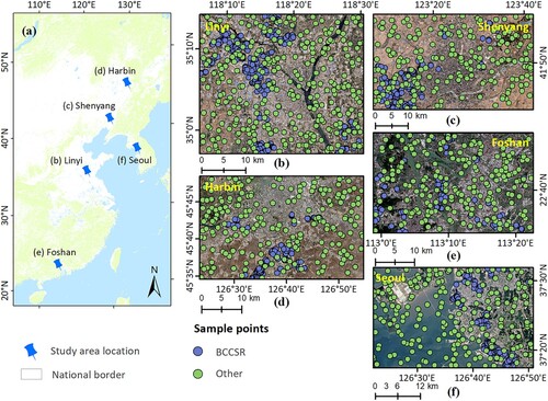
Figure 1. Study area. (a) Location of the study area. (b-f) show the Sentinel-2 images covering the study area and the distribution of sample points.

To address these issues, a new index (BCCSI) was proposed using Sentinel-2 imagery for mapping blue colour-coated steel roofs (BCCSRs) that are widely used in urban areas (Guo et al. 2018). Five typical study areas were selected in China and Southeast Asia. This study aims to: (1) analyse the spectral characteristics of BCCSR and develop a new index (BCCSI) for the unsupervised identification of BCCSR, (2) test the applicability and robustness of BCSSI in different study areas, (3) evaluate the performance of BCCSI by comparison with existing indices and supervised classifiers, and (4) explore the applicability of BCCSI in medium-resolution satellite data, such as Landsat 8 images.

2. Study area and data

2.1. Study area

Five typical study areas, including Linyi (China), Shenyang (China), Harbin (China), Foshan (China), and Seoul (Korea), were selected to develop and evaluate the BCCSI.

Linyi, located in southern Shandong Province, is an important production base of BCCSR in China. It is also known as China’s largest processing and export base for garlic, aluminum, wood, and jade. It has a warm temperate monsoon climate. BCCSRs in this region are mainly used in various industrial and manufacturing plants, which are characterized by large scale and dense distribution (Figure 1b).

Located in the middle of Liaoning Province, Shenyang is an important birthplace of China’s industrialization and is known as the ‘cradle of industry’ in China. It is also known as the transportation and economic center of Northeast China (Sun et al. 2016). It has a rich resource base and industrial base, with major industries including steel, machinery, metallurgy, energy, aviation, and food processing. Like Linyi, BCCSR in Shenyang is characterized by a large scale and dense distribution (Figure 1c).

Located in the middle reaches of the Songhua River, Harbin is an important grain production base in China and is known as the ‘Great Northern Wilderness of China’ (Sun et al. 2020b). It has a cold temperate monsoon climate with long cold winters and short cool summers. BCCSRs in this region appear in small patches (Figure 1d). The wide distribution of cultivated land and buildings poses great challenges to the mapping of BCCSRs in this region.

Foshan is located at the southern end of the Pearl River Delta. It is an important industrial base in South China and is known as the ‘Manufacturing Center of South China’ (Tan et al. 2014). It has a subtropical monsoon climate. BCCSRs in this region occur in small patches (Figure 1e). The dense river network and complex urban background of the region pose a great challenge to BCCSR mapping.

Seoul is the capital of South Korea, located on the southern bank of the Han River, and is known as the ‘urban hub of Northeast Asia’. Its Han River port is one of the largest inland ports in South Korea. It has a temperate humid continental climate (Yoo et al. 2018). Its BCCSR have a scattered distribution and occur in small patches (Figure 1f). The large water bodies and intense human activities increase the complexity of the landscape, making BCCSR mapping difficult.

In general, these five study areas have different BCCSR types and different background conditions. The BCCSRs in Linyi and Shenyang are large and densely distributed. Harbin’s BCCSRs are smaller in size. Moreover, the background conditions of these three regions are relatively simple. In contrast, the BCCSRs in Foshan and Seoul are even smaller and have more complex backgrounds.

2.2. Remote sensing data

In this study, Sentinel-2 multispectral data were used to develop the BCCSI. The Level-1C image was preprocessed to a Level-2A image using the Sen2Cor plugin (version Sen2Cor_v2.11) available from the European Space Agency. We used the nearest neighbor approach to resample the bands with spatial resolutions of 20 and 60 m to 10 m. In addition, to test the cross-sensor applicability of the BCCSI, we downloaded Landsat-8 OLI Level 1 images with a resolution of 30 m. More information about the remote sensing data used is given in Table 1.

Table 1. Remote sensing data used in this study.

Study area	Sentinel 2	Landsat 8
Linyi	S2A, 2022.05.16	2022.05.23
Shenyang	S2B, 2022.02.27	−
Harbin	S2B, 2022.04.28	2022.05.02
Foshan	S2B, 2020.10.11	−
Seoul	S2B, 2021.08.15	2021.10.24

2.3. Reference samples

To provide sufficient data material for the construction and validation of the BCCSI, we selected a total of 4000 samples (including 2000 BCCSR samples and 2000 other samples) from the five study areas. There are 400 BCCSR samples and 400 non-BCCSR samples in each study area. These samples were selected by visually interpreting Google Earth and Esri real-time maps. The samples of each class in Sentinel-2 images were trained (spectral statistical analysis in Sections 3.1 and 3.2) and validated at a 7:3 ratios. The spatial distribution of the sample points is illustrated in Figure 1.

3. Methodology

3.1. Spectral analysis of BCCSRs

We analysed the reflectance of 11 land cover types for each band of Sentinel-2 images. These 11 types include two BCCSR types (dark BCCSR (BCCSRd) and light BCCSR (BCCSRl)), six major land cover types (vegetation, water, bare, high-albedo impervious surface (ISA-ha), medium-albedo impervious surface (ISA-ma), and low-albedo impervious surface (ISA-la)), and three special types (red-roof building (RRB), urban green plastic cover (UGPC), and building shadow (BS)).

ISA-ha is commonly used in high-speed railway stations and airport buildings (Figure 2c), while ISA-la is often used in urban asphalt roads (Figure 2e). RRBs are mainly used in factory buildings and tiled residential buildings (Figure 2f), including red tile roof and red colour-coated steel roof. UGPC is used to prevent dust from urban development and is a common material in urban construction (Cao and Huang 2022) (Figure 2g). In addition to ISA, RRBs and water bodies are widely distributed in Foshan and Seoul, while BS and bare land are widely distributed in Harbin, Shenyang, and Linyi. Moreover, UGPC is common in Linyi and Shenyang, which may lead to confusion with BCCSR. Hence, we specifically listed them for further study. We plotted the spectral profiles for 11 land cover types utilizing sample point data from five study areas (Figure 3).

Figure 2. Examples of (a) BCCSRd, (b) BCCSRl, (c) ISA-ha, (d) ISA-ma, (e) ISA-la; (f) RRB, (g) UGPC, and (h) BS.

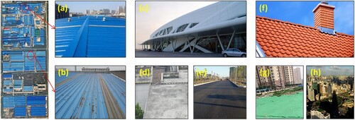
Figure 3. Spectral profiles based on Sentinel-2 images. (a) Average spectral profiles of six common land cover types (i.e. vegetation, water, bare, ISA-ha, ISA-ma, ISA-la); (b) Average spectral profiles of three special land cover types (i.e. RRB, UGPC, BS). Note that BCCSRl and BCCSRd are marked with orange–red lines.

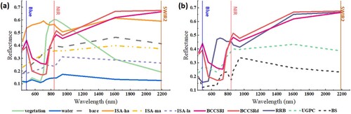
The spectral profiles of BCCSRs (BCCSRl and BCCSRd) have obvious characteristics, which are different from typical land cover types such as vegetation, water and bare soil. The BCCSR drops from the blue band (490 nm) to the red band (665 nm), then rises again to the near-infrared (NIR) band (842 nm) and reaches its highest reflectance at the short-wave infrared (SWIR) band (2190 nm). The reflectance peak of the BCCSR appeared in the blue and NIR bands, and the absorption peak appeared in the red band. Therefore, the BCCSR presents an obvious ‘U-shaped valley’ between the blue and NIR bands (Guo et al. 2018). The BCCSR and ISA-ha have high reflectivity in blue, NIR and SWIR bands. The BCCSR has strong absorption of vegetation, water bodies, ISA-ma and ISA-la in the green and red bands, and strongly reflects of vegetation in the NIR band. In addition, the reverse-colour peak of RRB occurs near the NIR band, but its absorption peak occurs near the blue band. BS is similar in shape and size to the reflected spectrum of water, and has low reflectance at blue, green and red bands. In addition, the UGPC and BCCSR reflectance spectra are very similar in shape and size. As a result, BCCSR seems to be difficult to distinguish from UGPC, especially BCCSRl.

3.2. Separation analysis of BCCSRs

Figure 4 shows the spectral reflectance for each land cover type. The M-index (Xun et al. 2021; Zhang et al. 2022) was chosen to measure the separability of BCCSRs and other land covers. It was calculated as follows. (1) $M={\displaystyle \frac{|{\mu }_1-{\mu }_2|}{{\sigma }_1+{\sigma }_2}}$(1) where ${\mu }_1$ and ${\mu }_2$ denote the mean of Class 1 and Class 2, respectively. ${\sigma }_1$ and ${\sigma }_2$ denote the standard deviation of Class 1 and Class 2, respectively. When the M value is greater than 1, it indicates good separability; otherwise, it indicates poor separability.

Figure 4. Reflectance of 11 land cover types in Sentinel-2 bands.

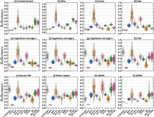
As seen in Figures 3 and 4, the BCCSR drops from the blue band to the green band and reaches maximum absorption at the red band. These features can be used to separate the BCCSR from the ISA and bare soil. It is not difficult to see from Figure 4 (b) that the blue band is a good indicator, which can highlight the BCCSR while suppressing the ISA (ISA-ma and ISA-la) and bare soil. As can be seen in Figure 4 (c) and (d), the green and red bands are very useful for distinguishing BCCSR from ISA-ha. Therefore, the difference of blue and green bands (blue–green) and the difference of blue and red bands (blue-red) can effectively distinguish BCCSRs from ISA and bare land. Figure 3 (b) shows that the above two differences can also highlight the BCCSR and suppress the RRB and BS. Thus, to separate the above land cover types, we designed a Blue normalized index (BNI), which is calculated as follows: (2) $BNI={\displaystyle \frac{2{\rho }_{Blue}-{\rho }_{Green}-{\rho }_{Red}}{2{\rho }_{Blue}+{\rho }_{Green}+{\rho }_{Red}}}$(2) The index ensures that the value of BCCSR is greater than 0, while the values of ISA, bare soil, RRB and BS are less than 0. Therefore, BNI can be used to separate BCCSR from ISA, bare soil, RRB and BS. Furthermore, it can make the values of vegetation and water near zero.

The above analysis suggests that blue–green and blue-red are available to distinguish BCCSR from ISA, bare soil, RRB, and BS. However, they are not sufficient to suppress water, vegetation and UGPC. As shown in Figure 4, water and vegetation have similar reflectance in the blue, green and red bands. The reflectance spectra of UGPC and BCCSR are very similar in shape and size. Therefore, it is hard to inhibit them with blue–green and blue-red. In addition, the SWIR band is very sensitive to water (Zhang et al. 2022); vegetation and water had stronger absorption in the SWIR2 band, while BCCSR had stronger reflectance in the SWIR2 band. Figure 2 (l) shows that the SWIR2 band is very useful for distinguishing BCCSR from some natural surfaces (such as vegetation and water). The SWIR2 band can separate BCCSRl from vegetation and water, with M-indices of 3.23 and 3.66, respectively (Table 2). It is not difficult to see from Figure 4 (b) and (l) that the blue band and SWIR2 could highlight BCCSR and suppress UGPC. The blue band is the optimal indicator to distinguish BCCSRl from UGPC with an M-index of 2.74, and the SWIR2 band is the optimal indicator to distinguish BCCSRd from UGPC with an M-index of 2.45 (Table 2).

Table 2. Separability between BCCSR and other land covers.

	B1	B2	B3	B4	B5	B6	B7	B8	B8A	B9	B11	B12
BCCSRl and vegetation	4.37	6.78	3.65	3.34	1.26	2.28	1.73	1.24	1.07	1.17	2.61	3.23
BCCSRl and water	3.70	5.12	3.13	3.53	2.87	0.95	1.44	1.76	1.87	1.65	3.75	3.66
BCCSRl and bare	2.67	3.20	0.63	0.55	0.86	1.00	0.12	0.54	0.69	0.58	1.03	1.29
BCCSRl and ISA-ha	0.38	0.56	1.61	1.97	2.12	2.12	1.05	0.58	0.39	0.38	0.02	0.23
BCCSRl and ISA-ma	2.29	2.85	0.29	0.83	1.37	1.53	0.58	1.28	1.67	1.44	2.02	1.91
BCCSRl and ISA-la	2.81	4.46	1.97	0.82	0.45	0.16	1.60	2.60	2.47	1.55	2.66	2.49
BCCSRl and RRB	2.65	4.85	2.83	2.85	2.54	2.47	0.62	0.11	0.62	0.49	0.18	0.01
BCCSRl and UGPC	2.27	2.74	0.93	0.61	0.09	0.65	0.60	1.02	1.09	0.83	1.63	1.75
BCCSRl and BS	2.48	5.10	3.23	1.98	0.73	0.37	1.58	2.79	2.37	1.44	2.67	2.51
BCCSRd and vegetation	4.34	6.39	1.70	2.05	0.52	3.63	1.61	0.98	0.77	0.94	3.31	4.63
BCCSRd and water	3.65	4.70	1.56	2.37	1.59	0.41	1.26	1.78	2.01	1.76	4.54	5.22
BCCSRd and bare	2.59	2.71	0.85	1.79	1.99	2.00	0.03	0.65	0.91	0.76	1.47	1.72
BCCSRd and ISA-ha	0.46	0.86	2.43	2.81	2.93	2.92	1.02	0.44	0.19	0.21	0.22	0.31
BCCSRd and ISA-ma	2.18	2.28	1.77	2.91	3.77	3.86	0.36	1.37	2.00	1.74	2.76	2.73
BCCSRd and ISA-la	2.72	3.94	0.03	1.04	1.29	1.22	1.27	2.56	2.72	1.77	3.37	3.44
BCCSRd and RRB	2.57	4.36	0.91	5.29	4.22	4.02	0.65	0.30	0.93	0.73	0.10	0.04
BCCSRd and UGPC	2.16	2.11	1.80	1.74	2.58	2.68	0.39	1.14	1.42	1.13	2.30	2.45
BCCSRd and BS	2.39	4.67	1.65	0.77	0.48	0.72	1.28	2.74	2.60	1.68	3.33	3.39

3.3. Development of BCCSI

After the analysis of separability, the blue colour-coated steel roof index (BCCSI) was constructed according to three aspects: (1) As a combination of blue–green and blue-red, the BNI index can be used to separate BCCSR from ISA, bare, RRB and BS. (2) The SWIR band is very sensitive to water (Zhang et al. 2022) and is very useful for distinguishing BCCSR from some natural surfaces (such as vegetation and water). The SWIR2 band is a good indicator that can separate BCCSRl from vegetation and water. (3) The blue band and SWIR2 band can highlight the BCCSR and suppress the UGPC. The blue and SWIR2 bands are the best indicators that can separate BCCSRd and BCCSRl from UGPC, respectively. Based on this principle, the BCCSI was developed to highlight the BCCSR and suppress the environmental background. The formula for the BCCSI is: (3) $BCCSI=100\times {\rho }_{Blue}\times {\rho }_{SWIR2}\times {\displaystyle \frac{2{\rho }_{Blue}-{\rho }_{Green}-{\rho }_{Red}}{2{\rho }_{Blue}+{\rho }_{Green}+{\rho }_{Red}}}$(3) In this formula, ${\rho }_{Blue}$, ${\rho }_{Green}$, ${\rho }_{Red}$, and ${\rho }_{SWIR2}$ represent the reflectance of the blue, green, red, and SWIR2 bands, respectively, ranging from 0 to 1. The SWIR2 band and blue band were used to further suppress vegetation and water information and make the UGPC value even lower. The multiplier of 100 is used to stretch the BCCSI to a larger range. Thus, the BCCSI may be an efficient indicator to both highlight BCCSR and suppress the complex urban background condition.

3.4. Validation

3.4.1. Comparison with existing VIs

Six VIs, including normalized built-up area index (NDBI) (Zha, Gao, and NI 2003), blueness index (BI) (Viscarra Rossel et al. 2006; Escadafal 1993), normalized difference blue building index (NDBBI), logical blue building index (LBBI), enhanced blue building index (EBBI) (Samat et al. 2022), and ‘blue steel tile’ – roofed building index (BSTBI) (Guo et al. 2018) were selected to compare with the BCCSI. Their calculation equations are: (4) $NDBI={\displaystyle \frac{{\rho }_{SWIR1}-{\rho }_{NIR}}{{\rho }_{SWIR1}+{\rho }_{NIR}}}$(4) (5) $BI={\displaystyle \frac{{\rho }_{Blue}}{{\rho }_{Blue}+{\rho }_{Green}+{\rho }_{Red}}}$(5) (6) $NDBBI={\displaystyle \frac{{\rho }_{Blue}-{\rho }_{Green}}{{\rho }_{Blue}+{\rho }_{Green}}}$(6) (7) $LBBI=\{\begin{array}{cc}1& {\rho }_{Blue}>{\rho }_{Green}\mathrm{\&}{\rho }_{Blue}>{\rho }_{Red}\mathrm{\&}{\rho }_{NIR}>{\rho }_{Green}\mathrm{\&}{\rho }_{NIR}>{\rho }_{Red}\\ 0& other\end{array}$(7) (8) $EBBI={\displaystyle \frac{2{\rho }_{Blue}-({\rho }_{Green}+{\rho }_{Red})}{2{\rho }_{Blue}+({\rho }_{Green}+{\rho }_{Red})}}$(8) (9) $BSTBI=\left({\displaystyle \frac{{\lambda }_{Green}-{\lambda }_{Blue}}{{\lambda }_{NIR}-{\lambda }_{Blue}}\times {\rho }_{Blue}+{\displaystyle \frac{{\lambda }_{NIR}-{\lambda }_{Green}}{{\lambda }_{NIR}-{\lambda }_{Blue}}\times {\rho }_{NIR}-{\rho }_{Green}}}\right)\times {\rho }_{SWIR2}$(9) where ${\rho }_{Blue}$, ${\rho }_{Green}$, ${\rho }_{Red}$, ${\rho }_{NIR}$, ${\rho }_{SWIR1}$, and ${\rho }_{SWIR2}$ represent the reflectance of the blue, green, NIR, SWIR1, and SWIR2 bands. ${\lambda }_{Blue}$, ${\lambda }_{Green}$, and ${\lambda }_{NIR}$ represent the wavelengths of the blue, green, and NIR bands, which are 492.4 (492.1) nm, 559.8 (559) nm, and 832.8 (832.9) nm in the Sentinel-2A(B) images, respectively.

3.4.2. Visual evaluation

Visual evaluation enables intuitively analysis the ability of different indices to highlight target and suppress background (Zhang et al. 2022). To obtain an objective result, we set up two rules. First, all index images should be visualized in the same stretching method. Considering the effect of noise on visual evaluation, we used a percentage truncated stretching method to display the indexed images. Second, the five study areas, including Linyi, Shenyang, Harbin, Foshan, and Seoul, were visually compared in both large and small area.

3.4.3. Comparison with ML methods

Two commonly used supervised classifiers (Maurya, Mahajan, and Chaube 2021), including neural network (NN) and support vector machine (SVM), were chosen for comparison with our proposed BCCSI. The NN model requires setting the hidden layer number and the training iteration number. In this study, they were set to 1 and 1000, respectively. The radial basis function was chosen as the kernel function for the SVM model. To train the SVM classifier, it is required to set kernel function gamma, penalty parameter and pyramid levels. In this study, they were set to 0.5, 100 and 0, respectively.

3.4.4. Accuracy validation

Overall accuracy (OA), producer’s accuracy (PA), user’s accuracy (UA), and F1 score (F1) were chosen to evaluate the precision (Hou et al. 2022; Zhang et al. 2022). They are calculated as follows: (10) $OA={\displaystyle \frac{TP+TN}{TP+FN+FP+TN}}$(10) (11) $UA={\displaystyle \frac{TP}{TP+FP}}$(11) (12) $PA={\displaystyle \frac{TP}{TP+FN}}$(12) (13) $F1=2\times {\displaystyle \frac{UA\times PA}{UA+PA}}$(13) where TP, TN, FP, and FN denote the number of true-positive, true-negative, false-positive, and false-negative samples, respectively.

4. Results

4.1. Comparison with existing VIs

This section mainly explores the BCCSR identification performance of the seven indices in the five study areas. In the visual evaluation results, brown correlated with BCCSRs, while dark green correlated with background. Additionally, visual comparison analysis was performed at two spatial scales to clearly compare the overall and detailed performance of each index. In addition, using 4000 sample points selected by visual interpretation (see Section 2.3), we analysed the separability of BCCSRs from other land covers for each index.

4.1.1. Visibility comparison

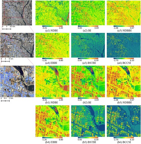
Figure 5 shows the visualization results for the six indices in Linyi. The NDBI had the worst ability to highlight BCCSRs, and the ISA and water bodies were confused with BCCSRs (Figure 5 (a1) and (b1)). In the BI, NDBBI and EBBI images, many background conditions were incorrectly highlighted, especially ISA (Figure 5 (a2–a4) and (b2–b4)). BSTBI effectively highlighted the BCCSR (Figure 5 (a5) and (b5)), however, BCCSI showed more obvious advantages in suppressing the background (Figure 5 (a6) and (b6)).

Figure 5. Visualization results for the six indices in Linyi.

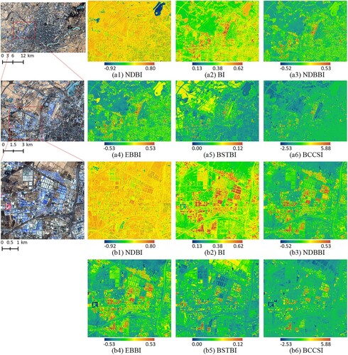
Figure 6 shows the visualization results for the six indices in Shenyang. The NDBI incorrectly highlighted a large amount of the background conditions (Figure 6 (a1) and (b1)). In the BI, NDBBI and EBBI images, the complex urban background was confused with the BCCSRs, especially ISA and BS (Figure 6 (a2–a4) and (b2–b4)). In the BI, NDBBI and EBBI images, the complex urban background was confused with the BCCSRs, especially ISA and BS (Figure 6 (a2–a4) and (b2–b4)). Furthermore, both BI and EBBI mistakenly identified water bodies as BCCSRs. In the BSTBI image, many bare land pixels were incorrectly highlighted, and RRB information could not be effectively suppressed. The BCCSI performed better in highlighting BCCSR information and suppressing complex urban backgrounds (Figure 6 (a6) and (b6)).

Figure 6. Visualization results for the six indices in Shenyang.

Figure 7 illustrates the visualization results for the six indices in Harbin. It is evident that NDBI was ineffective in highlighting the BCCSR (Figure 7 (a1) and (b1)). BI, NDBBI, EBBI, and BSTBI were effective in highlighting BCCSRs; however, some background environmental pixels were also incorrectly highlighted, including ISA-ha, bare land, and BS (Figure 7 (a2–a5) and (b2–b5)). As demonstrated in Figure 7 (a6) and (b6), the BCCSI highlighted the BCCSRs from the background accurately and was more effective in suppressing background conditions.

Figure 7. Visualization results for the six indices in Harbin.

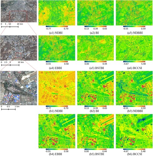
Figure 8 displays the visualization results for the six indices in Foshan. Unlike the above three study areas, Foshan has a smaller BCCSR and more complex background conditions. The complex and scattered pattern poses challenges to most indices. At a large scale, BCCSI, BI, and EBBI performed better in highlighting the BCCSR area and suppressing the background compared to other indices (Figure 8 (a2–a6)). NDBBI and BSTBI also highlighted BCCSRs, but they erroneously highlighted some land covers, such as ISA and RRB. As shown in Figure 8 (b2–b4), ISA and BS were confused with BCCSRs in BI, NDBBI, and EBBI. As shown in Figure 8 (b5), RRB and bare land were confused with BCCSRs in the BSTBI. As seen in Figure 8 (b6), the BCCSI effectively suppressed ISA, BS, RRB, and bare soil information.

Figure 8. Visualization results for the six indices in Foshan.

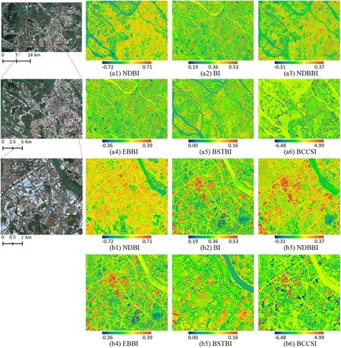
Figure 9 shows the visualization results of the six indices in Seoul. The background condition of Foshan is similar to that of Seoul, but the size of BCCSRs in Seoul is smaller. At a large scale, although BI, NDBBI, and EBBI highlighted the BCCSRs, many water pixels were incorrectly highlighted (Figure 9 (a1–a6)). BCCSI, BSTBI, and NDBI suppressed water bodies effectively, but NDBI failed to highlight BCCSRs from urban backgrounds (such as ISA), and BSTBI mistakenly highlighted some land cover information, such as RRB, bare land, and vegetation. As shown in Figure 9 (b2–b4), ISA-ha and water bodies were confused with BCCSRs in BI, NDBBI, and EBBI. As shown in Figure 9 b(5), RRB and vegetation were confused with BCCSRs in the BSTBI. Overall, BCCSI proved to be more effective in highlighting BCCSRs and suppressing background conditions.

Figure 9. Visualization results for the six indices in Seoul.

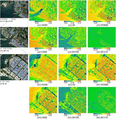
The BCCSI showed superior and robust performance in the five typical study areas. First, the other indices only excelled in highlighting BCCSRs in some study areas but not for all study areas. For example, the BSTBI performed well in Linyi but had poor identification results in the other four study areas. Second, BCCSI effectively suppressed various types of background conditions, while other indices were easily influenced by complex urban backgrounds. For example, water is confused with BCCSRs in BI and EBBI.

4.1.2. Comparison of the separability of the indices

Figure 10 shows the statistical distribution of various land covers for the six indices, and Table 3 lists the M-indices of BCCSRd and BCCSRl with other land covers. It is easy to see that BCCSI was the best index to distinguish BCCSRd and BCCSRl from other land covers. The BI and EBBI were effective in highlighting the BCCSR but could not distinguish water bodies, BS and BCCSR. For the BI and EBBI indices, the M-index of BCCSR and water bodies was less than 0.1, and the M-index of BCCSR and BS was less than 1. The BSTBI suppressed water information, but RRB, vegetation and bare land were confused with BCCSRs, especially RRB. The M-indices of BCCSRl and BCCSRd with RRB were 0.50 and 0.29, respectively. The NDBBI failed to effectively separate BS and BCCSR (M-index less than 1), which limits its ability to identify BCCSRs in urban areas. However, using BCCSI, BCCSRs (including BCCSRl and BCCSRd) was well distinguished from all other land covers, with separation indices greater than 1.

Figure 10. Statistical distribution of each land cover type for the six indices.

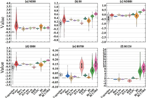
Table 3. Separability of BCCSR and other land covers on the six indices.

	NDBI	BI	NDBBI	EBBI	BSTBI	BCCSI
BCCSRl and vegetation	5.22	2.32	1.37	1.32	1.05	1.98
BCCSRl and water	0.13	0.05	0.93	0.07	1.69	1.63
BCCSRl and bare	0.37	4.40	4.17	4.67	0.99	2.02
BCCSRl and ISA-ha	0.76	2.67	2.61	2.74	1.45	1.76
BCCSRl and ISA-ma	0.87	3.78	3.58	4.01	1.55	2.13
BCCSRl and ISA-la	0.09	3.18	2.96	3.26	1.77	2.02
BCCSRl and RRB	0.34	5.02	1.95	5.10	0.50	2.21
BCCSRl and UGPC	0.76	0.03	0.09	1.61	0.80	1.68
BCCSRl and BS	0.86	0.01	0.33	0.54	1.65	1.97
BCCSRd and vegetation	4.62	3.29	2.03	1.68	2.40	3.84
BCCSRd and water	0.13	0.05	1.48	0.09	3.14	3.02
BCCSRd and bare	0.46	7.46	7.13	7.99	1.12	3.62
BCCSRd and ISA-ha	0.79	5.41	5.39	5.64	2.60	3.12
BCCSRd and ISA-ma	0.90	6.98	6.69	7.59	3.09	3.97
BCCSRd and ISA-la	0.21	5.87	5.47	6.02	3.36	3.88
BCCSRd and RRB	0.15	7.53	4.42	7.40	0.29	3.78
BCCSRd and UGPC	0.80	1.89	0.04	3.93	1.61	3.26
BCCSRd and BS	0.73	0.05	0.56	0.76	3.12	3.80

4.2. BCCSR mapping

Figure 11 shows the mapping accuracy of the six indices at different thresholds. It is not difficult to see that the BCCSI achieved the highest mapping accuracy in all study areas. The NDBI showed the lowest mapping accuracy in all five study areas. The BI and EBBI performed well in Linyi, Shenyang, and Harbin, but poorly in Foshan and Seoul. The NDBB and BSTBI performed better in Linyi, Harbin, and Seoul but worse in Shenyang and Foshan. The BCCSI was effective in identifying BCCSRs in all five typical study areas. The accuracy of BCCSI was higher in Linyi, Shenyang, and Harbin than in Foshan and Seoul. This may be because Foshan and Seoul have smaller BCCSRs, dense river networks (large areas of water) and complex urban backgrounds. Table 4 shows the quantitative mapping accuracy of the six indices at the optimal threshold. The BCCSI achieved the best accuracy in all five study areas, with an OA of 93.88%−98.82% and an F1 of 93.18%−98.58%.

Figure 11. The BCCSR mapping accuracy curves of the six indices in (a) Linyi, (b) Shenyang, (c) Harbin, (d) Foshan, and (e) Seoul.

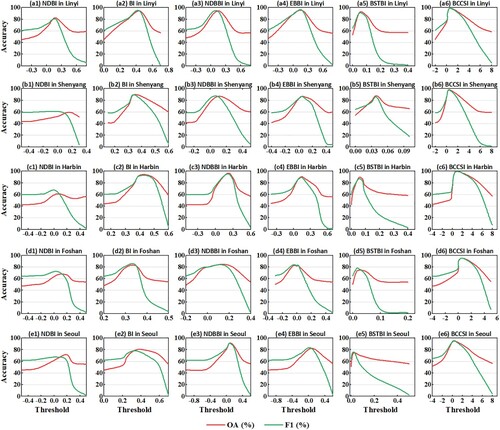
Table 4. Accuracy of the six indices at the optimal threshold.

Study area	Indices	Thresholds	UA (%)	PA (%)	OA (%)	F1 (%)
Linyi	NDBI	0.10	66.43	94.68	77.24	78.08
	BI	0.45	92.41	93.02	93.75	92.72
	NDBBI	0.15	91.19	95.24	94.05	93.17
	LBBI	−	98.69	97.41	98.31	98.05
	EBBI	0.20	91.69	95.82	94.42	93.71
	BSTBI	0.05	86.25	96.17	91.62	90.94
	BCCSI	0.53	97.41	99.34	98.58	98.37
Shenyang	NDBI	0.12	49.72	63.57	58.53	55.80
	BI	0.35	80.92	98.59	89.77	88.89
	NDBBI	0.05	77.78	96.55	86.57	86.15
	LBBI	−	98.58	97.20	98.25	97.89
	EBBI	0.05	79.55	94.59	86.50	86.42
	BSTBI	0.04	88.81	80.95	87.64	84.70
	BCCSI	0.50	97.89	99.29	98.82	98.58
Harbin	NDBI	0.05	52.65	84.40	64.03	64.85
	BI	0.40	89.54	94.48	93.04	91.95
	NDBBI	0.20	96.35	93.62	95.83	94.96
	LBBI	−	96.55	92.11	95.10	94.28
	EBBI	0.15	85.53	92.52	90.48	88.89
	BSTBI	0.05	79.65	94.48	87.92	86.44
	BCCSI	0.55	97.90	96.55	97.63	97.22
Foshan	NDBI	0.18	70.93	46.92	66.43	56.48
	BI	0.35	74.29	91.55	81.96	82.02
	NDBBI	0.00	69.15	94.20	79.69	79.75
	LBBI	−	95.56	87.76	92.05	91.49
	EBBI	0.02	77.38	89.66	82.45	83.07
	BSTBI	0.02	66.67	92.86	74.14	77.61
	BCCSI	0.75	97.73	91.49	94.88	94.51
Seoul	NDBI	0.20	78.43	49.38	71.27	60.61
	BI	0.35	70.59	86.67	79.77	77.81
	NDBBI	0.08	93.06	88.95	91.23	90.96
	LBBI	−	94.58	87.22	91.69	90.75
	EBBI	0.08	75.23	89.94	82.03	81.93
	BSTBI	0.03	67.77	83.63	74.67	74.87
	BCCSI	0.80	96.91	89.71	93.88	93.18

BCCSR mapping was performed using the optimal thresholds of each index. The NDBI index was not effective in identifying BCCSRs, so its results are not presented. As shown in Figure S1–S5, the BCCSI was able to accurately identify BCCSRs in the five study areas. The other five indices only valid for BCCSR identification in some study areas, but they cannot achieve robust BCCSR identification results in all study areas. For example, the NDBBI can effectively identify BCCSRs in Seoul but not in Shenyang and Foshan. In addition, BCCSI has a clear advantage in suppressing complex background conditions, while other indices misidentify other land covers. For example, as shown in Figure S1 (a1–a3) and (b1–b3), BI, NDBBI and EBBI misidentified water bodies as BCCSRs, and some BCCSRs were not effectively identified. As shown in Figures S2 (b4) and S3 (b4), the BSTBI incorrectly identified the RRB as the BCCSR. As shown in Figures S3 and S4 (a1–a4) and (b1–b4), the BI, NDBBI, LBBI, and EBBI incorrectly identified the BS as BCCSRs. As shown in Figures S4 and S5, the BI, LBBI and EBBI incorrectly identified water bodies and BS, and the BSTBI labelled some vegetation and bare soil as BCCSRs. In general, BCCSI was able to accurately identify BCCSRs from various complex backgrounds. Shenyang, Foshan, and Seoul are the regions with the most obvious gap between the BCCSI and other indices. This is primarily due to the complex and scattered BCCSRs in these regions, with large water bodies and complex urban backgrounds.

4.3. Comparison with ML methods

Figure 12 shows the BCCSR identification results of the ML algorithm in the five study areas. In general, the ML algorithm performed well in BCCSR identification, and achieved higher accuracy than the BCCSI in some study areas. As shown in Table 5, the BCCSR mapping accuracy of the ML algorithms in Linyi, Harbin, and Foshan was higher than that of the BCCSI, especially the SVM algorithm. The accuracies of the ML algorithms and the BCCSI were similar in Shenyang and Seoul. However, the accuracy of the ML algorithm depends heavily on the quantity and quality of sample, and the collection of training samples is time-consuming and labour intensive, especially for large-scale mapping (Zhang et al. 2022; Xun et al. 2021). The BCCSI achieved a similar BCCSR mapping accuracy as the ML algorithm without the need for sample points. Overall, the BCCSI has more efficiency and potential for large-scale BCCSR mapping.

Figure 12. BCCSR mapping results using ML algorithms and the BCCSI in the five study areas.

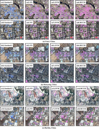
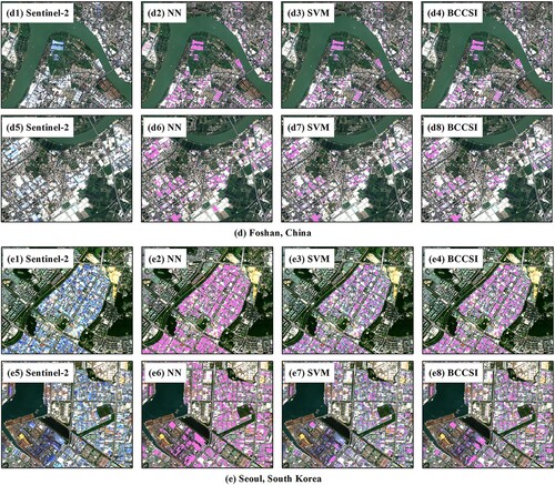
Table 5. Quantitative accuracy of the ML algorithms in the five study areas.

Study area	Indices	UA (%)	PA (%)	OA (%)	F1 (%)	Thresholds
Linyi	NN	98.99	98.01	98.72	98.50	−
	SVM	98.35	99.00	98.86	98.68	−
	BCCSI	97.41	99.34	98.58	98.37	0.53
Shenyang	NN	97.20	98.58	98.24	97.89	−
	SVM	97.87	98.57	98.53	98.22	−
	BCCSI	97.89	99.29	98.82	98.58	0.50
Harbin	NN	97.89	97.20	97.91	97.54	−
	SVM	99.29	98.58	99.10	98.93	−
	BCCSI	97.90	96.55	97.63	97.22	0.55
Foshan	NN	98.48	96.30	97.54	97.38	−
	SVM	99.24	94.20	96.88	96.65	−
	BCCSI	97.73	91.49	94.88	94.51	0.75
Seoul	NN	89.44	96.99	93.55	93.06	−
	SVM	97.52	94.01	96.19	95.73	−
	BCCSI	96.91	89.71	93.88	93.18	0.80

5. Discussion

5.1. Robustness of the threshold

As shown in Table 5, the optimal threshold of BCCSI in the five study areas ranges from 0.50 to 0.80. The BCCSI thresholds in Seoul and Foshan were higher than those in Linyi, Shenyang, and Harbin. This is mainly because Seoul and Foshan have a large amount of vegetation and water bodies, which tends to cause confusion with BCCSRs. A larger BCCSI threshold can avoid interference of these information. Table 6 shows the mapping accuracy of BCCSI under different thresholds. The BCCSI showed strong robustness in the five typical study areas. Even if the threshold of BCCSI was 0.1, the OA (F1) was greater than 91.08% (89.96%). In addition, within the optimal threshold of ±0.2, the OA (F1) of Linyi, Shenyang, and Harbin BCCSIs was greater than 94.57% (95.05%), and the OA (F1) of Foshan and Seoul BCCSIs was greater than 92.49% (91.38%). Overall, the BCCSI achieved robust results even when the thresholds differed significantly from the optimal thresholds.

Table 6. The accuracy of BCCSR mapping at different BCCSI thresholds.

Study area	Accuracy	BCCSI=										Best threshold
		0.1	0.2	0.3	0.4	0.5	0.6	0.7	0.8	0.9	1.0
Linyi	OA (%)	90.68	93.59	95.75	97.24	98.18	98.04	97.29	96.78	96.26	95.65	98.58
	F1 (%)	90.17	93.07	95.47	97.10	98.09	97.62	96.69	96.17	95.61	94.94	98.37
Shenyang	OA (%)	90.84	95.09	97.51	98.40	98.82	98.00	97.73	97.26	96.85	96.28	98.82
	F1 (%)	91.13	94.85	97.13	98.10	98.58	97.51	97.13	96.44	95.78	95.04	98.58
Harbin	OA (%)	90.84	92.54	94.57	96.20	97.35	97.48	95.98	95.11	94.12	92.76	97.63
	F1 (%)	91.71	93.42	95.05	96.09	96.97	96.98	95.38	94.51	93.34	92.10	97.22
Foshan	OA (%)	90.88	92.59	93.61	93.92	93.99	94.46	94.88	93.84	93.46	92.59	94.88
	F1 (%)	91.11	92.66	93.53	93.74	93.84	94.30	94.51	93.44	92.66	91.34	94.51
Seoul	OA (%)	91.08	91.55	91.87	92.30	92.86	93.38	93.84	93.88	93.43	92.49	93.88
	F1 (%)	89.96	90.61	91.22	91.78	92.35	92.77	93.10	93.18	92.49	91.83	93.18

Based on these results, we suggest the use of thresholds within the optimal threshold ±0.2 (0.3–1.0) for accurate BCCSR mapping. However, for large-scale BCCSR mapping, we suggest that researchers adjust the threshold of the BCCSI according to the study area characteristics and BCCSR types.

5.2. Applicability of BCCSI in Landsat-8 images

We discussed the applicability of BCCSI to Landsat images (Figure S6). Figure S7 shows the accuracy curve of the BCCSR mapping results of Landsat-8 images under different BCCSI thresholds. Overall, the BCCSI results of Landsat-8 were satisfactory. The optimal thresholds of the BCCSI in Linyi, Harbin and Seoul were 0.51, 0.47 and 0.74, respectively. In addition, the identification accuracy of BCCSRs in Linyi and Harbin was higher than that in Seoul. Under the optimal threshold, the OAs (F1) of the three study areas were 98.32% (97.98%), 96.16% (95.78%) and 86.67% (86.01%), respectively. In Linyi and Harbin, the BCCSI of Landsat-8 showed similar performance to that of Sentinel-2 (Figure 11 (a6) and (c6)), with the highest overall accuracy exceeding 98% and 95%, respectively. In Seoul, the BCCSI results in Landsat-8 images exceeded 85%, approximately 7% lower than in Sentinel-2 images (Figure 11 (e6)). Overall, BCCSI was applicable to Landsat-8 data. The BCCSI has the potential to be applied to other satellite images as long as the blue, green, red and SWIR2 bands are available.

5.3. Advantages and limitations of the BCCSI

5.3.1. Advantages of the BCCSI

Timely and accurately obtaining the spatial distribution information of BCCSRs is important for understanding the potential effects of coated steel on human health and the environment. At present, machine learning algorithms have proven to be an effective method for identifying BCCSRs (Sun et al. 2020). However, the above methods are supervised classifiers, whose accuracy depends mainly on the quantity and quality of the samples (Hou et al. 2022; Xun et al. 2021). Collecting samples is time-consuming and labour intensive, especially for large-scale mapping (Zhang et al. 2022). In addition, the existing indices are not always effective in highlighting BCCSR and suppressing the background conditions. Therefore, we developed the BCCSI using Sentinel 2 data. The index was able to map BCCSRs in five typical study areas selected from China and Korea, and compared with existing methods, BCCSI has several advantages.

First, we fully considered the spectral reflectance and absorption of BCCSRs, and the constructed BCCSI better highlighted the BCCSR pixels and suppressed the background environment pixels. According to spectral analysis (Figure 3), BCCSRs present an obvious ‘U-shaped valley’ between the blue and NIR bands, which is consistent with previous findings (Guo et al. 2018). Therefore, we constructed an important index BNI to exclude land covers with increasing spectral reflectance from blue to red bands, such as bare soil and RRB. In existing studies, the BI, NDBBI and EBBI indices only consider this characteristic. Moreover, to further exclude interference from ISA, water bodies, vegetation and UGPC, we considered the blue band and SWIR2 band in the BCCSI, where the BCCSR reaches its reflectance peak in blue band and its highest reflectance in SWIR2 band. In contrast, existing indices either fail to highlight BCCSRs (such as NDBI) or fail to suppress background conditions (such as BI, NDBBI, LBBI, and BSTBI). This advantage of the BCCSI is demonstrated by the separation between the BCCSR (BCCSRl and BCCSRd) and other land covers in Figure 10.

Second, compared with the ML algorithms, the proposed BCCSI performed high-precision BCCSR mapping without human participation. Figure 12 and Table 5 show that the BCCSI achieved the comparable accuracy to the ML algorithms, while avoiding time-consuming and laborious sample selection. In addition, Table 8 shows that the BCCSI showed strong robustness in the five typical study areas. Even if the threshold differs greatly from the optimal threshold (e.g. BCCSI = 0.1), OA (F1) can be greater than 91.08% (89.96%). Therefore, the BCCSI is more efficient and has the potential to be used for BCCSR identification and dynamic monitoring in the absence or lack of training samples.

Third, the proposed BCCSI can be applied to medium-resolution images with four major bands (blue, green, red and SWIR2), such as Landsat-8 images. We found some common spectral characteristics of BCCSRs in Landsat-8 images and Sentinel-2 images (Figure S6). Our results showed that the two data sources had comparable accuracy in Linyi and Harbin, although the accuracy in Seoul using Landsat-8 images was slightly lower than that of Sentinel-2 images (Table 2). This is mainly because the spatial resolution limits the performance of Landsat-8 images. In addition, we found that the optimal BCCSI thresholds of Landsat-8 and Sentinel-2 images were basically the same in the three study areas, which further indicated the strong robustness of the BCCSI index in different study areas.

5.3.2. Limitations of the BCCSI

Despite the above advantages of the proposed method, there are still some limitations and uncertainties in the mapping of BCCSRs. First, this study fully explored the potential of BCCSI to identify BCCSRs in urban areas; however, the size of BCCSRs is smaller in rural‒urban or rural areas. It has been reported that the BCCSR is a popular material in poor or rural areas (Lamnatou et al. 2018; Kültür and Türkeri 2012). Obtaining BCCSR information in these areas is important for understanding the potential environmental impacts of colour-coated steel materials. Therefore, it is necessary to explore the applicability of BCCSI to higher resolution images (such as WordView-3) in the future. Second, some organic surfaces with colors similar to BCCSR may be incorrectly identified as BCCSRs, and some BCCSRs covered with dust or oil will be missed. For example, runways and courts coated with blue organic paint may be confused with BCCSRs because the organic paint has similar absorption characteristics to BCCSR (Guo and Li 2020). In addition, the BCCSR of ports are covered with dust or oil and cannot be effectively identified (Guo et al. 2018), such as Incheon Port in Seoul (Figure S5 (b5)). Future research will aim to explore more features to highlight the BCCSRs to increase the separability from other surfaces. These limitations need to be addressed in future work.

6. Conclusions

BCCSRs are rapidly expanding worldwide because of their low cost and easy maintenance, but they also have a series of negative impacts on local ecology. Therefore, timely and accurate acquisition of BCCSR spatial distribution information is crucial for urban environmental management and sustainable development. A new index, BCCSI, was developed by using four bands (blue band, red band, green band, and SWIR2) of Sentinel-2 data to quantify the spectral reflectance and absorption characteristics of BCCSR. Compared with existing indices, BCCSI has better performance in overcoming the diversity of BCCSR types and background conditions. The BCCSI achieved the best accuracy in all study areas, with an overall accuracy of 93.88%−98.82% and an F1 of 93.18%−98.58%. In addition, the BCCSI achieved comparable accuracy to the supervised classification method without sample points and manual intervention. Moreover, BCCSI has the potential to be applied to other multispectral images (e.g. Landsat-8) as long as the blue, green, red, and SWIR2 bands are available. Overall, BCCSI can perform large-scale BCCSR identification in a timely and accurate manner, providing a feasible solution for global BCCSR mapping and analysis.

Acknowledgement

The authors would like to thank ESA and USGS for providing the data used in this research. The authors appreciate the editors and anonymous reviewers for their valuable suggestions.

Disclosure statement

No potential conflict of interest was reported by the author(s).

Additional information

Funding

This study was funded by the National Natural Science Foundation of China (grant number 42192581) and Open Fund of State Key Laboratory of Remote Sensing Science and Beijing Engineering Research Center for Global Land Remote Sensing Products (grant number 12800-310430005).

References

- Cao, Yinxia, and Xin Huang. 2022. “A Coarse-to-Fine Weakly Supervised Learning Method for Green Plastic Cover Segmentation Using High-Resolution Remote Sensing Images.” ISPRS Journal of Photogrammetry and Remote Sensing 188: 157–176. https://doi.org/10.1016/j.isprsjprs.2022.04.012.
- Chen, L. K., R. P. Yuan, X. J. Ji, X. Y. Lu, J. Xiao, J. B. Tao, X. Kang, et al. 2021. “Modular Composite Building in Urgent Emergency Engineering Projects: A Case Study of Accelerated Design and Construction of Wuhan Thunder God Mountain/Leishenshan Hospital to COVID-19 Pandemic.” Automation in Construction 124: 103555–65. https://doi.org/10.1016/j.autcon.2021.103555.
- Elizalde, Joan, G. Stephanie, and Yun-Shang Chiou. 2023. “Improving the Detectability and Confirmation of Hidden Surface Corrosion on Metal Sheets Using Active Infrared Thermography.” Journal of Building Engineering 66. https://doi.org/10.1016/j.jobe.2023.105931.
- Escadafal, Richard. 1993. “Remote Sensing of Soil Color: Principles and Applications.” Remote Sensing Reviews 7 (3-4): 261–279. https://doi.org/10.1080/02757259309532181.
- Gnann, N., B. Baschek, and T. A. Ternes. 2022. “Close-Range Remote Sensing-Based Detection and Identification of Macroplastics on Water Assisted by Artificial Intelligence: A Review.” Water Research 222: 118902. https://doi.org/10.1016/j.watres.2022.118902.
- Guo, Xiaoye, and Peijun Li. 2020. “Mapping Plastic Materials in an Urban Area: Development of the Normalized Difference Plastic Index Using WorldView-3 Superspectral Data.” ISPRS Journal of Photogrammetry and Remote Sensing 169: 214–226. https://doi.org/10.1016/j.isprsjprs.2020.09.009.
- Guo, Zhengfei, Dedi Yang, Jin Chen, and Xihong Cui. 2018. “A New Index for Mapping the ‘Blue Steel Tile’ Roof Dominated Industrial Zone from Landsat Imagery.” Remote Sensing Letters 9 (6): 578–586. https://doi.org/10.1080/2150704X.2018.1452057.
- Heo, Jun, Jaewoo Lee, Sungwoo Kim, Akram Alfantazi, and Sung Oh Cho. 2023. “Corrosion Resistance of Austenitic Stainless Steel Using Cathodic Plasma Electrolytic Oxidation.” Surface and Coatings Technology, 129448. https://doi.org/10.1016/j.surfcoat.2023.129448.
- Hou, Tingting, Weiwei Sun, Chao Chen, Gang Yang, Xiangchao Meng, and Jiangtao Peng. 2022. “Marine Floating Raft Aquaculture Extraction of Hyperspectral Remote Sensing Images Based Decision Tree Algorithm.” International Journal of Applied Earth Observation and Geoinformation 111, 102846. https://doi.org/10.1016/j.jag.2022.102846.
- Hou, Dongyang, Siyuan Wang, and Huaqiao Xing. 2021. “A Novel Benchmark Dataset of Color Steel Sheds for Remote Sensing Image Retrieval.” Earth Science Informatics 14 (2): 809–818. https://doi.org/10.1007/s12145-021-00593-7.
- Huang, Y., D. Xu, L. Y. Huang, Y. T. Lou, J. B. Muhadesi, H. C. Qian, E. Z. Zhou, et al. 2021. “Responses of Soil Microbiome to Steel Corrosion.” npj Biofilms and Microbiomes 7 (1): 6. https://doi.org/10.1038/s41522-020-00175-3.
- Jiang, Ningsang, Peng Li, and Zhiming Feng. 2022. “Remote Sensing of Swidden Agriculture in the Tropics: A Review.” International Journal of Applied Earth Observation and Geoinformation 112. 102876. https://doi.org/10.1016/j.jag.2022.102876.
- Joseph, O. O., O. O. Joseph, J. O. Dirisu, and A. E. Odedeji. 2021. “Corrosion Resistance of Galvanized Roofing Sheets in Acidic and Rainwater Environments.” Heliyon 7 (12): e08647. https://doi.org/10.1016/j.heliyon.2021.e08647.
- Kültür, Sinem, and Nil Türkeri. 2012. “Assessment of Long Term Solar Reflectance Performance of Roof Coverings Measured in Laboratory and in Field.” Building and Environment 48: 164–172. https://doi.org/10.1016/j.buildenv.2011.09.004.
- Lamnatou, Chr, A. Moreno, D. Chemisana, F. Reitsma, and F. Clariá. 2018. “Ethylene Tetrafluoroethylene (ETFE) Material: Critical Issues and Applications with Emphasis on Buildings.” Renewable and Sustainable Energy Reviews 82: 2186–2201. https://doi.org/10.1016/j.rser.2017.08.072.
- Li, Bo, Xiaoyang Xie, Xingxing Wei, and Wenting Tang. 2021. “Ship Detection and Classification from Optical Remote Sensing Images: A Survey.” Chinese Journal of Aeronautics 34 (3): 145–163. https://doi.org/10.1016/j.cja.2020.09.022.
- Maurya, Khushbu, Seema Mahajan, and Nilima Chaube. 2021. “Remote Sensing Techniques: Mapping and Monitoring of Mangrove Ecosystem—A Review.” Complex & Intelligent Systems 7 (6): 2797–2818. https://doi.org/10.1007/s40747-021-00457-z.
- Raffo, S., I. Vassura, C. Chiavari, C. Martini, M. C. Bignozzi, F. Passarini, and E. Bernardi. 2016. “Weathering Steel as a Potential Source for Metal Contamination: Metal Dissolution During 3-Year of Field Exposure in a Urban Coastal Site.” Environmental Pollution 213: 571–584. https://doi.org/10.1016/j.envpol.2016.03.001.
- Samat, Alim, Paolo Gamba, Wei Wang, Jieqiong Luo, Erzhu Li, Sicong Liu, Peijun Du, and Jilili Abuduwaili. 2022. “Mapping Blue and Red Color-Coated Steel Sheet Roof Buildings Over China Using Sentinel-2A/B MSIL2A Images.” Remote Sensing 14 (1): 230–254. https://doi.org/10.3390/rs14010230.
- Sheikhzadeh, G. A., A. A. Azemati, H. Khorasanizadeh, B. Shirkavand Hadavand, and A. Saraei. 2014. “The Effect of Mineral Micro Particle in Coating on Energy Consumption Reduction and Thermal Comfort in a Room with a Radiation Cooling Panel in Different Climates.” Energy and Buildings 82: 644–650. https://doi.org/10.1016/j.enbuild.2014.07.043.
- Sun, M., Y. Deng, M. Li, H. Jiang, H. Huang, W. Liao, Y. Liu, J. Yang, and Y. Li. 2020a. “Extraction and Analysis of Blue Steel Roofs Information Based on CNN Using Gaofen-2 Imageries.” Review of. Sensors (Basel) 20, 4655. https://doi.org/10.3390/s20164655.
- Sun, Lu, Huijuan Dong, Yong Geng, Zhaoling Li, Zhe Liu, Tsuyoshi Fujita, Satoshi Ohnishi, and Minoru Fujii. 2016. “Uncovering Driving Forces on Urban Metabolism—A Case of Shenyang.” Journal of Cleaner Production 114: 171–179. https://doi.org/10.1016/j.jclepro.2015.05.053.
- Sun, Xiazhong, Kun Wang, Bo Li, Zheng Zong, Xiaofei Shi, Lixin Ma, Donglei Fu, Samit Thapa, Hong Qi, and Chongguo Tian. 2020b. “Exploring the Cause of PM2.5 Pollution Episodes in a Cold Metropolis in China.” Journal of Cleaner Production 256, 120275. https://doi.org/10.1016/j.jclepro.2020.120275.
- Tan, J. H., J. C. Duan, Y. L. Ma, F. M. Yang, Y. Cheng, K. B. He, Y. C. Yu, and J. W. Wang. 2014. “Source of Atmospheric Heavy Metals in Winter in Foshan, China.” Science of The Total Environment 493: 262–270. https://doi.org/10.1016/j.scitotenv.2014.05.147.
- UNEP. 2020. “2020 Global Status Report for Buildings and Construction: Towards a Zero-Emission, Efficient and Resilient Buildings and Construction.” In Global Status Report, edited by UNEP. Nairobi.
- Viscarra Rossel, R. A., B. Minasny, P. Roudier, and A. B. McBratney. 2006. “Colour Space Models for Soil Science.” Geoderma 133 (3-4): 320–337. https://doi.org/10.1016/j.geoderma.2005.07.017.
- Vox, Giuliano, Angela Maneta, and Evelia Schettini. 2016. “Evaluation of the Radiometric Properties of Roofing Materials for Livestock Buildings and Their Effect on the Surface Temperature.” Biosystems Engineering 144: 26–37. https://doi.org/10.1016/j.biosystemseng.2016.01.016.
- Wang, Xin, Xuanmei Fan, Qiang Xu, and Peijun Du. 2022. “Change Detection-Based co-Seismic Landslide Mapping Through Extended Morphological Profiles and Ensemble Strategy.” ISPRS Journal of Photogrammetry and Remote Sensing 187: 225–239. https://doi.org/10.1016/j.isprsjprs.2022.03.011.
- Wang, Jing, Shuhan Liu, Xi Meng, Weijun Gao, and Jihui Yuan. 2021. “Application of Retro-Reflective Materials in Urban Buildings: A Comprehensive Review.” Energy and Buildings 247, 111137. https://doi.org/10.1016/j.enbuild.2021.111137.
- Xun, Lan, Jiahua Zhang, Dan Cao, Shanshan Yang, and Fengmei Yao. 2021. “A Novel Cotton Mapping Index Combining Sentinel-1 SAR and Sentinel-2 Multispectral Imagery.” ISPRS Journal of Photogrammetry and Remote Sensing 181: 148–166. https://doi.org/10.1016/j.isprsjprs.2021.08.021.
- Yang, Gang, Ke Huang, Weiwei Sun, Xiangchao Meng, Dehua Mao, and Yong Ge. 2022. “Enhanced Mangrove Vegetation Index Based on Hyperspectral Images for Mapping Mangrove.” ISPRS Journal of Photogrammetry and Remote Sensing 189: 236–254. https://doi.org/10.1016/j.isprsjprs.2022.05.003.
- Yoo, Cheolhee, Jungho Im, Seonyoung Park, and Lindi J. Quackenbush. 2018. “Estimation of Daily Maximum and Minimum air Temperatures in Urban Landscapes Using MODIS Time Series Satellite Data.” ISPRS Journal of Photogrammetry and Remote Sensing 137: 149–162. https://doi.org/10.1016/j.isprsjprs.2018.01.018.
- You, Nanshan, Jinwei Dong, Jing Li, Jianxi Huang, and Zhenong Jin. 2023. “Rapid Early-Season Maize Mapping Without Crop Labels.” Remote Sensing of Environment 290, 113496. https://doi.org/10.1016/j.rse.2023.113496.
- Zha, Y;, J. G. Gao, and S. NI. 2003. “Use of Normalized Difference Built-up Index in Automatically Mapping Urban Areas from TM Imagery.” International Journal of Remote Sensing 24 (3): 583–594. https://doi.org/10.1080/01431160304987.
- Zhang, Peng, Peijun Du, Shanchuan Guo, Wei Zhang, Pengfei Tang, Jike Chen, and Hongrui Zheng. 2022. “A Novel Index for Robust and Large-Scale Mapping of Plastic Greenhouse from Sentinel-2 Images.” Remote Sensing of Environment 276, 113042. https://doi.org/10.1016/j.rse.2022.113042.