Automated and refined wetland mapping of Dongting Lake using migrated training samples based on temporally dense Sentinel 1/2 imagery

ABSTRACT

Wetlands provide vital ecological services for both humans and environment, necessitating continuous, refined and up-to-date mapping of wetlands for conservation and management. In this study, we developed an automated and refined wetland mapping framework integrating training sample migration method, supervised machine learning and knowledge-driven rules using Google Earth Engine (GEE) platform and open-source geospatial tools. We applied the framework to temporally dense Sentinel-1/2 imagery to produce annual refined wetland maps of the Dongting Lake Wetland (DLW) during 2015–2021. First, the continuous change detection (CCD) algorithm was utilized to migrate stable training samples. Then, annual 10 m preliminary land cover maps with 9 classes were produced using random forest algorithm and migrated samples. Ultimately, annual 10 m refined wetland maps were generated based on preliminary land cover maps via knowledge-driven rules from geometric features and available water-related inventories, with Overall Accuracy (OA) ranging from 81.82% (2015) to 93.84% (2020) and Kappa Coefficient (KC) between 0.73 (2015) and 0.91 (2020), demonstrating satisfactory performance and substantial potential for accurate, timely and type-refined wetland mapping. Our methodological framework allows rapid and accurate monitoring of wetland dynamics and could provide valuable information and methodological support for monitoring, conservation and sustainable development of wetland ecosystem.

KEYWORDS:

• Wetland classification; continuous change detection algorithm; sample migration
• time series
• Dongting Lake wetland
• Google Earth Engine

1. Introduction

Wetlands are regarded as one of the most valuable ecosystems and deliver a host of water-related ecosystem goods and services for both humanity and nature (Debanshi and Pal 2020; Jahncke et al. 2018; Mao et al. 2018). The functions they provide could support seven Sustainable Development Goals initiated by the United Nations. However, wetlands continue to be degraded under the pressure of intensive human activities and accelerating global climate changes (Hu et al. 2017; Mao et al. 2018; 2020). Therefore, to prevent further loss of wetlands and facilitate the decision-making and implementation of policies for wetland conservation, it is necessary to develop methods for the up-to-date monitoring and mapping of various wetlands (Han, Chen, and Feng 2015).

However, accurately mapping type-detailed wetlands remains a challenging issue through earth observations due to their complexity and heterogeneity in hydrological and vegetated dynamics (Cai et al. 2020; Gallant 2015). Therefore, it is necessary to utilize temporally tense satellite imagery to capture the dynamic changes in vegetation and hydrology, thereby enhancing the accuracy of wetland mapping (Liu et al. 2022; Tong et al. 2019). Temporally dense Sentinel-1 and Sentinel-2 images have been commonly combined to boost wetland mapping accuracy with obvious advantages (Cai et al. 2020; Jia et al. 2021; Slagter et al. 2020; Steinhausen et al. 2018). Additionally, the emergence and prevalence of Google Earth Engine (GEE) platform (Gorelick et al. 2017) has enabled preprocessing remote sensing big data and wetland classification far more efficient.

Supervised machine learning models have been extensively adopted for resolving classification problems (Jia et al. 2020; Maxwell, Warner, and Fang 2018), among which the random forest (RF) algorithm performs well in wetland and land cover classification owing to its efficiency, robustness and optimal performance when handling high-dimensional data (Belgiu and Drăguţ 2016; Berhane et al. 2018). However, the performance of the supervised classification shows strong dependency on the quality, amount and consistency of training samples (Huang et al. 2020). Thus, the lack of premium training samples become a substantial obstacle hampering the application of supervised machine learning algorithms (Ghorbanian et al. 2020; Radoux et al. 2014). This problem stacks against multitemporal (i.e. yearly) wetland mapping more when there are insufficient training samples for specific historical periods or the most recent time frames (Fekri et al. 2021). Addressing this issue requires suitable approaches that can produce a substantial quantity of reliable training samples in a timely manner without the need for ground truth data collected from time-consuming fieldwork or visual interpretation by experts.

Currently, relatively few studies have focused on sample migration for time series wetland mapping. Most of previous studies utilized the Euclidean Distance (ED) and Spectral Angle Distance (SAD) as measures of spectral similarity between samples in the reference and target years to identify changed or unaltered samples through a thresholding method (Ghorbanian et al. 2020; Huang et al. 2020). However, the determination of the threshold for change detection bears relatively large uncertainty due to disparities in various study areas or land cover types. Additionally, Continuous Change Detection (CCD), a temporal change detection algorithm primarily proposed (Zhu and Woodcock 2014) in 2015, has been applied in spatiotemporal analysis of marsh vegetation phenology (Fu et al. 2022) and generating spectrally unchanged samples for wetland classification from Landsat imagery (Amani et al. 2022). Inspired by these ideas, we attempt to employ the CCD algorithm and Sentinel-1/2 images to retrieve migrated samples suitable for wetland classification for all target years without the need for collecting ground truth samples.

On the other hand, detailed and comprehensive information about wetlands, especially for water cover types, which are essential components of wetlands, is needed to inform decision-making about wetland conservation and restoration (Li and Niu 2022). Many existing land cover and wetland products lack spatial information about detailed water cover types (Brown et al. 2022; Yang and Huang 2021; Zhang et al. 2021). Additionally, current water-related thematic datasets primarily focus on surface water bodies or only certain water cover types (i.e. lakes, rivers, reservoirs) (Allen and Pavelsky 2018; Messager et al. 2016; Pekel et al. 2016). It is also true that some specific land cover products or thematic datasets contain multitype water covers (Li and Niu 2022; Liu et al. 2014), but there are still some limitations to them. For instance, the visually interpreted China Land Use Database (CLUD) (Liu et al. 2014) includes multiple water-cover types but requires huge amounts of human resources to be produced and cannot be updated in a timely manner. The China Water Cover Map (CwaC) dataset, produced by random forest classifier using shape features and with an overall accuracy of 86% (Li and Niu 2022), lacks water cover information in other years before and after 2020, and the productive process requires plenty samples in each year to train the RF model. Currently, the spatial distribution of rivers, lakes, reservoirs, ponds and canals/channels across DLW have not been fully investigated and analyzed. It is also acknowledged that shape features (i.e. rectangular fit, elliptic fit) could be used to separate some water-cover types, such as rivers and lakes (Li and Niu 2022; Mao et al. 2020). Additionally, multiple open-source geospatial and remote sensing datasets provide valuable information about specific water cover types (Allen and Pavelsky 2018; Messager et al. 2016; Wang, Xiao, et al. 2022). Therefore, we would like to develop an efficient and highly applicable method to achieve refined wetland mapping by combining open-source geospatial tools, existing water-related inventories and knowledge-guided rules built on the shape characteristics of water objects.

Based on the explanations and concepts mentioned above, the essential objectives of this study are as follows: (1) using Sentinel-1/2 imagery, develop an automatic and refined annual wetland mapping framework which integrates CCD algorithm-based sample migration method, pixel-based random forest model and object-based knowledge-driven decision rules; (2) apply the proposed framework to produce annual refined wetland maps at 10 m spatial resolution over DLW between 2015 and 2021; and (3) assess the potential of the proposed framework by accuracy assessment and intercomparison with other wetland-related products. The refined wetland maps of DLW in this study could facilitate up-to-date monitoring and conservation of the DLW, and the automatic workflow proposed could be potentially applied in other areas of interest to support local sustainable development.

2. Data and methods

2.1 Study area

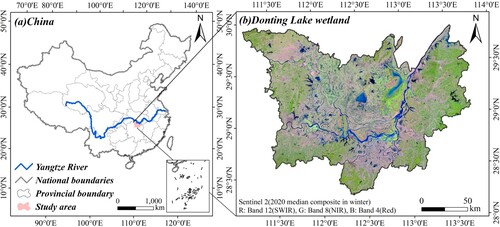
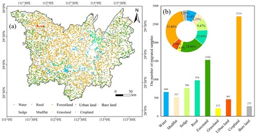
As the second largest freshwater lake in China (2625 km²), Dongting Lake (28°39′–30°14′N, 111°42′–113°39′E) is situated in northern Hunan Province and on the northern side of the Yangtze River (Figure 1). The Dongting Lake wetland is a typical large-scale lake wetland, with significant seasonal changes in hydrology and vegetation (Yang et al. 2020). It features a typical subtropical monsoon climate with dramatic seasonal fluctuation in rainfall, with annual precipitation of approximately 1382 mm (Yang et al. 2020). The wet season of the Dongting Lake wetland generally lasts from April to September (Deng et al. 2014), and the dry season is defined to endure from October to March (Deng et al. 2014). The average annual temperature of this study area ranges from 16.4°C to 17°C (Yang et al. 2020). Moreover, in this study, the spatial extent of Dongting Lake wetland is defined as the boundary of 20 county-level administrative regions involved, with an area of about 2.57 million hectares in total.

Figure 1. (a) Geographical location of the Dongting Lake wetland in China. (b) Sentinel-2 false color image of the Dongting Lake wetland collected and composited in the winter of 2020.

2.2. Dataset and preprocessing

2.2.1 Remote sensing data

In this study, we utilized both Sentinel-1 and Sentinel-2 satellite images (Figure 2) across the study area for annual wetland classification during 2015–2021 within the GEE platform. The total number of level-1 C Sentinel-1 Ground Range Detected images with VV and VH polarizations is 540, of which 534 are ascending tiles. The temporal distribution of the number of Sentinel-1 images from 2016 to 2021 was relatively even, ranging from 70 to 94 (Figure 2), while the number of Sentinel 1 images in 2015 is only 32.

Figure 2. Temporal distribution of Sentinel 1/2 images used in this study. (a) The quantity of Sentinel-1 and Sentinel-2 images used in this study. (b) Scatter plot of Sentinel-2 and Sentinel-1 image acquisition dates in the Dongting Lake wetland during 2015–2021.

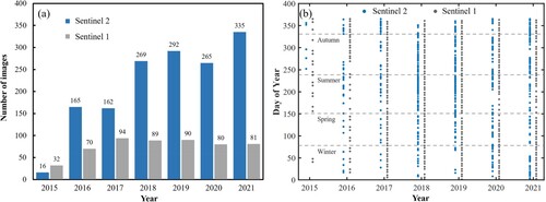
All available Sentinel-2 TOA reflectance data (with cloud cover percentage below 20%) covering the Dongting Lake wetland from 1st January 2015 to 1st January 2022 were obtained through the GEE platform, which totalized to 1504 and accounted for approximately 27.13% of all available images (5543). The yearly and daily distribution of Sentinel imagery’s quantity is shown in Figure. 2. There are few images in 2015, and the number of Sentinel-2 images increased dramatically after 2017. It was obvious that the quantity of images in autumn is more than that in other seasons (Figure 2(b)), partly due to the frequent clouds that occur in summer.

2.2.2 Sample collection in 2020

Referring to Peng et al. (2023), we produced samples for wetland classification in the reference year of 2020 based on an efficient automatic sampling method and manual interpretation by referring to very high-resolution Google Earth images and Normalized Difference Vegetation Index (NDVI) time series. A series of auxiliary datasets (Table A1) were used in this research to assist the generation of large amounts of samples.

First, we extracted the potential distribution extent of wetlands (5 < water occurrence < 85%) and permanent surface water area (water occurrence > 85%) (Zou et al. 2018) based on the Global Surface Water Occurrence (GSWO) dataset (Pekel et al. 2016). Second, using the sampling tool in ArcGIS software, we randomly generated 12,000 sample points across the entire study area to keep the quantity of various nonwetland samples in proportion to area. To ensure that the number of wetland samples was equal to that of nonwetland samples, we generated more wetland samples within the potential distribution extent of wetlands and permanent surface water extent area proportionally. Finally, a total of 13,077 samples were obtained and regarded as the original samples used for future sample migration.

2.3. Refined wetland classification system

Based on the vegetation and hydrological characteristics of DLW, we designed a refined wetland classification scheme (Table 1) suitable for the study area. Except for the traditional wetland categories, we specifically divided the surface water into five subtypes to further distinguish natural and artificial surface water bodies. Although the spatial information of DLW changes greatly in different months within one year due to seasonal variability of rainfall and hydrology, the wetland mapping time in this study is by year since all available satellite data were utilized to characterize various wetland types. It also should be noted that the water cover types in the classification results are generally permanent water.

Table 1. Refined wetland type classification system developed in this study.

Category I	Category II	Description	Sentinel 2 image	Google Earth image	Corresponding class
Natural Wetland	Sedge	Soil moisture is saturated, plant germination time is short, plants are sparse and low lying.
	Reed	It rises up out of the water during floods, but dries out in winter when it covers the banks.
	Mudflat	Includes the floodplain around lakes and rivers.
	Lake	Natural polygonal body of water in inland places with standing water
	River	Natural linear waterbody with flowing water, usually with wandering waterflow
Artificial Wetland	Reservoir	Typically man-made polygonal water featured with standing water and dams
	Ponds	Artificial polygon waterbody with rectangular shape, generally used for aquatic agriculture
	Canal/Channel	Artificial linear waterbody usually with dams or straight boundary
Non-wetland	Cropland	Land for planting crops, including paddy rice
	Forestland	Land where trees, shrubs and other woody plants grow
	Grassland	Land mainly grown with herbaceous plants
	Urban land	Urban and rural residential areas, industrial, mining, transportation land
	Bare land	Dry upland area without vegetation

2.4. Methods

2.4.1 Research framework

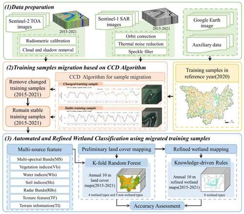
An automatic and refined wetland classification framework which integrates a training sample migration method, supervised machine learning and knowledge-driven decision rules was proposed. It can be divided into the following main sections (Figure 3): (1) Data collection and preparation of Sentinel-1/2 images and auxiliary datasets, (2) Migration of stable training samples in 2020 (reference year) using CCD algorithm, (3) Production of 10 m annual preliminary land cover maps and refined wetland maps (2015-2021) and (4) accuracy assessment.

Figure 3. Schematic flowchart of mapping annual 10 m refined wetlands and other land covers.

2.4.2 Migration of training samples using the continuous change detection algorithm

The CCD algorithm uses a robust method to identify the time when the object changes, and decomposes the time series into two parts: time-invariant and time-varying through maximum likelihood estimation and Markov random field model (Zhu and Woodcock 2014). The CCD was utilized to achieve sample migration, which identifies the samples whose spectral and indicial response patterns have kept unaltered during 2015–2021. Three normalized spectral indices representing the vegetation (NDVI), water inundation (Normalized Difference Water Index, NDWI) and land surface status (Normalized Difference Built-up Index. NDBI) as well as six spectral bands (Red, Green, Blue, Nir, Swir1, Swir2) from time series Sentinel 2 imagery at corresponding location of all reference samples were utilized as input of the CCD algorithm (Jia et al. 2018). The mathematical formulas of CCD algorithm applied for each sample are demonstrated as follows: (1) $\hat{\rho }(i,x{)}_{OLS}=a_{0,i}+a_{1,i}\cos \left({\displaystyle \frac{2\pi }{t}x}\right)+b_{1,i}\sin \left({\displaystyle \frac{2\pi }{t}x}\right)+c_{1,i}x\{{\tau }_{k-1}^{\ast }<x\le {\tau }_k^{\ast }\}$(1) (2) ${\displaystyle \frac{1}{n}\sum _{i=1}^n{\displaystyle \frac{\left|\rho (i,x)-\hat{\rho }{(i,x)}_{OLS}\right|}{3\times RMS{E}_i}}>1\left(\mathrm{T}\mathrm{h}\mathrm{r}\mathrm{e}\mathrm{e}\mathrm{c}\mathrm{o}\mathrm{n}\mathrm{s}\mathrm{e}\mathrm{c}\mathrm{u}\mathrm{t}\mathrm{i}\mathrm{v}\mathrm{e}\mathrm{t}\mathrm{i}\mathrm{m}\mathrm{e}\mathrm{s}\right)}$(2) where i represent the specific spectral reflectance band or feature band, x denotes the date (in Julian format) and t is the total number of days during the study period; $a_{0,i}$ is the overall value of the ith band from a Sentinel-2 image; $a_{1,i}$ and $b_{1,i}$ indicate the intra-annual change; and $c_{1,i}$ stands for interannual changes (Amani et al. 2022); ${\tau }_k^{\ast }$ represents the kth breakpoint; $n$ is the number of all bands(n = 9); $\hat{\rho }(i,x{)}_{OLS}$ and $\rho (i,x)$ is the predicted (based on Ordinary Least Square fitting) and observed value of the ith band at Julian day x, respectively. $RMS{E}_i$ is the root mean square error of the ith band. It should be noted that the CCD algorithm assumes that the phenological changes of stable land cover are consistent. All samples in the reference year were fed into this CCD model to be fitted and regressed based on NDVI, NDWI, NDBI and spectral bands time series. We aim to retrieve the number of breakpoints(k) detected by CCD for all input samples and the algorithm is run using the function ee.Algorithms.TemporalSegmentation.Ccdc() within the GEE platform. If the number of breakpoints for a specific sample is greater than one, it means that the type of this sample has changed during the study period and it would be filtered out. Samples with zero breakpoints would be remained as stable migrated sample for subsequent time series wetland mapping during 2015–2021.

2.4.3 Preliminary land cover classification based on sample migration and random forest model

In this study, we applied the RF classifier (Breiman 2001) to achieve annual preliminary land cover classification using migrated samples obtained in previous step. Considering the complexity and heterogeneity of wetlands, multisource features, including multispectral bands (MS), vegetation indices (VIs), water indices (WIs), soil indices (SIs), radar bands (RBs), texture features (TF) and topographical information (TI), were utilized for wetland classification. To fully extract the intra-annual phenological and hydrological time series features from Sentinel imagery, which is critical for delineating wetlands (Kool et al. 2022), we aggregated time series satellite images into phenology-based features in the GEE platform(Jia et al. 2020; Peng et al. 2023; Wang et al. 2022). First, we composited Sentinel 2 images into the wettest images and the greenest images through the ‘qualityMosaic’ function (Jia et al. 2020). Second, we also utilized multiple percentile (10%, 20%, 30%, 40%, 50%, 60%, 70%, 80%, 90%) features by composite time series images using ee.Reducer.percentile()” function and statistical features (including median, maximum, minimum, and standard deviation) of MS, VIs, WIs and SIs as input features. The TF included 8 textual features from gray-level co-occurrence matrix of the maximum NDVI. The TI comprises DEM, slope and aspect features. The RBs are two median composites of VV and VH polarization channel from Sentinel 1 images in each year. Detailed descriptions of these features are shown in Table A2. Finally, a total of 189 feature variables in each year during 2015–2021 were fed into the 10-fold RF model and the majority of the resultant 10 classification results were taken as the final land cover type for each 10 m pixel(Peng et al. 2023).

2.4.4 Refined wetland mapping based on knowledge-driven decision rules

Based on water cover’s geometric features and available water-related inventories, we designed a knowledge-guided hierarchical decision-rule method to separate rivers, lakes, reservoirs, ponds and canals/channels and thus achieve refined wetland mapping. The overall flowchart of this method is illustrated in Figure 4 and includes five steps:

1. Based on the surface water body raster map reclassified from the preliminary land cover maps, we generated corresponding surface water body vector maps in each year during 2015–2021. Then, they were reprojected to the Krasovsky_1940_Albers equal area projection (Wang, Xiao, et al. 2022), and the area (ha) of each polygon was calculated. Considering that the number of spatial combinations of water polygons with few pixels are limited, water polygons with area less than 1ha were directly labeled as small ponds and the rest water polygons were retained for subsequent classification.

2. Points of interest (POIs) of reservoirs from Gaode map (https://lbs.amap.com/) were utilized to identify reservoirs by intersecting with water polygons with a 200 m buffer (to avoid trivial deviation). To prevent overinclusion of small water patches (i.e. ponds) surrounding large lakes, we first generated the centroid of lakes from related lake datasets (Table A1) and selected water polygons overlaying with these centroids as large lake polygons.

3. Using open-access and advanced geospatial data analysis tools (Lindsay et al., 2014)-WhiteboxTools v2.0 (https://github.com/giswqs/WhiteboxTools-ArcGIS), we calculated the Compactness, Shape Complexity Index and Linearity Index (Table 2) for all water polygons. After trial and experiments, we optimized the thresholds of shape-based features (Figure 5) and design discrimination rules (Figure 4) to separate rivers, ponds, and canals/channels.

Figure 4. Flowchart of the method proposed for identifying multitype water covers, including rivers, lakes, reservoirs, ponds and canals/channels.

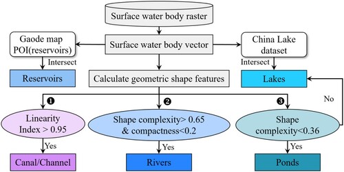
Figure 5. Shape complexity index, Linearity Index and Compactness for different water types.

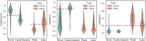
Table 2. The geometric shape features used in the study.

Name	Description		Calculation formula	Variable Definitions	Schematic illustration of indices (McGlone, D., 2016)
Compactness (Polsby-Popper index)	It is the polygon area divided by the district to the area of a circle with a perimeter equal to the that of the polygon.		${\displaystyle \frac{4\pi A}{P^2}}$	Where A is the polygon's area and P is the perimeter of the polygon
Shape Complexity Index	It is designed for measuring the complexity of a vector polygon, which is also independent of its elongation.		$1-{\displaystyle \frac{A}{A_h}}$	Where A, Ah is the area of the polygon and the convex hull containing the polygon, respectively.
Linearity Index	It is the determinant coefficient (R^2) from the regression of the x and y coordinates value of the convex hull nodes of a polygon.		-	-

2.4.5 Accuracy assessment

In this study, 20% of the migrated samples were randomly selected to assess the performance of preliminary land cover results. Additionally, a set of independent third-party samples (seen in Table A4), visually interpreted by combining historical high-resolution images in Google Earth and indices time series on Collect Earth, were utilized assess the accuracy of the refined wetland maps. The accuracy assessment is performed by computing a confusion matrix and calculating the overall accuracy (OA), kappa coefficient, user accuracy (UA) and producer accuracy (PA)(Mao et al. 2020; Zhang et al. 2023). We also calculated the F₁ scores to the PA and UA and better described the classification accuracy for various wetland covers. Additionally, we compared our results against other publicly available land cover and water-related products to verify the reliability of wetland maps obtained more comprehensively.

3. Results

3.1. Migrated training samples using continuous change detection algorithm

We finally identified 8112 unchanged samples from 13,077 reference samples in the DLW, and the spatial distribution of these unchanged samples is shown in Figure 6(a). The number of each wetland or land cover class is illustrated in Figure 6(b). The quantity of migrated samples for cropland cover is the largest, followed by forestland, water and reed. Generally, the quantity and spatial distribution of various land cover samples are even and proportional to their extent. These nine-type migrated land cover samples are divided into training samples and testing samples by a ratio of 4:1 and the corresponding number could be seen in Table A4.

Figure 6. (a) The spatial distribution of the migrated unchanged training sample. (b) The number of migrated samples in each land cover type in DLW.

Additionally, we randomly selected 50 migrated samples for each land cover type and interpreted if them have changed during 2015–2021 via Google Earth history very high-resolution images. To avoid random subjective errors caused by various reorganizations, we asked three interpreters with rich professional experience to make judgements about whether each sample changed during the period and adopt the result where at least two people agree. The results denote that the overall accuracy of migrated samples for all land cover are all above 98% (shown in Table A5), demonstrating high potential of sample migration by using CCD algorithm.

3.2. Annual maps of preliminary land cover from 2015 to 2021 and accuracy assessment

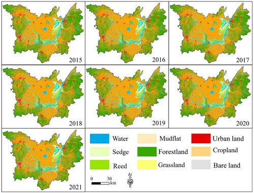
The annual 10 m preliminary land cover maps during 2015–2021 in the DLW are shown in Figure 7, which include 4 coarse wetland types and 5 nonwetland types. It could be seen that wetlands were mainly located around Dongting Lake and surrounding river networks, with a layer-by-layer distribution characteristic around the permanent surface water. Intuitively, the spatial changes in wetlands over the past seven years were scarce, partly due to the limited temporal period and enhanced protection policies.

Figure 7. The annual land cover maps of DLW during 2015–2020.

Additionally, the accuracy assessment results are demonstrated in Table 3. The OA of preliminary land cover classification was all above 83% and ranged from 83.59% (2015) to 89.46% (2020), with the Kappa coefficients varying from 0.80 in 2015 to 0.87 in 2020. For all wetland classes, the OAs in each year from 2015 to 2021 reached above 86%, with the highest in 2020 (94.18%), possibly due to more sufficient samples for classification. The averaged F₁ scores of water, mudflat, sedge, reed, forestland and grassland during 2017–2021 were above 0.85, while cropland and bareland’s F₁ scores were 0.84 and 0.72 on average, respectively.

Table 3. The accuracy of wetland and nonwetland cover classification during 2015–2021.

		Water	Mudflat	Sedge	Reed	Forestland	Grassland	Urban land	Cropland	Bare land	OA (all)	KC	OA (wetland)
2015	PA(%)	93.55	96.26	75.9	85.14	81.19	92.16	71.76	84.34	68.18	83.59%	0.80	86.06%
	UA(%)	93.55	96.26	86.3	75.63	84.54	90.38	83.56	79.23	93.75
	F1	0.94	0.96	0.81	0.80	0.83	0.91	0.77	0.82	0.79
2016	PA(%)	95.97	99.07	78.31	89.71	77.96	92.59	75.86	89.82	57.89	85.95%	0.83	88.89%
	UA(%)	93.7	93.81	90.28	85.79	89.77	100	84.62	79.27	78.57
	F1	0.95	0.96	0.84	0.88	0.83	0.96	0.80	0.84	0.67
2017	PA(%)	97.58	98.13	78.31	89.14	82.51	94.12	82.35	86.69	63.64	86.27%	0.83	89.52%
	UA(%)	93.08	97.22	87.84	82.11	90.25	96.00	86.42	80.69	84.85
	F1	0.95	0.98	0.83	0.85	0.86	0.95	0.84	0.84	0.73
2018	PA(%)	96.77	95.33	74.55	90.29	82.51	92.16	81.93	88.21	75.51	86.46%	0.83	87.35%
	UA(%)	91.6	94.44	87.86	80.61	91.24	92.16	87.18	82.23	88.1
	F1	0.94	0.95	0.81	0.85	0.87	0.92	0.84	0.85	0.81
2019	PA(%)	97.58	96.26	86.75	92.57	85.48	90.20	80.00	84.74	63.64	87.10%	0.84	90.14%
	UA(%)	91.67	96.26	91.14	84.82	88.1	95.83	80.00	84.24	75.68
	F1	0.95	0.96	0.89	0.89	0.87	0.93	0.80	0.84	0.69
2020	PA(%)	99.19	99.07	96.99	91.43	85.1	88.24	83.75	86.69	77.55	89.46%	0.87	94.18%
	UA(%)	96.09	97.25	92.00	93.02	90.81	97.83	87.01	85.52	66.67
	F1	0.98	0.98	0.94	0.92	0.88	0.93	0.85	0.86	0.72
2021	PA(%)	98.39	99.07	93.37	84.00	82.84	84.31	79.76	88.45	64.44	87.61%	0.85	90.60%
	UA(%)	96.06	96.36	88.07	85.47	94.36	95.56	83.75	82.78	65.91
	F1	0.97	0.98	0.91	0.85	0.88	0.90	0.82	0.86	0.65

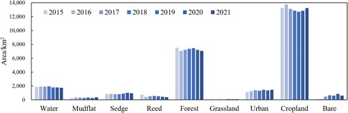
The temporal changes of various land cover types’ areas in the DLW are depicted in Figure 8. Overall, the temporal changes in the four wetland covers were not very significant. The area of water declined by approximately 5.93%, from 1851.47 km² in 2015 to 1741.76 km² in 2021, and the area of reeds decreased from 742.57 to 388.8 km² from 2015 to 2021. The extent of mudflats and sedges presented a fluctuating increasing trend in the last seven years, with 98.43 and 104.68 km^2, respectively. The total area of wetlands decreased slightly by 4.87% during the same period, from 3709.09 to 3448.72 km².

Figure 8. The area of wetlands and nonwetland covers during 2015-2021.

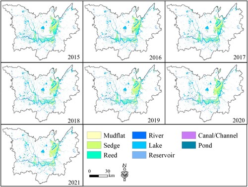
3.3. Annual maps of refined wetlands from 2015 to 2021 and accuracy assessment

On the basis of the preliminary land cover classification results generated above, we achieved continuous annual 10 m refined wetland mapping in the DLW from 2015 to 2021 (Figure 9), with a total of 8 wetland types. We can see that the mudflats and reeds in the DLW are distributed around the center of the lake and the river system, showing a spatial pattern of concentric circles and intermixed distribution.

Figure 9. The annual refined wetland maps of DLW during 2015–2020.

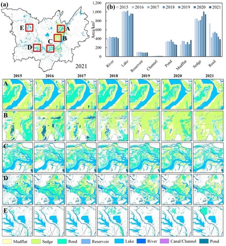
The spatial details of refined wetland results for five typical sites in the DLW are illustrated in Figure 10(a). Generally, the area of reed, lake and pond presented an overall downward trend during recent 7 years, while the area of sedge had grown. The area of river, reservoir, channel and mudflat remained slightly fluctuant around 428.18, 95.67, 14.20 and 317.11 km² on average, respectively (Figure 10(b)).

Figure 10. (a)Spatial details of annual refined wetland maps from 2015 to 2021 for five typical sites(A-E) in the DLW and (b) the temporal changes of various wetland area.

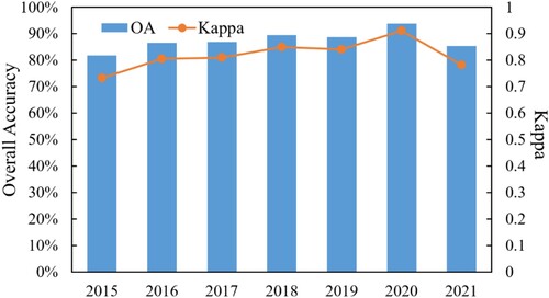
The OA and kappa coefficient for the resultant refined wetland maps are shown in Figure 11. It can be clearly seen that the overall accuracies are all above 80%, with the highest in 2020 the lowest in 2015 (81.82%), mainly due to a lack of images.

Figure 11. The accuracy of refined wetland maps in DLW during 2015–2021.

3.4. Intercomparison between wetlands in this study and existing products

3.4.1 Comparison with other LULC products

To further validate the accuracy of the wetland maps in this study, three Land Use Land Cover (LULC) data products with 10 m or higher resolution were selected and four typical sites around the Dongting Lake were chosen to illustrate the intercomparison results (Figure 12). The ESA WorldCover 2020 is a global land cover product with a 10 m resolution produced from Sentinel-1 and Sentinel-2 data, of which the wetland classes include permanent water bodies and herbaceous wetlands. Dynamic World (Brown et al. 2022) is a near real-time global 10 m land cover dataset generated from deep learning using Sentinel-2 imagery, we utilized the land cover map in 2020 composited by majority voting within the GEE platform, of which flooded vegetation and water were selected for comparison. The CECD data product is a land cover dataset produced by the Ministry of Ecology and Environment of China via visual interpretation, with a 5 m spatial resolution in 2020 and detailed wetland types.

Figure 12. Comparison between various LULC datasets and the wetland maps in this study over the DLW.

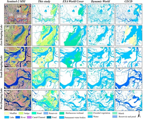
Given the disparity between these products’ classification system and our results, we reclassify and put our focus on wetland types. It is noticeable that the wetland categories in this study are more detailed than those in other LULC datasets. Additionally, the spatial details of wetlands in this study are more abundant. These illustrations in three typical wetlands (East, South and West Dongting Lake) show the advantages of our wetland maps in both spatial details and types.

3.4.2 Comparison with water-related products

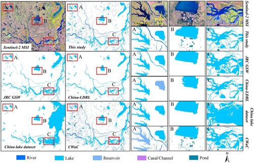
Furthermore, we selected four water-related thematic datasets to verify the accuracy as well via intercomparison between water cover results in this study with the JRC Global Surface Water (GSW) (Pekel et al. 2016), China-LDRL dataset (Wang et al., 2022b), China Lake dataset (1960s-2020) (Zhang et al., 2019) and CWaC (2020/10 m) (Li and Niu 2022). To facilitate the comparison, we extracted GSW permanent surface water in 2020 based on index-based thresholding method (Deng et al., 2019; Deng et al., 2022). The China-LDRL dataset is a vector map of surface water bodies, large dams, reservoirs and lakes (surface water area > 1 km²) in China in 2019, and the China Lake dataset includes lakes (area > 1 km²) during 1960–2020. We mainly compared the reservoirs and lakes with that in these datasets. The CWaC was chosen to compare rivers, reservoirs, lakes, and ponds with our results. As is illustrated in Figure 13, Shanpo Lake was misclassified as a reservoir in China-LDLR, and Maoli Lake was misidentified as a reservoir in CWaC. In addition, our results and CwaC showed more spatial details about ponds. Generally, the water cover results in this study present more information about wetland types and spatial details, which could make up for the lack of existing products to a certain extent and provide data support for water-type wetland monitoring and conservation.

Figure 13. Comparison between various water-related products in 2020 over the DLW, with three close-up maps located in lakes, ponds and rivers.

4. Discussion

4.1 Advantages in the automated and refined wetland mapping algorithm

In this study, we proposed an automatic and refined wetland mapping method which combines sample migration and hierarchical decision rule to improve the timeliness and information richness of wetland mapping in lacustrine wetlands with abundant wetland types. Compared with previous studies (Ghorbanian et al. 2020; Zhu et al., 2021), we have improved the continuous wetland mapping framework in three aspects: (1) we applied the CCD algorithm into training sample migration, which is more intelligent and robust since it could effectively capture the inter and intra-annual change patterns for various land covers; (2) the multitype water-type wetlands obtained in this study give richer categorical information, which could support refined conservation for wetland ecosystems; (3) the employment of the GEE platform and open source geospatial tools enable the methodological framework more operational and has great potential for practical applications elsewhere.

Moreover, compared with deep learning algorithms used in wetland vegetation mapping and monitoring, which shows advantages of state-of-the-art performance, automatic feature learning, adaptability and scalability and so on, the automated and refined wetland classification method developed in this study are mainly based on traditional machine learning and decision rules, which could lack advantages in classification accuracy when applied in complex tasks. However, deep learning methods possibly have disadvantages of ‘black-box’ issues, overfitting tendencies, requirements of large amount of data and costly computing resources, which could be difficult for users to achieve in certain circumstances, while the developed wetland classification framework is relatively easier to comprehend and operated for its utilization of GEE platform and lower sample requirements.

4.2. Limitations and future improvements

Although the results have demonstrated good performance and potential of the proposed automated and refined wetland mapping framework, there still remain some limitations. First, it was found that a substantial number of detected changed samples were abandoned after sample migration, which possibly decreased the mapping accuracy. Therefore, it is suggested that as many samples as possible interpreted in the reference year, collected from other years or similar regions be generated to promote the classification accuracy. It should also be noted that some inherent errors in reference samples have direct impacts on the mapping accuracy (Ghorbanian et al. 2020). Second, the Sentinel-2 time series leveraged might be contaminated by cloud or cloud shadow, which commonly occurs in subtropical areas, therefore decreasing the classification accuracy. To address this problem, some spatiotemporal fusion algorithms could be utilized to reconstruct missing values, although this process requires much more workload. Third, the selection of threshold values for distinguishing water types still remains slightly uncertain if applied in other areas with different terrain or landforms conditions. Therefore, the constructed ruleset should be applied in other regions to investigate universality. In addition, under some particular circumstances, lakes and rivers were connected together and formed a whole water polygon, leading to some errors in classification results, thus a few manual corrections and post-processing are needed.

Due to the main purpose of this study is to verify the feasibility and accuracy of the proposed wetland mapping framework, a typical lake wetland with a rich variety of wetland types was selected for demonstration. In the future, this method will be extended to other typical wetland areas and compared with more advanced machine learning algorithms to further examine the feasibility of the wetland classification framework using migrated samples.

5. Conclusions

Using temporally dense Sentinel-1/2 imagery during 2015–2021, this study proposed an automated and refined wetland mapping framework integrating a sample migration method, supervised machine learning and knowledge-driven decision rules to investigate the wetland dynamics and facilitate decision-making of wetland conservation. Annual 10 m refined wetland maps of DLW from 2015 to 2021 were obtained accurately and efficiently, with OA reaching above 86% each year, which indicates the superiority of the methodology. The total area of the DLW showed a slight downward trend from 3709.11 km² in 2015 to 3448.73 km² in 2021.

Overall, the timeliness and efficiency of this automatic and refined wetland mapping framework proposed enable us to achieve up-to-date accurate wetland mapping cost-effectively and this framework could provide potential methodological references in other regions of interest. The resultant refined wetland maps are able to provide timely and effective support for decision-making related to wetland conservation and management as well as promoting regional sustainable development, especially for areas where historical training samples are difficult and costly to obtain.

Acknowledgements

We also thank the anonymous reviewers for their helpful comments.

Disclosure statement

No potential conflict of interest was reported by the author(s).

Data availability statement

The data that support the findings of this study are available from the corresponding author, upon reasonable request.

Additional information

Funding

The work was jointly supported by the National Natural Science Foundation of China (grant numbers 42071393, U1901219 and U21A2022).

Appendix

Table A1. Auxiliary datasets used in this research.

Name of dataset	Time	Resolution	Purpose in this study	Data Source
Global Surface Water (GSW)	1984–2021	30 m	Identify water and potential wetlands extent	https://global-surface-water.appspot.com
China lake dataset (CLD)	1960s–2020	vector	Identify lake	https://data.tpdc.ac.cn/zh-hans/disallow/fa8426c0-d3f0-4615-8e78-0465a0957891/
China’s Large Dams, Reservoirs and Lakes(China-LDRL)	2019	30 m/vector	Identify reservoir and lake	https://figshare.com/articles/dataset/China-LDRL_dataset/16964656/3
China Water Cover Map (CwaC) dataset	2020	10 m	Identify river, reservoir, lake and pond	http://www.doi.org/10.11922/sciencedb.00880
Global River Widths from Landsat (GRWL)		Vector	Identify rivers	https://zenodo.org/record/1297434#.Yw2v2XZBy3C
Gaode map Points of Interest (reservoirs)	/	Points	Identify reservoir	https://lbs.amap.com/api/webservice/guide/api/search
ESA WorldCover	2020	10 m	Generating samples	https://esa-worldcover.org/en
China Land Cover Database (CLCD)	2020	30 m	Generating samples	https://zenodo.org/record/5816591#.Yww9YXZBy3A
China Land Use Database (CLUD)	2020	30 m	Generating samples	https://www.resdc.cn/
Global Land-cover Product with Fine Classification System at 30 m (GLC_FCS30)	2020	30 m	Generating samples	https://zenodo.org/record/4280923#.YwtJCXZBy3A

Table A2. Multi-source features used for wetland classification in this study.

Feature type	Feature name	Description	GEE calculation code	Number of features
Multi-spectral bands (MS)	B2∼B8, B8A, B11∼12	Spectral reflectance in various band	select(["B2", "B3", "B4", "B5", "B6", "B7","B8", "B8A", "B11", "B12"]	20
Vegetation indices (VIs)	NDVI	Normalized Difference Vegetation Index	normalizedDifference(['B8', 'B4'])	91
	EVI	Enhanced Difference Vegetation Index	2.5 * ((NIR−Red) / (NIR + 6 * Red−7.5 * Blue + 1))
	SAVI	Soil-Adjusted Vegetation Index	(((SWIR−R) / (SWIR + R + 0.5)) * 1.5)−(SWIR2 / 2)
	PSRI	Plant Senescence Reflectance Index	(B4−B2) / B5
	ARI	Anthocyanin Reflectance Index	(B8 / B2)−(B8 / B3)
	REIP	Red edge inflection point	705 + 35*((((RED + RE3)/2)−RE1) / (RE2−RE1))
	IRECI	Inverted red-edge chlorophyll index	(NIR–RED) / (RE1/RE2)
Water indices (WIs)	NDWI	Normalized difference water index	normalizedDifference(['B3', 'B8'])	39
	MNDWI	Modified Normalized Difference Water Index	normalizedDifference(["B3", "B11"])
	LSWI	Land Surface Water Index	normalizedDifference(["B8","B11"])
Soil indices (SIs)	BSI	Bare Soil Index	((SWIR1+red)-(NIR+blue))/((SWIR1+red)+(NIR+blue))	26
	NDBI	Normalized Difference Built-up Index	normalizedDifference(['B12', 'B8'])
Radar Bands (RBs)	VV	VV polarization	select(["VV"])	2
	VH	VH polarization	select(["VH"])
Texture feature (TF)	GLCM indices	Gray-Level Co-occurrence Matrix indices:"mean","variance","homogeneity", "contrast","dissimilarity","entropy", "second_moment","correlation"	NDVI.glcmTexture().select(['ndvi_idm', 'ndvi_diss', 'ndvi_contrast', 'ndvi_ent', 'ndvi_asm', 'ndvi_savg', 'ndvi_var', 'ndvi_corr']);	8
Height information (DEM)	DEM	STRM DEM	ee.Image('USGS/SRTMGL1_003')	3
	Slope	Slope	ee.Terrain.slope(DEM)
	Aspect	Aspect	ee.Terrain.aspect(DEM)

Table A3. The area of wetlands in Dongting Lake Wetland during 2015∼2021(unit:km²).

	Category	2015	2016	2017	2018	2019	2020	2021
Natural wetland	Mudflat	271.22	353.00	346.47	275.30	326.19	277.93	369.65
	Sedge	843.84	851.84	803.96	818.46	903.78	1009.17	948.51
	Reed	742.57	433.22	529.86	554.02	521.34	446.08	388.80
	River	404.50	445.13	431.66	438.35	428.47	438.24	410.94
	Lake	1005.22	1018.20	1001.34	1026.58	918.15	966.14	956.71
Artificial wetland	Reservoir	100.92	103.34	104.41	93.97	86.24	87.74	93.08
	Canal/Channel	8.17	13.51	16.41	14.19	17.70	14.58	14.85
	Pond	332.67	347.94	339.93	375.33	329.35	278.71	266.19
Non-wetland	Forestland	7517.71	7070.49	7221.69	7364.64	7445.32	7185.51	7060.36
	Grassland	81.27	45.34	58.68	45.20	101.47	78.86	80.04
	Urban land	1118.79	1250.35	1407.69	1304.90	1442.74	1346.67	1447.92
	Cropland	13232.21	13746.75	13098.49	12862.45	12687.87	12828.68	13207.92
	Bare land	163.56	143.51	462.05	649.25	614.00	864.32	598.33

Table A4. The number of samples used for Dongting Lake Wetland classification during 2015–2021.

		Training samples	Testing samples
	Category	2015–2021	2015	2016	2017	2018	2019	2020	2021
Natural wetland	Mudflat	410	107	107	107	107	107	107	107
	Sedge	602	166	166	166	166	166	166	166
	Reed	801	175	175	175	175	175	175	175
	River	536(Water)	69	69	69	69	68	68	67
	Lake		136	136	136	136	136	136	136
Artificial wetland	Reservoir		35	35	35	35	35	35	35
	Canal/Channel		19	19	19	19	18	16	13
	Pond		38	38	38	38	37	37	35
Non-wetland	Forestland	1226	304	304	304	304	304	304	304
	Grassland	162	51	51	51	51	51	51	51
	Urban land	376	85	85	85	85	85	85	85
	Cropland	2203	511	511	511	511	511	511	511
	Bare land	229	44	44	44	44	44	44	44

Table A5. The number of righteous migrated samples from 50 samples randomly selected for nine land cover types.

Category	Unchanged	Changed	Accuracy
Mudflat	49	1	98%
Sedge	49	1	98%
Reed	49	1	98%
Water	50	0	100%
Forestland	50	0	100%
Grassland	49	1	98%
Urban land	50	0	100%
Cropland	50	1	98%
Bare land	49	1	98%

References

- Allen, George H., and Tamlin M. Pavelsky. 2018. “Global Extent of Rivers and Streams.” Science 361 (6402): 585–588. https://doi.org/10.1126/science.aat0636.
- Amani, Meisam, Mohammad Kakooei, Arsalan Ghorbanian, Rebecca Warren, Sahel Mahdavi, Brian Brisco, Armin Moghimi, et al. 2022. “Forty Years of Wetland Status and Trends Analyses in the Great Lakes Using Landsat Archive Imagery and Google Earth Engine.” Remote Sensing 14. https://doi.org/10.3390/rs14153778.
- Belgiu, Mariana, and Lucian Drăguţ. 2016. “Random Forest in Remote Sensing: A Review of Applications and Future Directions.” ISPRS Journal of Photogrammetry and Remote Sensing 114: 24–31. https://doi.org/10.1016/j.isprsjprs.2016.01.011.
- Berhane, T. M., C. R. Lane, Q. Wu, B. C. Autrey, O. A. Anenkhonov, V. V. Chepinoga, and H. Liu. 2018. “Decision-Tree, Rule-Based, and Random Forest Classification of High-Resolution Multispectral Imagery for Wetland Mapping and Inventory.” Remote Sensing 10 (4): 580. https://doi.org/10.3390/rs10040580.
- Breiman, Leo. 2001. “Random Forests.” Machine Learning 45 (1): 5–32. https://doi.org/10.1023/A:1010933404324.
- Brown, Christopher F., Steven P. Brumby, Brookie Guzder-Williams, Tanya Birch, Samantha Brooks Hyde, Joseph Mazzariello, Wanda Czerwinski, et al. 2022. “Dynamic World, Near Real-Time Global 10 m Land use Land Cover Mapping.” Scientific Data 9 (1), https://doi.org/10.1038/s41597-022-01307-4.
- Cai, Yaotong, Xinyu Li, Meng Zhang, and Hui Lin. 2020. “Mapping Wetland Using the Object-Based Stacked Generalization Method Based on Multi-Temporal Optical and SAR Data.” International Journal of Applied Earth Observation and Geoinformation 92. https://doi.org/10.1016/j.jag.2020.102164.
- Debanshi, Sandipta, and Swades Pal. 2020. “Wetland Delineation Simulation and Prediction in Deltaic Landscape.” Ecological Indicators 108. https://doi.org/10.1016/j.ecolind.2019.105757.
- Deng, Yue, Weiguo Jiang, Zhenghong Tang, Ziyan Ling, and Zhifeng Wu. 2019. “Long-term changes of open-surface water bodies in the Yangtze River basin based on the Google Earth Engine cloud platform.” Remote Sensing 11 (19): 2213.
- Deng, Yawen, Weiguo Jiang, Zhifeng Wu, Ziyan Ling, Kaifeng Peng, and Yue Deng. 2022. “Assessing surface water losses and gains under rapid urbanization for SDG 6.6. 1 using long-term Landsat imagery in the Guangdong-Hong Kong-Macao Greater Bay Area, China.” Remote Sensing 14 (4): 881.
- Deng, Fan, Xuelei Wang, Xiaobin Cai, Enhua Li, Liuzhi Jiang, Hui Li, and Ranran Yan. 2014. “Analysis of the Relationship Between Inundation Frequency and Wetland Vegetation in Dongting Lake Using Remote Sensing Data.” Ecohydrology 7 (2): 717–726. https://doi.org/10.1002/eco.1393.
- Fekri, Erfan, Hooman Latifi, Meisam Amani, and Abdolkarim Zobeidinezhad. 2021. “A Training Sample Migration Method for Wetland Mapping and Monitoring Using Sentinel Data in Google Earth Engine.” Remote Sensing 13 (20), https://doi.org/10.3390/rs13204169.
- Fu, Bolin, Feiwu Lan, Hang Yao, Jiaoling Qin, Hongchang He, Lilong Liu, Liangke Huang, Dongling Fan, and Ertao Gao. 2022. “Spatio-temporal Monitoring of Marsh Vegetation Phenology and its Response to Hydro-Meteorological Factors Using CCDC Algorithm with Optical and SAR Images: In Case of Honghe National Nature Reserve, China.” Science of The Total Environment 843: 156990. https://doi.org/10.1016/j.scitotenv.2022.156990.
- Gallant, Alisa. 2015. “The Challenges of Remote Monitoring of Wetlands.” Remote Sensing 7 (8): 10938–10950. https://doi.org/10.3390/rs70810938.
- Ghorbanian, Arsalan, Mohammad Kakooei, Meisam Amani, Sahel Mahdavi, Ali Mohammadzadeh, and Mahdi Hasanlou. 2020. “Improved Land Cover map of Iran Using Sentinel Imagery Within Google Earth Engine and a Novel Automatic Workflow for Land Cover Classification Using Migrated Training Samples.” ISPRS Journal of Photogrammetry and Remote Sensing 167: 276–288. https://doi.org/10.1016/j.isprsjprs.2020.07.013.
- Gorelick, Noel, Matt Hancher, Mike Dixon, Simon Ilyushchenko, David Thau, and Rebecca Moore. 2017. “Google Earth Engine: Planetary-Scale Geospatial Analysis for Everyone.” Remote Sensing of Environment 202: 18–27. https://doi.org/10.1016/j.rse.2017.06.031.
- Han, Xingxing, Xiaoling Chen, and Lian Feng. 2015. “Four Decades of Winter Wetland Changes in Poyang Lake Based on Landsat Observations Between 1973 and 2013.” Remote Sensing of Environment 156: 426–437. https://doi.org/10.1016/j.rse.2014.10.003.
- Hu, S., Z. Niu, Y. Chen, L. Li, and H. Zhang. 2017. “Global Wetlands: Potential Distribution, Wetland Loss, and Status.” Science of The Total Environment 586: 319–327. https://doi.org/10.1016/j.scitotenv.2017.02.001.
- Huang, Huabing, Jie Wang, Caixia Liu, Lu Liang, Congcong Li, and Peng Gong. 2020. “The Migration of Training Samples Towards Dynamic Global Land Cover Mapping.” ISPRS Journal of Photogrammetry and Remote Sensing 161: 27–36. doi:https://doi.org/10.1016/j.isprsjprs.2020.01.010.
- Jahncke, Raymond, Brigitte Leblon, Peter Bush, and Armand LaRocque. 2018. “Mapping Wetlands in Nova Scotia with Multi-Beam RADARSAT-2 Polarimetric SAR, Optical Satellite Imagery, and Lidar Data.” International Journal of Applied Earth Observation and Geoinformation 68: 139–156. doi:https://doi.org/10.1016/j.jag.2018.01.012.
- Jia, Kai, Weiguo Jiang, Jing Li, and Zhenghong Tang. 2018. “Spectral Matching Based on Discrete Particle Swarm Optimization: A new Method for Terrestrial Water Body Extraction Using Multi-Temporal Landsat 8 Images.” Remote Sensing of Environment 209: 1–18. doi:https://doi.org/10.1016/j.rse.2018.02.012.
- Jia, Mingming, Dehua Mao, Zongming Wang, Chunying Ren, Qiande Zhu, Xuechun Li, and Yuanzhi Zhang. 2020. “Tracking Long-Term Floodplain Wetland Changes: A Case Study in the China Side of the Amur River Basin.” International Journal of Applied Earth Observation and Geoinformation 92), https://doi.org/10.1016/j.jag.2020.102185.
- Jia, Mingming, Zongming Wang, Dehua Mao, Chunying Ren, Chao Wang, and Yeqiao Wang. 2021. “Rapid, Robust, and Automated Mapping of Tidal Flats in China Using Time Series Sentinel-2 Images and Google Earth Engine.” Remote Sensing of Environment. https://doi.org/10.1016/j.rse.2021.112285.
- Kool, Juliette, Stef Lhermitte, Markus Hrachowitz, Francesco Bregoli, and Michael E. McClain. 2022. “Seasonal Inundation Dynamics and Water Balance of the Mara Wetland, Tanzania Based on Multi-Temporal Sentinel-2 Image Classification.” International Journal of Applied Earth Observation and Geoinformation 109: 102766. https://doi.org/10.1016/j.jag.2022.102766.
- Li, Yang, and Zhenguo Niu. 2022. “Systematic Method for Mapping Fine-Resolution Water Cover Types in China Based on Time Series Sentinel-1 and 2 Images.” International Journal of Applied Earth Observation and Geoinformation 106. https://doi.org/10.1016/j.jag.2021.102656.
- Lindsay, J. B. 2014. The whitebox geospatial analysis tools project and open-access GIS. Paper presented at the Proceedings of the GIS Research UK 22nd Annual Conference, The University of Glasgow.
- Liu, Jiyuan, Wenhui Kuang, Zengxiang Zhang, Xinliang Xu, Yuanwei Qin, Jia Ning, Wancun Zhou, et al. 2014. “Spatiotemporal Characteristics, Patterns, and Causes of Land-use Changes in China Since the Late 1980s.” Journal of Geographical Sciences 24 (2): 195–210. https://doi.org/10.1007/s11442-014-1082-6.
- Liu, Yang, Huaiqing Zhang, Meng Zhang, Zeyu Cui, Kexin Lei, Jing Zhang, Tingdong Yang, and Ping Ji. 2022. “Vietnam Wetland Cover map: Using Hydro-Periods Sentinel-2 Images and Google Earth Engine to Explore the Mapping Method of Tropical Wetland.” International Journal of Applied Earth Observation and Geoinformation 115. https://doi.org/10.1016/j.jag.2022.103122.
- Mao, Dehua, Zongming Wang, Baojia Du, Lin Li, Yanlin Tian, Mingming Jia, Yuan Zeng, Kaishan Song, Ming Jiang, and Yeqiao Wang. 2020. “National Wetland Mapping in China: A new Product Resulting from Object-Based and Hierarchical Classification of Landsat 8 OLI Images.” ISPRS Journal of Photogrammetry and Remote Sensing 164: 11–25. https://doi.org/10.1016/j.isprsjprs.2020.03.020.
- Mao, Dehua, Zongming Wang, Jianguo Wu, Bingfang Wu, Yuan Zeng, Kaishan Song, Kunpeng Yi, and Ling Luo. 2018. “China's Wetlands Loss to Urban Expansion.” Land Degradation & Development 29 (8): 2644–2657. https://doi.org/10.1002/ldr.2939.
- Maxwell, Aaron E., Timothy A. Warner, and Fang Fang. 2018. “Implementation of Machine-Learning Classification in Remote Sensing: An Applied Review.” International Journal of Remote Sensing 39 (9): 2784–2817. https://doi.org/10.1080/01431161.2018.1433343.
- Messager, M. L., B. Lehner, G. Grill, I. Nedeva, and O. Schmitt. 2016. “Estimating the Volume and age of Water Stored in Global Lakes Using a geo-Statistical Approach.” Nature Communications 7: 13603. https://doi.org/10.1038/ncomms13603.
- Pekel, J. F., A. Cottam, N. Gorelick, and A. S. Belward. 2016. “High-resolution Mapping of Global Surface Water and its Long-Term Changes.” Nature 540 (7633): 418–422. https://doi.org/10.1038/nature20584.
- Peng, Kaifeng, Weiguo Jiang, Peng Hou, Zhifeng Wu, Ziyan Ling, Xiaoya Wang, Zhenguo Niu, and Dehua Mao. 2023. “Continental-scale Wetland Mapping: A Novel Algorithm for Detailed Wetland Types Classification Based on Time Series Sentinel-1/2 Images.” Ecological Indicators 148. https://doi.org/10.1016/j.ecolind.2023.110113.
- Radoux, Julien, Céline Lamarche, Eric Bogaert, Sophie Bontemps, Carsten Brockmann, and Pierre Defourny. 2014. “Automated Training Sample Extraction for Global Land Cover Mapping.” Remote Sensing 6: 3965–3987. https://doi.org/10.3390/rs6053965.
- Slagter, Bart, Nandin-Erdene Tsendbazar, Andreas Vollrath, and Johannes Reiche. 2020. “Mapping Wetland Characteristics Using Temporally Dense Sentinel-1 and Sentinel-2 Data: A Case Study in the St. Lucia Wetlands, South Africa.” International Journal of Applied Earth Observation and Geoinformation 86. https://doi.org/10.1016/j.jag.2019.102009.
- Steinhausen, Max J., Paul D. Wagner, Balaji Narasimhan, and Björn Waske. 2018. “Combining Sentinel-1 and Sentinel-2 Data for Improved Land use and Land Cover Mapping of Monsoon Regions.” International Journal of Applied Earth Observation and Geoinformation 73: 595–604. https://doi.org/10.1016/j.jag.2018.08.011.
- Tong, Xiaoye, Feng Tian, Martin Brandt, Yi Liu, Wenmin Zhang, and Rasmus Fensholt. 2019. “Trends of Land Surface Phenology Derived from Passive Microwave and Optical Remote Sensing Systems and Associated Drivers Across the dry Tropics 1992–2012.” Remote Sensing of Environment. https://doi.org/10.1016/j.rse.2019.111307.
- Wang, Xiaoya, Weiguo Jiang, Kaifeng Peng, Zhuo Li, and Pinzeng Rao. 2022a. “A Framework for Fine Classification of Urban Wetlands Based on Random Forest and Knowledge Rules: Taking the Wetland Cities of Haikou and Yinchuan as Examples.” GIScience & Remote Sensing 59 (1): 2144–2163. https://doi.org/10.1080/15481603.2022.2152926.
- Wang, Xinxin, Xiangming Xiao, Yuanwei Qin, Jinwei Dong, Jihua Wu, and Bo Li. 2022b. “Improved Maps of Surface Water Bodies, Large Dams, Reservoirs, and Lakes in China.” Earth System Science Data 14 (8): 3757–3771. https://doi.org/10.5194/essd-14-3757-2022.
- Yang, Jie, and Xin Huang. 2021. “The 30 m Annual Land Cover Dataset and its Dynamics in China from 1990 to 2019.” Earth System Science Data 13 (8): 3907–3925. https://doi.org/10.5194/essd-13-3907-2021.
- Yang, Liu, Lunche Wang, Deqing Yu, Rui Yao, Chang'an Li, Qiuhua He, Shaoqiang Wang, and Lizhe Wang. 2020. “Four Decades of Wetland Changes in Dongting Lake Using Landsat Observations During 1978–2018.” Journal of Hydrology 587. https://doi.org/10.1016/j.jhydrol.2020.124954.
- Zhang, G. 2019. China Lake Dataset (1960s–2020). Beijing, China: Review of National Tibetan Plateau Data Center.
- Zhang, Xiao, Liangyun Liu, Xidong Chen, Yuan Gao, Shuai Xie, and Jun Mi. 2021. “GLC_FCS30: Global Land-Cover Product with Fine Classification System at 30 m Using Time-Series Landsat Imagery.” Earth System Science Data 13 (6): 2753–2776. https://doi.org/10.5194/essd-13-2753-2021.
- Zhang, Xiao, Liangyun Liu, Tingting Zhao, Xidong Chen, Shangrong Lin, Jinqing Wang, Jun Mi, and Wendi Liu. 2023. “GWL_FCS30: A Global 30 m Wetland map with a Fine Classification System Using Multi-Sourced and Time-Series Remote Sensing Imagery in 2020.” Earth System Science Data 15 (1): 265–293. https://doi.org/10.5194/essd-15-265-2023.
- Zhu, Qiande, Yining Wang, Jinxia Liu, Xuechun Li, Hairong Pan, and Mingming Jia. 2021. “Tracking historical wetland changes in the China side of the Amur River Basin based on landsat imagery and training samples Migration.” Remote Sensing 13 (11): 2161.
- Zhu, Zhe, and Curtis E. Woodcock. 2014. “Continuous Change Detection and Classification of Land Cover Using all Available Landsat Data.” Remote Sensing of Environment 144: 152–171. doi:https://doi.org/10.1016/j.rse.2014.01.011.
- Zou, Z., X. Xiao, J. Dong, Y. Qin, R. B. Doughty, M. A. Menarguez, G. Zhang, and J. Wang. 2018. “Divergent Trends of Open-Surface Water Body Area in the Contiguous United States from 1984 to 2016.” Proceedings of the National Academy of Sciences 115 (15): 3810–3815. https://doi.org/10.1073/pnas.1719275115.