Downscaling inversion of GRACE-derived groundwater storage changes based on ensemble learning

ABSTRACT

Gravity Recovery and Climate Experiment (GRACE) satellite data monitors changes in terrestrial water storage, including groundwater, at a regional scale. However, the coarse spatial resolution limits its applicability to small watershed areas. This study introduces a novel ensemble learning-based model using meteorological and topographical data to enhance spatial resolution. The effectiveness was evaluated using groundwater-level observation data from the Henan rainstorm-affected area in July 2021. The factors influencing Groundwater Storage Anomalies (GWSA) were explored using Permutation Importance (PI) and other methods. The results demonstrate that feature engineering and Blender ensemble learning improve downscaling accuracy; the Root Mean Square Error (RMSE) can be reduced by up to 18.95%. Furthermore, Blender ensemble learning decreased the RMSE by 3.58%, achieving an R-Square (R²) value of 0.7924. Restricting the downscaling inversion to June–August data greatly enhanced the accuracy, as evidenced by a holdout dataset test with an R² value of 0.8247. The overall GWSA variation from January to August exhibited ‘slow rise, slow fall, sharp fall, and sharp rise.’ Additionally, heavy rain exhibits a lag effect on the groundwater supply. Meteorological and topographical factors drive fluctuations in GWSA values and changes in spatial distribution. Human activities also have a significant impact.

KEYWORDS:

• GRACE gravity satellites
• ensemble learning model
• groundwater reserve
• ‘7.20’ Henan rainstorm

1. Introduction

Groundwater is essential to terrestrial water storage (Rodell, Velicogna, and Famiglietti 2009) and a crucial resource for human life and economic development (Hsu et al. 2020). However, groundwater extraction can cause declining groundwater levels and land subsidence (Gao, Wang, and Liu 2020). With a growing population and economic development, the increased water demand led to severe overexploitation of groundwater in some water-scarce regions, and the North China Plain is one of them the most severely affected areas (Gong et al. 2018; Liang et al. 2019; Zhang et al. 2020). In July 2021, a rare rainstorm hit Henan Province, with heavy rainfall centers in cities such as Zhengzhou, Jiaozuo, and Xinxiang. The maximum daily rainfall was as high as 505.6 mm (Wang et al. 2023). While rainstorms brought floods and disasters to cities, they could also significantly replenish groundwater, thus partially alleviating the continuous decline of groundwater in the North China Plain.

The exploration of groundwater resources is essential to understand the status of groundwater. Remote sensing is more dynamic, macroscopic, and efficient than traditional exploration techniques. The usage of remote sensing technology can be traced back to 1961 when researchers used thermal infrared aerial photographs to interpret terrain information and water cycle models and determine the presence of groundwater (Mollard 1976; Whiting 1976). In 2002, the Gravity Recovery and Climate Experiment (GRACE) satellite, jointly launched by the National Aeronautics and Space Administration (NASA) and the Deutsches Zentrum für Luftund Raumfahrt (DLR), opened a new way to monitor groundwater storage. Its data, combined with hydrological models such as the Global Land Data Assimilation System (GLDAS), Water Global Assessment Prognosis (WaterGAP), and Famine Early Warning Systems Network Land Data Assimilation System (FLDAS), can be used to monitor groundwater storage from global to regional and large basin scales (Wahr 2007; Fatolazadeh, Eshagh, and Goïta 2020). Despite the irreplaceable advantages of GRACE gravity satellite data for monitoring changes in water resources, existing methods rely primarily on single-factor models. Furthermore, the accuracy and spatial resolution of this data product is relatively low, rendering it incapable of estimating changes in water resources in smaller watersheds. Consequently, research on the application and promotion of this data product has been hindered significantly. For the original spatial resolution of GRACE data, if traditional processing methods such as filtering and interpolation rely solely on improving the spatial resolution, the uncertainty of the data will significantly increase (Seyoum and Milewski 2017). With the development of Geographic Information System (GIS), some scholars have conducted downscaling inversions of classic geographical data, such as soil moisture and evapotranspiration, by establishing single-factor or multi-factor models (Gosselin et al. 2006; Sridhar et al. 2013). At that time, the Downscaling Inversion of groundwater storage using GRACE gravity satellite data evolved from a single-factor model evaluation to a multi-factor comprehensive model evaluation. However, the relationship between predictors and predictands tends to be nonlinear, and Machine Learning (ML) algorithms have become effective measures for quantifying this complicated relationship by constructing nonlinear models (Zhang et al. 2020).

Artificial intelligence, ML, and Deep Learning (DL) methods have been applied in various research fields, such as ecology, soil science, agricultural monitoring, and meteorology. For example, it has been used for surface temperature inversion (Haq et al. 2021), precipitation and temperature inversion (Haq 2022a), estimation of snow wetness and snow density (Haq et al. 2021; Haq et al. 2019), vegetation classification (Haq 2022b, 2022c; Haq et al. 2021), air pollution classification and forecasting (Haq 2022d), and spatial prediction of permafrost occurrence (Baral and Anul Haq 2020). Owing to the advantages of GRACE data for ecological and agricultural applications (Haq 2021; Haq and Khan 2022), some researchers have incorporated ML and DL methods into GRACE data processing. Therefore, the ML and DL methods have become effective approaches for addressing the low-resolution issue of GRACE data (Atkinson 2013). Some ML algorithms use the random tree and artificial neural network method (ANN) (Agarwal et al. 2023; Liu et al. 2022; Miro and Famiglietti 2018; Sabzehee et al. 2023; Seyoum, Kwon, and Milewski 2019; Verma and Katpatal 2020; Khorrami et al. 2023; Haq, Jilani, and Prabu 2021). Among them, Random Forest (RF) is an Ensemble Learning method based on the random tree approach. RF has demonstrated outstanding performance in downscaling GRACE data. For example, Khorrami et al.(2023) employed the RF algorithm to downscale GRACE terrestrial water storage anomaly (TWSA) estimates to a spatial resolution of 1 km. By combining high-resolution precipitation and other datasets, the authors successfully analyzed the spatiotemporal variations in evapotranspiration with higher precision within various sub-basins of the Kizlirmak Basin (Khorrami et al. 2023). Agarwal et al. (2023) used the RF algorithm, combining meteorological, hydrological, and topographical factors to downscale the GRACE Groundwater Storage Anomalies (GWSA) to 5 km and tested the results with reasonable accuracy (Agarwal et al. 2023). Sabzehee et al. (2023) compared the accuracy differences of RF, Support Vector Regression (SVR), and multilayer perceptron (MLP) in downscaled inversion GWSA. They found that RF achieved the highest accuracy, and human activities significantly impact GWSA (Sabzehee et al. 2023). Researchers have explored applying various methods, including Artificial Neural Networks (ANN), to downscale GRACE data. For instance, Haq et al. (2021) utilized Long Short-Term Memory based on GRACE data to predict the TWSA and GWSA in five basins of Saudi Arabia and achieved excellent predictive results (Haq, Jilani, and Prabu 2021). Miro and Famiglietti (2018) used an ANN to train a model using precipitation, temperature, DEM, soil type data, and GRACE RL05 data to downscale the GWSA for some areas in California's Central Valley, achieving a resolution of approximately 4 km (Miro and Famiglietti 2018). Verma and Katpatal (2020) used an ANN to downscale the GWSA obtained by the GRACE RL05 inversion, achieving a resolution of 0.125° (Verma and Katpatal 2020). Seyoum et al.(2019) used the Boosted Regression Tree (BRT) method to establish a statistical regression relationship between surface runoff, vegetation coverage, surface temperature, soil moisture data, and GRACE RL05 inversion results, achieving a downscaled resolution of 0.25° (Seyoum, Kwon, and Milewski 2019). Liu et al.(2022) used various ML and DL methods to invert groundwater levels in the Lower Tarim River Basin, evaluated the accuracy of several methods, and found that groundwater reserves were greatly affected by surface runoff and distance from the water source (Liu et al. 2022).

Rich monitoring and application in the downscaled inversion of groundwater storage changes using GRACE data combined with external hydrological models such as GLDAS. However, there are two problems: (1) relatively low resolution cannot meet the needs of observation and research on groundwater storage in small areas; (2) in terms of downscaled methods, selecting the best basic learner, by comparison, may ignore the differences in the applicability of different learners in different scenarios and the error compensation between learners results in the same scenario. Owing to the differences in geological, hydrological, and climatic characteristics in different spatiotemporal scenarios in the entire study area, training and implementing downscaled inversion with the same primary learner for grid values in the overall spatiotemporal domain results in low reliability and accuracy of the downscaled results and weakens the generalization ability of the model.

This study mainly carried out the following work: (1) Combining GLDAS groundwater data with meteorological, hydrological, and topographical data and optimizing the dataset using feature engineering and other methods to improve GRACE data's downscaled inversion accuracy. (2) We propose dividing the datasets into multiple scenarios and selecting suitable sets of multiple basic learners for each scenario to establish multiple models instead of relying on the algorithm performing the best across all scenarios. Finally, an ensemble learning method was applied to compensate for the errors generated by different basic learners within each scenario to enhance the precision and robustness of the models. (3) Downsizing the GRACE GWSA data in the southern foothills of the Taihang Mountains in the study area to 1 km × 1 km and further exploring the reasons for GWSA fluctuations and their response to the 7.20 Henan rainstorm using the Permutation Importance (PI) index and other methods.

2. Materials and methods

2.1. The studied area

Jiaozuo City and Xinxiang City are located in the southern foothills of the Taihang Mountains, with a geographical location of 34°48′42.6″−35°50′14.8″ N and 112°33′47.8″−115°0′41.2″ E, covering a total area of 12,351.838 km². This region has a temperate climate with distinct seasons and abundant surface water resources and is surrounded by the Taihang Mountains to the north and the Yellow River to the south; the terrain generally slopes from northwest to southeast (Figure 1). During the flood season, atmospheric precipitation and the upstream water supply are abundant (Shi et al. 2022; Xu et al. 2021). Under the control of complex geological structures, shallow groundwater in the northern and southeastern mountainous areas of Shanxi Province converges with urban areas, forming a natural underground water collection basin. The groundwater dynamics are mainly affected by climate and human exploitation. In summer, though the water level slightly rebounds due to rainfall, its dynamics become complex under long-term drainage and artificial exploitation in mining areas. The area at the junction of the northern mountain front and depression area receives upstream runoff recharge, and the drainage is relatively balanced, with small annual fluctuation amplitude of approximately 1.0 m/km² during the dry and wet seasons. However, the interannual variation was greater in the southern plain area. According to the statistical data on the water level in the past 20 years, the annual average groundwater level decline in the study area is about 0.3 m/km² (Zhao-Kun et al. 2020).

Figure 1. Schematic map of observation well distribution for groundwater in Jiaozuo and Xinxiang cities.

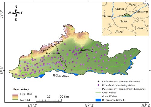
During July 17-21, 2021, the study area experienced a historically rare extreme rainfall event (‘7.20 Henan rainstorm’), with its heavy rainfall center in Jiaozuo and Xinxiang. The maximum daily precipitation was 505.6 mm (Wang et al. 2023). The torrential rain caused urban flooding and replenished groundwater, thus potentially alleviating the continuous decline in groundwater levels in the North China Plain. Taking the ‘7.20 Henan rainstorm’ as the background, this study focuses on the Downscaling Inversion of GRACE-Derived Groundwater Storage Changes in the research area to explore groundwater's response mechanism to the rainstorm. These results provide data and theoretical support for the rational development of groundwater resources in North China Plain.

2.2. Data

2.2.1. GRACE satellite data

The GRACE satellite data used in this study were the latest RL06 Mascon data product (Mascon) released by the Center for Space Research at the University of Texas, Austin (CSR). Mascon data provided information on the TWSA. The original spatial resolution of the data was 3° equal-area caps. However, in this data product, the spatial resolution was represented as 0.25° × 0.25°. The temporal resolution of this data product is monthly, and the data were acquired from October 2018 to August 2021 (https://www2.csr.utexas.edu/grace) (Save 2020; Save, Bettadpur, and Tapley 2016; Alghafli et al. 2023; Agarwal et al. 2023).

2.2.2. GLDAS dataset

The data set used in this study is provided by the Noah V2.1 (Noah) model in the Global Land Data Assimilation System (GLDAS), which was developed in collaboration with NASA and the National Oceanic and Atmospheric Administration (NOAA) (referred to as ‘Noah’ hereafter) (https://disc.gsfc.nasa.gov/) (McNally). The spatial and temporal resolutions of the Noah dataset were identical to those of the RL06 Mascon data. The GWSA can be obtained by combining the Noah data with the TWSA. The formula is as follows: (1) $GWSA=TWSA-SMA-SWA-\mathrm{SWEA}$(1) Among the variables used, Soil Moisture Anomalies (SMAs), Surface Water Anomalies (SWAs), and Snow Water Equivalent Anomalies (SWEAs) were derived from the ‘Noah model’ soil water (0-2 m depth), surface water, and snow water equivalent data, respectively. These values were obtained by subtracting 2004–01 to 2009–12 mean values from the corresponding variables to ensure consistency with the TWSA baseline (Lin, Biswas, and Bennett 2019; Sokneth et al. 2022). The impact of Biomass Anomalies (BMA) on GWSA is negligible and can be ignored (Liesch and Ohmer 2016).

2.2.3. National monitoring station groundwater level dataset

A dataset of continuous groundwater level observations with a 4-hour interval was obtained from national monitoring stations. There were 129 observational wells in the study area (Figure 1). The monthly average groundwater level data for each observation well ($GWL$) were compiled from October 2018 to August 2021. To ensure that the observation well dataset corresponded to the variations in the same baseline as the GRACE GWSA dataset obtained from Equation (1)(1) $GWSA=TWSA-SMA-SWA-\mathrm{SWEA}$(1) , considering the constraint of the ‘start and end times’, the observation well dataset, January to August 2021 was set as the target period for downscaling inversion. The mean groundwater level ($MGW{S}_{2018-2020}$) of each observation well from October 2018 to December 2020 and the mean GRACE GWSA data ($MGWS{A}_{2018-2020}$) within the same period were used as new baselines that needed to be subtracted from the $GWL$ and GRACE GWSA ($GWSA$) datasets, respectively. The formula is as below(Seyoum, Kwon, and Milewski 2019): (2) $GWS{A}_{2018-2020}^i=GWS{A}^i-MGWS{A}_{2018-2020}$(2) (3) $GWL{A}_{2018-2020}^i=GW{L}^i-MGW{L}_{2018-2020}$(3) Among them, i ($i\in [1,8]\cap Z^{+}$) represents the month, and $GWS{A}_{2018-2020}^i$ and $GWLA$ respectively refer to the modified baseline GRACE $GWSA$ dataset and the monthly average dataset of observed well data after establishing the baseline.

2.2.4. Other feature datasets

According to the commonly used groundwater influencing factor data (Agarwal et al. 2023; Liu et al. 2022; Miro and Famiglietti 2018; Sabzehee et al. 2023; Seyoum, Kwon, and Milewski 2019; Verma and Katpatal 2020) and some classical meteorological and hydrological features, the following data were obtained from Google Earth Engine, PIE-engine platform, and various official websites (Table 1), and feature datasets were processed.

Table 1. Summary of complete datasets information.

Datasets type	Datasets sources	Acquisition time of datasets	Characteristic informations
Static elements	SRTM (Shuttle Radar Topography Mission) (30m)	02/2000	Digital Elevation Model (DEM), Solp, Topographic Wetness Index (TWI), Drainage Density, Drainage Basin Density
	MODIS (Moderate-resolution Imaging Spectroradiometer) (250m)	01/01/2021-31/08/2021	NDVImax
	Landsat 8 OLI (Operational Land Imager) (30m)	01/01/2021-31/08/2021 (mean)	Modified Normalized Difference Water Index (MNDWI), MNDWI Distance, MNDWI Density
	GPWv411 (Gridded Population of the World Version 4.11) (30″)	2020	Population Density (P/Km²)
	CLCD (China Land Cover Dataset)(30m)	2020	Land Cover
	ISRIC (International Soil Reference and Information Center) (30″)	2004	Lithology
Dynamic elements	CHIRPS (Climate Hazards Group InfraRed Precipitation With Station) (0.05°)	01/01/2021-31/08/2021 (monthly mean)	Precipitation
	GCOM-C/SGLI L3 Land Surface Temperature (V2) (4638.3m)	01/01/2021-31/08/2021 (monthly mean)	Temperature (Daytime mean)
	FLDAS Noah Land Surface Model L4 Global Monthly (0.1°)	01/01/2021-31/08/2021 (monthly mean)	Soil Water (0-10cm), Evapotranspiration, Wind Speed
	Observation Well	01/10/2018-31/08/2021 (monthly mean)	GWLA
	GRACE (0.25°)	01/10/2018-31/08/2021 (monthly)	GWSA
	FLDAS Noah V2.1 (0.25°)	01/01/2004-31/12/2009 and 01/10/2018-31/08/2021 (monthly)	SMA, SWA, SWEA

MNDWI Density and Drainage Density are newly added features obtained by processing the raster data of the MNDWI greater than zero and drainage channel data using the Point Density tool in ArcGIS 10.6, with the population parameter values set as the MNDWI raster values and drainage channel flow, respectively. This feature represents the overall water density and drainage capacity in multiple directions at the grid points. The NDVImax was obtained using the maximum value composite method to reduce the effects of the atmosphere, such as clouds, fog, aerosols, cloud shadows, viewing angles, and sun altitude angles (Deng et al. 2022; Holben 1986).

An analysis of the groundwater influencing factors listed in Table 1 directly impacting the GWSA, positive and negative, was conducted. For example, precipitation, soil water, temperature, evapotranspiration, the MNDWI, and the MNDWI distance can directly affect groundwater recharge and depletion (Liu et al. 2022; Seyoum, Kwon, and Milewski 2019). The DEM, SOLP, TWI, drainage density, and drainage basin density significantly influence the flow direction and intensity of groundwater, making them the primary factors in the spatial variations of groundwater distribution (Liu et al. 2022; Miro and Famiglietti 2018).

Furthermore, the NDVI represents vegetation coverage. Studies have shown that vegetation cover in the watershed is greatly influenced by the GWSA (Liu et al. 2022; Sabzehee et al. 2023). By combining NDVI with land cover characteristics, the relationship between different vegetation types and groundwater storage can be revealed, especially in agricultural areas where the GWSA may be more susceptible to anthropogenic factors, such as agricultural irrigation (Agarwal et al. 2023; Sabzehee et al. 2023). Combining land cover with population density characteristics demonstrates the impact of urban water consumption on groundwater extraction (Agarwal et al. 2023; Sabzehee et al. 2023). Lithology and land cover illustrate the influence of subsurface conditions on the GWSA, as different lithologies and land cover types possess distinct hydraulic properties, such as transmissivity, specific yield, and specific capacity, affecting the groundwater storage capacity of different aquifer systems.

2.3. Methods

Based on data preprocessing, ensemble learning was introduced to invert the GWSA data. The steps included concatenating the unified baseline-adjusted GWSA and GWLA with the corresponding groundwater impact factor data from each monitoring well. Finally, the processed dataset was split into a base (90%) and holdout (10%) datasets. The holdout datasets were used to test the accuracy of the final output model. The base datasets are further divided during ML training, explained in detail in section 2.3.3. Then, using the GWLA values in the base datasets as the target values, multiple basic learners were trained, and all hyperparameters were optimized. According to the Root Mean Square Error (RMSE) mean of the fivefold cross-validation (CV), the top 2–5 basic learners were selected for ensemble learning and then optimized again for the hyperparameters. Finally, the ensemble models were validated using the holdout datasets. If the accuracy was low, the feature dataset and ensemble strategy were adjusted; however, if the accuracy met the expectations, the feature values of all grids (1 km × 1 km) were imported to obtain downscaled results. The data processing workflow is shown in Figure 2.

Figure 2. Data processing workflow.

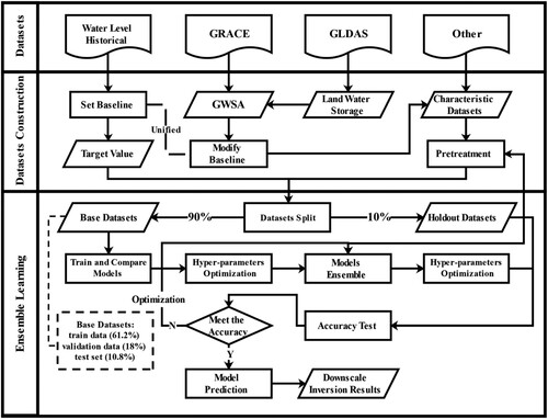
The model's accuracy was evaluated using a cross-validation method to prevent overfitting. Prior to ensemble learning, hyperparameter optimization was performed on all basic learners. After ensemble learning, the model underwent another round of hyperparameter optimization. This iterative process enhances the model's generalization ability and accuracy (Haq, Farooq Azam, and Vincent 2021).

2.3.1. Dataset optimization methods

Dynamic adjustments were made to the feature dataset by removing outliers and feature engineering. After each adjustment, all basic learners were trained 100 times, and the mean precision of the five-fold cross-validation was calculated. The precision of the dataset was compared after each adjustment, and the optimal feature dataset adjustment plan was obtained through the automatic traversal of all adjustable parameter combinations in Python. The following method was used to optimize the feature dataset for testing.

1. The removal of outliers can effectively reduce model bias. This study used Singular Value Decomposition (SVD) to identify outliers. This method removes outliers by selecting singular values, reconstructing the data, and dynamically setting a removal threshold to achieve optimal performance (PyCaret.org April 2020). SVD selects the top r singular values and reconstructs the data to remove outliers. The singular values are determined as follows (Sun, Yang, and Li 2022): (3) $X=US{V}^T$(3) where U and V are the left and right singular matrices consisting of left and right singular vectors, respectively, and S is a diagonal matrix that takes singular values as diagonal entries.

2. Binning converts continuous variables into categorical values using a predefined number of bins (PyCaret.org April 2020). This study used the K-means method to transform the numerical features into categorical features. This method iteratively solves the distance between each object and various seed cluster centers, assigns each object to the nearest cluster center, and recalculates the cluster centers based on the objects in the cluster. Iterative optimization causes the Sum of the Squared Errors (SSE) to reach a local minimum. In this study, the values in each bin had the same nearest center as in 1D K-means clustering.

2.3.2. Basic learner for Ensemble learning

Ensemble learning refers to aggregating a group of basic learners with varying performances to form a new model through specific ensemble methods to make predictions and compensate for errors produced by different basic learner results. The basic learners used in ensemble learning can be either homogeneous or heterogeneous. In this study, we compared and trained seven different basic learners: CatBoost (Gradient Boosting and Categorical Features), XGBoost (Extreme Gradient Boosting), LightGBM (Light Gradient Boosting Machine), GBDT (Gradient Boosting Decision Tree), Ada (AdaBoost), RF, and ET (Extra Trees).

1. GBDT

   The GBDT is an iterative decision-tree ensemble learning algorithm. The core idea is to iteratively construct a strong learner by serially combining multiple weak learners (Friedman 2002). At each iteration, a learner is built to reduce the loss along the steepest gradient direction to compensate for the deficiencies in the existing model. The final prediction results are obtained using weighted fusion (Johnson and Zhang 2013). When processing categorical features, the average value of the corresponding label ‘is used to replace the categorical feature and as the criterion for decision tree node splitting. Assuming that we are given a dataset $D=\{(X_i,Y_i){\}}_{i=1,2,\dots ,n}where{Y}_i\in Rand{X}_i=(x_{i,1},\dots ,x_{i,m})$ represents a vector of m features and label value. Categorical features $x_{i,k}$ are then replaced with their corresponding labels’ average values (Hancock and Khoshgoftaar 2020):

   (4) $x_{i,k}={\displaystyle \frac{{\sum }_{j=1}^n[x_{j,k}=x_{i,k}]Y_j}{{\sum }_{j=1}^n[x_{j,k}=x_{i,k}]}}$(4)

Among them, $[\cdot ]$ is the Iverson brackets, if $x_{j,k}$  = $x_{i,k}$, $[x_{j,k}=x_{i,k}]$equals 1 and 0 otherwise.

(2)

CatBoost CatBoost is a GBDT framework with fewer parameters, high accuracy, and support for categorical variables. It is implemented using symmetric decision trees as basic learners, consisting of Categorical and Boosting. The main innovation of CatBoost is its solution to the problems of gradient bias and prediction shifts (Hancock and Khoshgoftaar 2020; Prokhorenkova et al. 2018). In addition, the basic classifier in CatBoost is a balanced symmetric tree that can reduce the occurrence of overfitting, thereby improving the accuracy and generalization ability of the algorithm (Prokhorenkova et al. 2018). Unlike GBDT, CatBoost handles categorical features by adding an initial value to reduce noise, allowing the entire dataset to be used for training. Before the permutation, the average label value with the same category is calculated, and $x_{i,k}$ is replaced by it (Hancock and Khoshgoftaar 2020; Li et al. 2021): (5) $x_{{\sigma }_p,k}={\displaystyle \frac{{\sum }_{j=1}^{p-1}[x_{{\sigma }_{j,k}}=x_{{\sigma }_{p,k}}]Y_{{\sigma }_j}+a\cdot p}{{\sum }_{j=1}^{p-1}[x_{{\sigma }_{j,k}}=x_{{\sigma }_{p,k}}]Y_{{\sigma }_j}+a}}$(5) where $P$ represents a prior value, and a is its weight of the prior value ($a$,$p$ > 0).

(3)

XGBoost XGBoost is a large-scale, scalable ML system proposed by Tianqi Chen from the University of Washington, USA. This algorithm also optimizes the GBDT algorithm framework (Chen and Guestrin 2016; Kang et al. 2022). The advantage of XGBoost is that it performs a second-order Taylor expansion on the loss function, which increases accuracy, and a regularization term is added to the objective function to prevent overfitting. The objective function was as follows (Chen and Guestrin 2016; Liang et al. 2021): (6) $\mathrm{\Psi }(y,f(X))=\sum _{i=1}^N\mathrm{\Psi }(y_i,f(X_i))+\sum _{m=0}^T\left(\gamma L_m+{\displaystyle \frac{1}{2}\lambda {\omega }_m^2}\right)$(6)

Among them, $\mathrm{\Psi }$ represents the objective function, $N$ represents the number of features, $y_i$ represents the input value of the data, and $f(X_i)$ stands for prediction value, $L_m$ represents the number of leaf nodes and ${\omega }_m$ represents the influence of the $m$th leaf node on the model, $\gamma$ and $\lambda$ is regularization coefficients controlling the complexity of the model and the output of the objective function.

(4)

LightGBM LightGBM is an ML system that optimizes the gradient boosting decision tree (GBDT) algorithm by adding gradient-based one-sided sampling (GOSS) and Exclusive Feature Bundling (EFB) (Zhang, Lei, and Liu 2021). LightGBM uses a histogram algorithm to convert samples into intergroup complexity histograms and employs a unilateral gradient algorithm to filter out samples with small gradients during training, thereby reducing the computational complexity. LightGBM utilizes optimized features and data parallelism methods to optimize memory usage (Ke et al. 2017; Zhang, Lei, and Liu 2021). The GOSS algorithm retains all data instances with large gradients while randomly sampling data instances with small gradients and introducing a fixed multiplier to calculate the information gain in these instances to reduce the impact of the algorithm ‘on the data distribution (Gupta and Kumar 2023). This algorithm enables LightGBM to sample data based on each instance’, resulting in accurate estimates of information gain using smaller data sizes than GBDT. The EFB algorithm bundles many mutually exclusive features onto low-dimensional dense features, effectively avoiding unnecessary zero-feature value calculations without significantly affecting the split-point accuracy (Friedman 2001; Ke et al. 2017; Zhang, Lei, and Liu 2021).

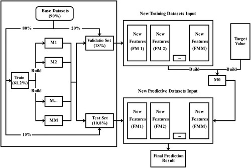
2.3.3. Blending ensemble method

Ensemble methods primarily include Blending and Stacker ensemble strategies, among which the blending ensemble algorithm is a model fusion method, as shown in Figure 3 (Li and Pan 2022).

1. The Blending ensemble method initially splits the base dataset into 80% base training data and 20% validation data. The base training data was further divided into 85% training data and 15% test sets. Therefore, the final base datasets were segmented into training, validation, and test sets, accounting for 61.2%, 18%, and 10.8% of the entire dataset (including holdout datasets), respectively.

2. In the first layer, M basic learner models were fitted to the training data, and predictions were made using the validation data and test set. These predictions create new features that serve as a training set for the second layer.

3. Metamodel M0 was trained using the new training data and target labels.

4. The test data were predicted using T-basic models, and the results were treated as new test data.

5. Meta-model M0 was used to predict the accuracy of the T-basic models on the new test data (Li and Pan 2022).

   In general, fusion methods include linear combinations and the use of basic learners for combinations. Using a complex fusion method in the second layer can easily result in overfitting in the blending ensemble method. Therefore, only a linear combination scheme is considered. This scheme uses a weighted average to assign each model M a different weight for better results. The formula used is as follows:

   (7) $G(x)=\sum _{t=1}^T{\alpha }_t\cdot M_t(x)with{\alpha }_i\ge 0$(7)

The value of ${\alpha }_t$ is determined using mean squared error: (8) $\underset{{\alpha }_i\ge 0}{min}{\displaystyle \frac{1}{n}\sum _{n=1}^N{\left[y_n-\sum _{t=1}^T{\alpha }_t{M}_t(x_n)\right]}^2}$(8) The model obtained using the blending ensemble method underwent hyperparameter optimization, and the model with the highest accuracy was selected for the output. Through continuous adjustments, once the accuracy of the model was satisfied, the final training of the model was conducted on the complete base datasets. This step is typically performed to improve the generalization ability and stability of the model. Subsequently, to verify whether the model was overfitting, a final test was conducted using the holdout datasets. If the accuracy of the model does not decrease significantly, it can be considered as the final model for prediction.

Figure 3. Blending ensemble method.

2.3.4. Permutation importance

In this study the model's performance was evaluated using two evaluation metrics: RMSE and R-Square (R²). RMSE measures the prediction error in regression models, whereas R² measures the goodness of fit of the regression model. RMSE and R² focus on different aspects: RMSE measures the difference between predicted and actual values, whereas R² assesses the model's explanatory power and goodness of fit (Uddin et al. 2022). A smaller RMSE indicates smaller prediction errors and better model fit, whereas R² ranges from 0 to 1, with values closer to 1 indicating a better fit. The equations for calculating these two evaluation metrics are as follows: (9) $RMSE=\sqrt{{\displaystyle \frac{1}{n}\sum _{i=1}^n{(y_i-{\hat{y}}_i)}^2}}$(9) (10) $R2=1-{\displaystyle \frac{{\sum }_{i=1}^n{(y_i-{\hat{y}}_i)}^2}{{\sum }_{i=1}^n{(y_i-\overline{y})}^2}}$(10) where $y_i$ represents the true value of the ith observation, ${\hat{y}}_i$ is the value predicted by the model, $\overline{y}$ is the average value of the true values, and $n$ is the number of samples.

2.3.5. Permutation importance

The PI index directly measures the importance of features by observing the impact of random permutations of each predictive attribute on the model's prediction accuracy. The PI is easy to calculate, the evaluation of feature importance is accurate, and its interpretability is relatively good (Breiman 2001).

The calculation process of this method is as follows (Breiman 2001):

1. The baseline model was trained, and the R² score was recorded as the benchmark score S using the validation set.

2. Feature $F_j$ in the dataset is selected sequentially. After each selection, the attribute values of $F_j$ must be shuffled and rearranged as $F_{m,j}$ (where m represents a certain shuffle among the M shuffles).

3. Establish a predictive model using the modified dataset and calculate the R² score $S_{m,j}$ using the validation set.

4. Calculate the feature importance $P_{F_j}$. The formula is: (11) $P_{F_j}=S-{\displaystyle \frac{1}{M}\sum _m^M{s}_{m,j}}$(11)

2.3.6. Z-Score normalization

The Z-score measures the number of standard deviations an original score deviates from the mean, which determines the position of the data in the entire dataset. The standardized indicator has a mean of 0 and a variance of 1 and has a good standardization effect when the sample data are greater than 30. The Z-score can process data with different dimensions and further analyze the relationship between groundwater response factors and groundwater level fluctuations. The conversion formula is as follows (Wu et al. 2001): (12) $Z={\displaystyle \frac{X-\overline{X}}{\sigma }}$(12) Among them, $X$ represents the raw data of a particular feature, $\overline{X}$ represents the mean value of the feature dataset, and $\sigma$ represents the standard deviation of the feature dataset.

2.3.7. Pearson product-moment correlation coefficient

The Pearson Product-moment Correlation Coefficient (PPMCC) was used to perform a correlation analysis between the groundwater storage anomaly (GWSA) inversion results from January to August in the study area and precipitation to examine the response of the GWSA to changes in precipitation. The calculation formula of PPMCC is as follows (Puth, Neuhäuser, and Ruxton 2014): (13) $R_{xy}={\displaystyle \frac{{\sum }_{i=1}^n(x_i-\overline{x})(y_i-\overline{y})}{\sqrt{{\sum }_{i=1}^n{(x_i-\overline{x})}^2{\sum }_{i=1}^n{(y_i-\overline{y})}^2}}}$(13) Here, $\overline{x}$ and $\overline{y}$ represent the mean values of variables x and y, respectively, and $R_{xy}$ represents the correlation coefficient between x and y. $R_{xy}$ ranges from −1 to 1, indicating a positive correlation between x and y when $R_{xy}$ is in the range of [0, 1], a negative correlation between x and y when $R_{xy}$ is in the range of [−1, 0], and no correlation between the two variables when $R_{xy}$ is 0.

2.3.8. Experimental environment

The experimental environment was set up using a machine equipped with the following specifications and software components.

1. Central Processing Unit (CPU): Intel(R) Core(TM) i9-9900K CPU at 3.60GHz

2. Random Access Memory (RAM): 48.0 GB

3. Dedicated Graphics Card: NVIDIA GeForce RTX 2080

4. Solid State Drive (SSD): INTEL SSDPEKKW512G8

5. Operating System: Windows 10

6. Python Version: Python 3.7.15

7. ML Framework: scikit-learn 1.0.2, pycaret 3.0.0

8. Other Libraries and Dependencies: pandas 1.3.5, matplotlib 3.5.3, numpy 1.21.6

3. Results

First, the training datasets were optimized using feature engineering methods. The data were then split into the dry and wet season subsets, trained separately, optimized for hyperparameters, and ensembled. Finally, the optimal downscaling inversion method was selected by comparing the mean RMSE and R² values obtained from the five-fold cross-validation.

3.1. Optimization and analysis of datasets

Using Python, we automatically traversed all possible parameter combinations and performed feature binning on several numerical features while adjusting the SVD threshold. Ultimately, we obtained the optimal feature dataset optimization scheme. (1) The SVD threshold was set to 0.05, meaning 5% of the outliers were removed from the training data. (2) The MNDWI, MNDWI Distance, and MNDWI Density features were binned, indicating that the weight of these feature values on the predicted target varied in different bins.

The mean accuracies of the five-fold CV before and after optimization are listed in Table 2 using the above scheme.

Table 2. Inversion accuracy before and after optimization of feature datasets.

Model	Before Optimization		After Optimization
	RMSE	R2	RMSE	R2
CatBoost	1.3344	0.7606	1.2944	0.7756
GBR	1.6404	0.6321	1.3295	0.7645
XGBoost	1.5115	0.6956	1.3304	0.7616
LightGBM	1.4894	0.7027	1.3780	0.7446
RF	1.5669	0.6699	1.5997	0.6561
ET	1.6161	0.6461	1.6665	0.6240
Ada	1.9212	0.4979	1.8090	0.5610

Table 2 shows that after optimizing the dataset, multiple basic learners’ R² and RMSE accuracy have significantly improved. Among them, GBR, XGBoost, LightGBM, and Ada have the most significant improvement in accuracy, with RMSA reduced by 18.95%, 11.98%, 7.48%, and 5.84%, respectively, and R² increased by 20.95%, 9.49%, 5.96%, and 12.67%, respectively. For RF and ET, R² and accuracy were slightly reduced, with RMSA increasing by 2.09% and 3.12% and R² decreasing by 2.06% and 3.42%, respectively. Therefore, this paper will use the optimized dataset for subsequent experiments and output the final downscaling results.

3.2. Seasonal split test between dry and rainy seasons

The study area has four distinct seasons, with significant differences in climatic characteristics between the dry and rainy seasons (Shi et al. 2022; Xu et al. 2021; Zhao-Kun et al. 2020). Considering that the main influencing factors of the GWSA are different in different climatic periods, the optimized January–August dataset can be split and tested using February to August as the starting month of the rainy season. The two datasets obtained after each split were separately trained, and the R² averages of the two training results were calculated. The results are shown in Figure 4.

Figure 4. Mean accuracy of split data sets in dry and rainy seasons.

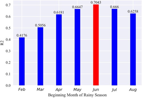
As shown in Figure 4, the R² mean value reached a maximum when June was set as the starting month of the rainy season, indicating the best data-splitting effect. Through an analysis of the seasonal variation characteristics of Henan Province over many years, Chang Jun et al. (Jun et al. 2011) concluded that the average summer start date in the province was May 31, consistent with the experimental results of this study. According to this splitting scheme, the January–May and June–August datasets can be obtained. Table 3 shows the five-fold CV accuracy mean values of this scheme.

Table 3. Accuracy obtained by training on split datasets.

Model	Jan-May		Jun-Aug
	RMSE	R2	RMSE	R2
CatBoost	0.9349	0.6328	1.9198	0.7573
XGBoost	0.9771	0.5992	1.8373	0.7758
GBR	0.9978	0.5798	1.9470	0.7516
LightGBM	1.0742	0.5176	1.9093	0.7593
RF	1.1577	0.4390	2.1302	0.7038
ET	1.2578	0.3419	2.1899	0.6861
Ada	1.2603	0.3244	2.1428	0.6958

As shown in Table 3, the R² values obtained from training with the June–August dataset are significantly higher than those obtained from training with the January–May dataset. The model trained with the June–August dataset had higher accuracy in the GWSA downscaling inversion.

3.3. Ensemble learning inversion analysis

The basic learner training results of the January–August, January May– and June–August datasets were ranked based on the RMSE value, and the top 2–5 basic learners with the lowest RMSE were selected for the ensemble using Blender and Stacker ensemble strategies. A linear combination was used for fusion for the Blender ensemble, whereas for the Stacker ensemble, both the linear combination and the best-performing basic learner were used. The five-fold CV mean results obtained after the ensemble are listed in Table 4.

Table 4. Inversion accuracy of models after ensemble learning.

Ensemble Method	Number of Ensembles	Jan-Aug		Jan-May		Jun-Aug
		RMSE(m)	R2	RMSE(m)	R2	RMSE(m)	R2
Blender (Linear Regression)	Top 2	1.2596	0.7887	0.9234	0.6423	1.7874	0.7891
	Top 3	1.2488	0.7921	0.9175	0.6472	1.7806	0.7905
	Top 4	1.2480	0.7924	0.9212	0.6444	1.7822	0.7904
	Top 5	1.2482	0.7922	0.9383	0.6316	1.7815	0.7903
Stacker (Linear Regression)	Top 2	1.3056	0.7788	0.9133	0.6489	2.0936	0.7129
	Top 3	1.3099	0.7775	0.9090	0.6512	2.1049	0.7093
	Top 4	1.3175	0.7740	0.9077	0.6497	2.0794	0.7166
	Top 5	1.3164	0.7744	0.9022	0.6553	2.1049	0.7098
Stacker (Optimal basic learner)	Top 2	1.3155	0.7751	0.9397	0.6337	1.8031	0.7831
	Top 3	1.3058	0.7785	0.9374	0.6279	1.8038	0.7845
	Top 4	1.3113	0.7757	0.9209	0.6451	1.8285	0.7807
	Top 5	1.2992	0.7794	0.9516	0.6219	1.8207	0.7821
Holdout (10%)		1.0547	0.7500	0.7202	0.3658	1.6256	0.8247

According to Table 4, for the January–August dataset, using the Blender ensemble strategy to linearly combine the top four basic learners with the lowest RMSE resulted in the best RMSE and R² values. Compared to the best individual basic learner, this ensemble scheme reduced the RMSE by 3.58% and increased R² by 2.17%. Similarly, for the January–May dataset, using the Blender ensemble strategy to linearly combine the top three basic learners with the highest RMSE accuracy yields the best RMSE and R² values. The RMSE was reduced by 1.86%, and R² increased by 2.28%. Using the Blender ensemble strategy to linearly combine the top three basic learners with the highest RMSE accuracy for the June- August dataset yielded the best RMSE and R² values. The RMSE was reduced by 3.09%, and R² increased by 1.89%. Through the application of ensemble learning, three optimal prediction models were obtained for the datasets mentioned above: ‘Model Jan-Aug,’ ‘Model Jan-May,’ and ‘Model Jun-Aug.’ Each of these models underwent a final round of training on their respective complete datasets, namely January–August, January May– and June–August, and were saved for future use (PyCaret.org April 2020). The parameter counts for the three models were 140, 153, and 116, respectively. The file sizes for these three models were 3.53MB, 4.16MB, and 1.74MB, respectively. The training times for these models were 305.9257, 695.0247, and 281.9329 s, respectively. The basic learners employed in these models include GBDT, CatBoost, XGBoost, and LightGBM.

As shown in Table 4, using the Blender ensemble strategy can improve model accuracy to a certain extent based on the basic learner. Both fusion schemes can improve the model accuracy to some extent for the Stacker ensemble strategy but still do not exceed the Blender ensemble strategy.

Ten percent of the reserved sets were randomly selected from each of the three datasets and reserved for the final accuracy test of the ensemble model without being involved in model training. The results show that the June–August model achieved the best accuracy, with an RMSE of 1.6256 and an R² of 0.8247, representing the overall best accuracy. The January–August model also achieved relatively high accuracy, with an RMSE of 1.0547 and an R² of 0.75. However, the January-May model obtained a lower accuracy result, with an R² value of only 0.3658. The R² value of the Jun-August model was 9.96% higher than that of the Jan-August model. Therefore, the June–August model can be used for the downscaling inversion of the GRACE GWSA in the study area from June to August, whereas the January–August model can be used for the downscaling inversion of the GRACE GWSA from January to May.

3.4. Analysis of downscaling inversion results

Using the January–August and June–August models, monthly GRACE GWSA data from January to August 2021 in the study area were downscaled to a resolution of 1 km. The monthly pixel mean of the GWSA (GWSAmean) and the Z-score standardized GRACE GWSA monthly pixel mean values were calculated for the cities of Jiaozuo and Xinxiang and are shown in Figure 5(a) and (b). Figure 5(c) and (d) show the GWSA of the observational wells and the corresponding downscaling inversion results for Jiaozuo and Xinxiang, respectively. The observation wells for each month in the figure were arranged in ascending order using DEM. The spatial distribution of the downscaled inversion results is shown in Figure 6.

Figure 5. Temporal statistics results of GWSA and its main influencing factors in Jiaozuo and Xinxiang cities.

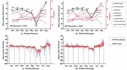
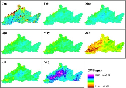
Figure 6. Monthly spatial distribution results of GWSA in Jiaozuo and Xinxiang cities.

3.4.1. Analysis of fitting performance of downscaling inversion results

As shown in Figure 5(a) and (b), in January, the GWSAwell, GRACE GWSAmean, and GWSAmean in Xinxiang City were all low, but the GWSAmean in Jiaozuo City was significantly lower than that in GWSAwell, and its trend was opposite to that of GWSAmean. Combined with the spatial distribution of low GWSA values in Figure 6 (January), the possible reasons for these results are: (1) The GRACE GWSA resolution is too low, and it is not sensitive to the distribution of local low GWSA values. (2) The distribution of observation wells in low-GWSA areas is sparse due to the geographical conditions in mountainous areas, making it difficult to use observation wells to monitor GWSA. Ensembling the GRACE GWSA with other influential datasets, such as GLDAS, using downscaling inversion by ensemble learning can effectively compensate for the deficiencies in monitoring GWSA through GRACE or observation well data alone. From February to August, the differences between GWSAmean and GWSAwell in the two cities were small, and the results were generally consistent. The overall trend of GWSAmean was consistent with that of GRACE GWSAmean, and both reached their first extreme points in March and April. In addition, both reached their minimum and maximum values simultaneously in May and August.

Graphs (c) and (d) show that the results of Models Jan-August and Jun-August for GWSA inversion in the study area were consistent with the GWSAwell results, with a good overall fit. From the variation in GWSA with DEM, it can be seen that the GWSA in Jiaozuo generally decreased with increasing DEM. In contrast, this phenomenon was less pronounced in Xinxiang, indicating that the spatial distribution of GWSA in Jiaozuo was significantly affected by topographic convergence.

3.4.2. Trend analysis of downscaling inversion results

After combining Figure 5 (a), (b), and Figure 6, it can be seen that the overall trends of GWSAmean in Jiaozuo City and Xinxiang City were the same. In January, the GWSAmean value in the study area was low, and the spatial distribution of GWSA was uneven, with low-value areas mainly distributed along the Taihang Mountains and the northern mining areas of the Macun District in Jiaozuo City. From February to March, GWSAmean increased significantly, reaching its peak in March, with Jiaozuo City and Xinxiang City having GWSAmean values of −0.1312 and 0.0337 m/km², respectively. The rising area was mainly the low-value anomaly area of the GWSA in January and the intersection area between Jiaozuo City and Xinxiang City. From April to May, the GWSAmean decreased significantly. The northern mountainous areas showed a significant decrease in GWSA in April, followed by a significant decrease in the GWSA southwest of Jiaozuo City in May. In June, GWSAmean dropped sharply to its lowest value, with Jiaozuo City and Xinxiang City having values of −6.0255 m/km² and −3.5850 m/km², respectively. The areas with severe GWSA depletion were mainly farmland and mountainous areas in southwest Jiaozuo City, centered on Fantian Town in Wen County, Jiegou Township in Wuzhi County, and Sanyang Township in Wuzhi County, with radii of approximately 25–30 km. The depleted area are distributed along both sides of the river. In July and August, GWSAmean increased sharply and reached its maximum value, with Jiaozuo City and Xinxiang City having values of 2.1016 and 1.4761 m/km², respectively. In August, the entire study area changed from loss to growth in the GWSA. In July, the growth of GWSA in Xiuwu County, Boai County, Qinyang City of Jiaozuo City, Fengquan District, Muye District, Huojia County, Xinxiang County, Yuanyang County, Yanjin County, Fengqiu County, and the Weihui City of Xinxiang City was the most significant, and the growth areas were primarily distributed on both sides of the Weihe, Dashaho, Jinti, Tianranwen Rock, and Communist Canals. In August, GWSA in Jincheng Township in Boai County, Muye District in Xinxiang City, Chenqiao Township, Caogang Township in Fengu County, and Nanpu Street in Changyuan City significantly increased. The growth areas were distributed around the Dashaho, Weihe, and Dashilao Rivers, indicating that the role of river water in replenishing groundwater levels was significant(Liu et al. 2022; Seyoum, Kwon, and Milewski 2019).

Both Figures 5 and 6 shows that the GWSA of Jiaozuo City and Xinxiang City exhibit a characteristic pattern of ‘slow rise-slow fall-rapid decline-rapid rise’ from January to August. Compared to Figure 5(a) and (b), the monthly GWSA mean variances of Jiaozuo City and Xinxiang City were 2.1293 and 1.3425, respectively. The fluctuation range of the GWSA in Jiaozuo was’ significantly greater than that in Xinxiang during the same period. However, the response of the GWSA to the July 20th Henan rainstorm was different between Jiaozuo City and Xinxiang City. In July and August, the groundwater level in Jiaozuo increased by 4.8746 and 3.2525 m/km², respectively, whereas that in Xinxiang increased by 2.9792 and 2.0819 m/km², respectively.

4. Discussion

The experimental results demonstrate that the spatiotemporal resolution achieved through downscaling inversion is superior than similar studies conducted in recent years (Agarwal et al. 2023; Miro and Famiglietti 2018; Sabzehee et al. 2023). Additionally, the Ensemble Learning method employed in this study achieved superior model accuracy compared to the basic learners used in similar studies conducted in recent years (Agarwal et al. 2023; Liu et al. 2022; Miro and Famiglietti 2018; Sabzehee et al. 2023; Seyoum, Kwon, and Milewski 2019; Verma and Katpatal 2020). The following discussion will be based on the results of downscaling inversion and will focus on ‘Permutation importance and correlation analysis’ and ‘Spatial analysis of GWSA anomalies.’

4.1. Permutation importance and correlation analysis

Figure 7 displays the PI results for Models Jan-August and Jun-August. Each feature was recalculated ten times after rearrangement, and the mean and variance of the resulting PI values were sorted. Here, we present the top 15 features with the highest mean PIs for both models (Breiman 2001). We standardized the Noah Snow water equivalent (SWE) (McNally) and dynamic elements with PI upper and lower quartiles both greater than 0.05 using the Z-Score and calculated their pixel means every month (as shown in Figure 5 (a) and (b)), to further analyze their correlation with GWSA.

Figure 7. PI Evaluation Results of Model Jan-Aug (a) and Model Jun-Aug (b). (a) Importance of permutations; (b) Importance of permutations.

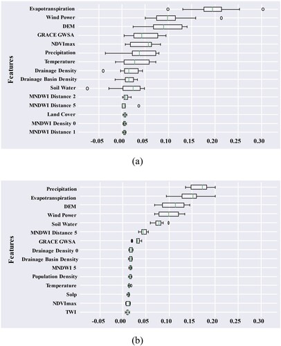
In January–August, the features with the highest PI values are evapotranspiration, wind speed, and DEM (Figure 7a), with the upper and lower quartiles of their PI values greater than 0.05. The highest features were GRACE GWSA, NDVImax, precipitation, and temperature, with PI values in the upper and lower quartiles close to 0.05. The PI values of these seven features were significantly higher than drainage density, drainage basin density, and soil water. Figure 5(a) and (b) show that evapotranspiration steadily increased from January to March, whereas precipitation remained low. Soil water sharply increased in March and reached its maximum, whereas wind speed rapidly decreased and reached its minimum in March. The SWE started to decrease rapidly after February. This indicates no melting of snow and ice in January, and groundwater has not been significantly replenished. In February and March, many sunny days with warm weather accelerated the melting of snow and ice and replenished groundwater. Moreover, in the Taihang Mountains region, groundwater is influenced by complex geological structures and terrain and flows toward urban areas. Therefore, the GESA increased most significantly in the Jiaozuo urban area. From April to May, precipitation increased slowly, but evapotranspiration increased more rapidly than precipitation. Soil water continued to decrease and reached its minimum in May when the SWE was zero. This indicates that snow and ice had almost completely melted in April and May, and there was little precipitation. With a continuous increase in evapotranspiration, the groundwater table drops rapidly, and the groundwater does not receive sufficient replenishment, leading to a sustained decrease.

In Figure 7(b), the features with the highest PI scores in the June–August model are precipitation, evapotranspiration, DEM, wind speed, and soil water. The PI scores of the upper and lower quartiles were all above 0.05, followed by the MNDWI distance fifth-bin feature and GRACE GWSA, with the PI scores of the upper and lower quartiles close to 0.05. The PI scores of these seven features were significantly higher than those of other features, whereas those of the remaining features PI scores are low and similar. Figure 5(a) and (b) show that precipitation slowly increased in May, evapotranspiration and soil water significantly increased, and wind speed sharply decreased, indicating more sunny days, and increased evapotranspiration, whereas precipitation does not increase significantly. Groundwater was not replenished by rainwater for a long time, leading to a decline in the GWSA. At the same time, groundwater in mountainous areas continuously flows to urban areas (Miro and Famiglietti 2018; Liu et al. 2022), resulting in severe groundwater depletion in mountainous areas. On the other hand, the increase in soil water content may be due to increased agricultural irrigation demand caused by less rainy weather, which also increases groundwater consumption. In July, the precipitation, evapotranspiration, and soil water content increased sharply. In August, precipitation decreased slightly but remained high, whereas evapotranspiration and soil water content remained high. Heavy rainfall from the July 20th Henan rainstorm replenished the groundwater. Although precipitation decreased slightly in August, the storms’ floods and surface water continue to replenish the groundwater for some time. The response of the GWSA to heavy rainfall has a certain lag, which is consistent with the conclusions of Luo et al. (Luo et al. 2020).

A comparison between Figure 7(a) and (b) reveals that during the dry season, the GWSA is mainly affected by evapotranspiration and SWE, whereas precipitation becomes the dominant factor during the rainy season. The PI value of the distance to water bodies also significantly increased, indicating that the rise in the water level of rivers and other water bodies during summer significantly impacted groundwater recharge. On the other hand, during the 7.20 Henan rainstorm period, the response of the GWSA to heavy rainfall was pronounced, and the impact of other factors on the GWSA became significantly smaller. Therefore, the downscaled inversion of the GRACE GWSA during June-August could lead to more seasonal characteristics and accurate results.

4.2. Spatial analysis of GWSA anomalies

Based on the interpretation of the PPMCC coefficient and land cover type distribution maps (Figure 8a and b), we conducted an analysis of the causes of GWSA anomalies in January, June, and August. The spatial distribution map of GWSA anomalies is displayed at the bottom of Figure 8.

Figure 8. Relationship between GWSA and precipitation and land cover in Jiaozuo and Xinxiang cities.

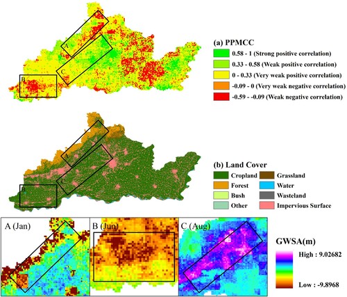
As shown in Figure 8(A), the GWSA in the region along the Taihang Mountains showed a strong positive correlation with precipitation. However, in the mountainous border area adjacent to the mountains, the GWSA showed a weak negative correlation with precipitation, indicating that the Taihang Mountains region is significantly influenced by precipitation, whereas the border area may be more affected by terrain convergence(Miro and Famiglietti 2018; Liu et al. 2022). In January, severe GWSA depletion was observed in the region along the Taihang Mountains in Jiaozuo City, mainly because of low precipitation and the fact that ice and snow had not yet melted, resulting in insufficient groundwater replenishment in the area. In addition, influenced by the terrain, the groundwater in the area continuously converges towards the mountainous border, accelerating groundwater depletion. Furthermore, the relevant literature indicates that land subsidence caused by coal mining in Jiaozuo City is mainly distributed in the coal-mining-intensive area of the Macun district (Jinjing et al.). In Figure 8(A), low GWSA values can be observed in the northern mining area of Macun District, including the Jiulishan and Fangzhuangxinjing mining areas, which may be due to long-term drainage and artificial groundwater mining in the mining area(Miro and Famiglietti 2018).

In the southwestern region of Jiaozuo City in June, the GWSA suffered serious deficits, as shown in Figure 8(B). This region's main land cover type is cropland, which showed a weak negative correlation with precipitation variation, indicating that precipitation change is not the main reason for the GWSA deficits in this area. Moreover, there are fewer mountains in the northern part of this area, indicating that the impact of terrain convergence on the GWSA is relatively small. Therefore, a possible cause of GWSA deficits in this area may be the increased demand for agricultural irrigation after the arrival of summer, which leads to increased groundwater losses. This is also supported by the increase in the soil moisture content in Jiaozuo City in June, as shown in Figure 5(a) and (b).

As shown in Figure 8(C), the area of sudden GWSA increase is mainly located at the edge of urban areas between Jiaozuo City and Xinxiang City and is distributed along rivers. The GWSA in this area was strongly positively correlated with precipitation change, and the main land cover type was cropland, whereas the main land cover types in the urban areas of Jiaozuo and Xinxiang were impervious surfaces. This indicates that during the Henan rainstorm on July 20, the impervious surface land cover type in the urban areas of Jiaozuo and Xinxiang affected the infiltration of precipitation, increased the drainage capacity of the urban areas, and most of the precipitation flowed into the surrounding rivers. The rise in the water level of these rivers will increase groundwater recharge around the rivers(Liu et al. 2022; Seyoum, Kwon, and Milewski 2019).

4.3. Study limitations and future directions

• In the application of ensemble learning, the dataset-splitting strategy is the optimal strategy obtained through multiple experiments and falls within the general range of empirical values(Haq, Jain, and Menon 2014; Verma and Katpatal 2020). When the sample size of the test set in the current optimal dataset-splitting strategy increases or decreases, the model's accuracy gradually decreases, leading to underfitting or overfitting. However, we still face challenges in the data collection process. However, if we apply the proposed method and train the model on a larger dataset, its quality may be further enhanced.

• Due to the challenges and limitations of data acquisition, many datasets that could potentially enhance the model's accuracy are difficult to obtain or validate. For example, (1) we did not estimate Sy. Estimating Sy can potentially improve the model's accuracy and stability. (2) For statistical reasons, it would be possible to achieve better downscaling inversion results if MGWSA and MGWL were calculated using longer time-series datasets or directly obtained GRACE Groundwater Storage (GWS) data.

5. Conclusions

Through the relevant experiments, this paper has drawn several conclusions:

1. By removing outliers and using feature engineering to bin MNDWI-related features, the precision of several basic learners in the five-fold cross-validation can be significantly improved. The RMSA can be reduced by up to 18.95%, and R² can be increased by up to 20.95%. By removing the outliers, the dataset can be optimized, leading to a significant reduction in noise impact, improved model fitting, and enhanced predictive capabilities.

2. The introduction of ensemble learning can effectively improve the accuracy of the downscaling inversion models. The five-fold cross-validation accuracy significantly improved when using the Blender ensemble strategy to combine several optimal basic learners trained on the June–August and January–August datasets. Furthermore, performing a Blender ensemble on the June–August dataset alone significantly improves the downscaling inversion accuracy during that period.

3. The monthly GWSA mean in the study area shows a characteristic trend of ‘slow increase-slow decrease-rapid decrease-rapid increase,’ with more significant fluctuations in the GWSA mean in Jiaozuo City. Generally, there was a slight variation in the GWSA mean from January to May. From July to August, the GWSA mean in Jiaozuo City and Xinxiang City continuously increased rapidly, reaching its peak in August for the entire study area. During June and August, the total groundwater storage in Jiaozuo City and Xinxiang City increased by 8.1271m/km² and 5.0611m/km², respectively, mainly due to the impact of the Henan rainstorm on July 20. Furthermore, heavy rainfall has a lagging effect on groundwater recharge.

4. Meteorological factors, such as precipitation and evapotranspiration, were the primary factors affecting the fluctuation of the GWSA mean in the study area. Terrain factors, such as DEM and drainage density, were the main influencing factors affecting the spatial distribution of groundwater in the study area. Changes in the spatial distribution of groundwater in the study area were greatly influenced by the terrain convergence of foothills and river valleys, and river leakage can significantly affect GWSA values. Additionally, human activities, such as coal mining and agricultural irrigation, significantly impact the GWSA. These findings are consistent with the conclusions of similar related studies (Agarwal et al. 2023; Liu et al. 2022; Miro and Famiglietti 2018; Sabzehee et al. 2023; Seyoum, Kwon, and Milewski 2019; Verma and Katpatal 2020).

Disclosure statement

No potential conflict of interest was reported by the author(s).

Data availability statement

The National monitoring station groundwater level dataset that support the findings of this study are available from Henan Provincial Bureau of Hydrology and Water Resources. Restrictions apply to the availability of these data, which were used under license for this study. Data are available from the Haiyang Yu([email protected]) with the permission of Henan Provincial Bureau of Hydrology and Water Resources. The authors confirm that the other datasets supporting the findings of this study are available within the article and its supplementary materials.

Additional information

Funding

This work was supported by National Natural Science Foundation of China: [grant no U1304402, 41977284]; Natural science and technology project of Department of Natural Resources of Henan Province: [grant no 2019-378-16].

References

- Agarwal, Vibhor, Orhan Akyilmaz, C. K. Shum, Wei Feng, Ting-Yi Yang, Ehsan Forootan, Tajdarul Hassan Syed, Umesh K Haritashya, and Metehan Uz. 2023. “Machine Learning Based Downscaling of GRACE-Estimated Groundwater in Central Valley, California.” Science of the Total Environment 865: 161138. doi:10.1016/j.scitotenv.2022.161138.
- Alghafli, Khaled, Xiaogang Shi, William Sloan, Mohammad Shamsudduha, Qiuhong Tang, Ahmed Sefelnasr, and Abdel Azim Ebraheem. 2023. “Groundwater Recharge Estimation Using in-Situ and GRACE Observations in the Eastern Region of the United Arab Emirates.” Science of the Total Environment, 161489. doi:10.1016/j.scitotenv.2023.161489.
- Atkinson, Peter M. 2013. “Downscaling in Remote Sensing.” International Journal of Applied Earth Observation and Geoinformation 22: 106–114. doi:10.1016/j.jag.2012.04.012.
- Baral, Prashant, and M. Anul Haq. 2020. “Spatial Prediction of Permafrost Occurrence in Sikkim Himalayas Using Logistic Regression, Random Forests, Support Vector Machines and Neural Networks.” Geomorphology 371: 107331. doi:10.1016/j.geomorph.2020.107331.
- Breiman, Leo. 2001. “Random Forests.” Machine Learning 45 (1): 5–32. doi:10.1023/A:1010933404324.
- Chen, Tianqi, and Carlos Guestrin. 2016. “Xgboost: A Scalable Tree Boosting System.” Paper Presented at the Proceedings of the 22nd acm Sigkdd International Conference on Knowledge Discovery and Data Mining.
- Deng, Guangyi, Jin Gao, Haibo Jiang, Dehao Li, Xue Wang, Yang Wen, Lianxi Sheng, and Chunguang He. 2022. “Response of Vegetation Variation to Climate Change and Human Activities in Semi-Arid Swamps.” Frontiers in Plant Science 13, doi:10.3389/fpls.2022.990592.
- Fatolazadeh, Farzam, Mehdi Eshagh, and Kalifa Goïta. 2020. “A New Approach for Generating Optimal GLDAS Hydrological Products and Uncertainties.” Science of the Total Environment 730: 138932. doi:10.1016/j.scitotenv.2020.138932.
- Friedman, Jerome H. 2001. “Greedy Function Approximation: A Gradient Boosting Machine.” Annals of Statistics, 1189–1232. doi:10.2307/2699986.
- Friedman, Jerome H. 2002. “Stochastic Gradient Boosting.” Computational Statistics & Data Analysis 38 (4): 367–378. doi:10.1016/S0167-9473(01)00065-2.
- Gao, Fei, Huixiao Wang, and Changming Liu. 2020. “Long-term Assessment of Groundwater Resources Carrying Capacity Using GRACE Data and Budyko Model.” Journal of Hydrology 588: 125042. doi:10.1016/j.jhydrol.2020.125042.
- Gong, Huili, Yun Pan, Longqun Zheng, Xiaojuan Li, Lin Zhu, Chong Zhang, Zhiyong Huang, Zhiping Li, Haigang Wang, and Chaofan Zhou. 2018. “Long-term Groundwater Storage Changes and Land Subsidence Development in the North China Plain (1971–2015).” Hydrogeology Journal 26 (5): 1417–1427. doi:10.1007/s10040-018-1768-4.
- Gosselin, David C, Venkataramana Sridhar, F Edwin Harvey, and James W Goeke. 2006. “Hydrological effects and groundwater fluctuations in interdunal environments in the Nebraska Sandhills.” Great Plains Research, 17–28.
- Gupta, Vaishali, and Ela Kumar. 2023. “H3O-LGBM: Hybrid Harris Hawk Optimization Based Light Gradient Boosting Machine Model for Real-Time Trading.” Artificial Intelligence Review:1-24, doi:10.1007/s10462-022-10323-0.
- Hancock, John T, and Taghi M Khoshgoftaar. 2020. “CatBoost for big data: an interdisciplinary review.” Journal of big Data 7 (1): 1–45. doi:10.1186/s40537-019-0278-0.
- Haq, Mohd Anul. 2021. “Intellligent Sustainable Agricultural Water Practice Using Multi Sensor Spatiotemporal Evolution.” Environmental Technology, 1–14. doi:10.1080/09593330.2021.2005151.
- Haq, Mohd Anul. 2022a. “CDLSTM: A Novel Model for Climate Change Forecasting.” Computers, Materials & Continua 71 (2): 2363–2381. doi:10.32604/cmc.2022.023059.
- Haq, Mohd Anul. 2022b. “CNN Based Automated Weed Detection System Using UAV Imagery.” Computer Systems Science and Engineering 42 (2): 837–849. doi:10.32604/csse.2022.023016.
- Haq, Mohd Anul. 2022c. “Planetscope Nanosatellites Image Classification Using Machine Learning.” Computer Systems Science and Engineering 42 (3): 1031–1046. doi:10.32604/csse.2022.023221.
- Haq, Mohd Anul. 2022d. “SMOTEDNN: A Novel Model for air Pollution Forecasting and AQI Classification.” Computers, Materials & Continua 71 (1), doi:10.32604/cmc.2022.021968.
- Haq, Mohd Anul, Prashant Baral, Shivaprakash Yaragal, and Biswajeet Pradhan. 2021. “Bulk Processing of Multi-Temporal Modis Data, Statistical Analyses and Machine Learning Algorithms to Understand Climate Variables in the Indian Himalayan Region.” Sensors 21 (21): 7416. doi:10.3390/s21217416.
- Haq, Mohd Anul, Mohd Farooq Azam, and Christian Vincent. 2021. “Efficiency of Artificial Neural Networks for Glacier ice-Thickness Estimation: A Case Study in Western Himalaya, India.” Journal of Glaciology 67 (264): 671–684. doi:10.1017/jog.2021.19.
- Haq, Mohd Anul, Abhijit Ghosh, Gazi Rahaman, and Prashant Baral. 2019. “Artificial Neural Network-Based Modeling of Snow Properties Using Field Data and Hyperspectral Imagery.” Natural Resource Modeling 32 (4): e12229. doi:10.1111/nrm.12229.
- Haq, Mohd Anul, Kamal Jain, and K. P. R. Menon. 2014. “Modelling of Gangotri Glacier Thickness and Volume Using an Artificial Neural Network.” International Journal of Remote Sensing 35 (16): 6035–6042. doi:10.1080/01431161.2014.943322.
- Haq, Mohd Anul, Abdul Khadar Jilani, and P. Prabu. 2021. “Deep Learning Based Modeling of Groundwater Storage Change.” Computers, Materials & Continua 70: 4599–4617. doi:10.32604/cmc.2022.020495.
- Haq, Mohd Anul, and Mohd Yawar Ali Khan. 2022. “Crop Water Requirements with Changing Climate in an Arid Region of Saudi Arabia.” Sustainability 14 (20): 13554. doi:10.3390/su142013554.
- Haq, Mohd Anul, Gazi Rahaman, Prashant Baral, and Abhijit Ghosh. 2021. “Deep Learning Based Supervised Image Classification Using UAV Images for Forest Areas Classification.” Journal of the Indian Society of Remote Sensing 49: 601–606. doi:10.1007/s12524-020-01231-3.
- Holben, Brent N. 1986. “Characteristics of Maximum-Value Composite Images from Temporal AVHRR Data.” International Journal of Remote Sensing 7 (11): 1417–1434. doi:10.1080/01431168608948945.
- Hsu, Ya-Ju, Yuning Fu, Roland Bürgmann, Shao-Yiu Hsu, Chin-Cheng Lin, Chi-Hsien Tang, and Yih-Min Wu. 2020. “Assessing Seasonal and Interannual Water Storage Variations in Taiwan Using Geodetic and Hydrological Data.” Earth and Planetary Science Letters 550: 116532. doi:10.1016/j.epsl.2020.116532.
- Jinjing, Lan, Qv Yiqiong, Du Weibing, and Gao Xin. 2022. “Surface Deformation and Analysis of Subsidence Characteristics in Typical Mining Cities by Remote Sensing.” Bulletin of Surveying and Mapping (06): 98–103. doi:10.13474/j.cnki.11-2246.2022.0179.
- Johnson, Rie, and Tong Zhang. 2013. “Learning Nonlinear Functions Using Regularized Greedy Forest.” IEEE Transactions on Pattern Analysis and Machine Intelligence 36 (5): 942–954. doi:10.1109/TPAMI.2013.159.
- Jun, Chang, Pan Pan, Wang Jijun, and Wu Yuanchao. 2011. “Analysis on Seasonal Variation Characteristics of Henan Province from 1957 to 2009.” Journal of Anhui Agricultural Sciences 39 (22): 13610–3. doi:10.13989/j.cnki.0517-6611.2011.22.015.
- Kang, Junfeng, Xingyu Guo, Lei Fang, Xiangrong Wang, and Zhengqiu Fan. 2022. “Integration of Internet Search Data to Predict Tourism Trends Using Spatial-Temporal XGBoost Composite Model.” International Journal of Geographical Information Science 36 (2): 236–252. doi:10.1080/13658816.2021.1934476.
- Ke, Guolin, Qi Meng, Thomas Finley, Taifeng Wang, Wei Chen, Weidong Ma, Qiwei Ye, and Tie-Yan Liu. 2017. “LightGBM: A Highly Efficient Gradient Boosting Decision Tree.” Paper Presented at the Proceedings of the 31st International Conference on Neural Information Processing Systems.
- Khorrami, Behnam, Shahram Gorjifard, Shoaib Ali, and Bakhtiar Feizizadeh. 2023. “Local-Scale Monitoring of Evapotranspiration Based on Downscaled GRACE Observations and Remotely Sensed Data: An Application of Terrestrial Water Balance Approach.” Earth Science Informatics, 1–17. doi:10.1007/s12145-023-00964-2.
- Li, Yang, and Yi Pan. 2022. “A Novel Ensemble Deep Learning Model for Stock Prediction Based on Stock Prices and News.” International Journal of Data Science Analytics, 1–11. doi:10.1007/s41060-021-00279-9.
- Li, Sijia, Kaishan Song, Shuai Wang, Ge Liu, Zhidan Wen, Yingxin Shang, Lili Lyu, Fangfang Chen, Shiqi Xu, and Hui Tao. 2021. “Quantification of Chlorophyll-a in Typical Lakes Across China Using Sentinel-2 MSI Imagery with Machine Learning Algorithm.” Science of the Total Environment 778: 146271. doi:10.1016/j.scitotenv.2021.146271.
- Liang, Heng, Kun Jiang, Tong-An Yan, and Guang-Hui Chen. 2021. “XGBoost: An Optimal Machine Learning Model with Just Structural Features to Discover MOF Adsorbents of Xe/Kr.” ACS Omega 6 (13): 9066–9076. doi:10.1021/acsomega.1c00100.
- Liang, Hao, Wei Qin, Kelin Hu, Hongbing Tao, and Baoguo Li. 2019. “Modelling Groundwater Level Dynamics Under Different Cropping Systems and Developing Groundwater Neutral Systems in the North China Plain.” Agricultural Water Management 213: 732–741. doi:10.1016/j.agwat.2018.11.022.
- Liesch, Tanja, and Marc Ohmer. 2016. “Comparison of GRACE Data and Groundwater Levels for the Assessment of Groundwater Depletion in Jordan.” Hydrogeology Journal 24: 1547–1563. doi:10.1007/s10040-016-1416-9.
- Lin, Mi, Asim Biswas, and Elena M Bennett. 2019. “Spatio-temporal Dynamics of Groundwater Storage Changes in the Yellow River Basin.” Journal of Environmental Management 235: 84–95. doi:10.1016/j.jenvman.2019.01.016.
- Liu, Qi, Dongwei Gui, Lei Zhang, Jie Niu, Heng Dai, Guanghui Wei, and Bill X Hu. 2022. “Simulation of Regional Groundwater Levels in Arid Regions Using Interpretable Machine Learning Models.” Science of the Total Environment 831: 154902. doi:10.1016/j.scitotenv.2022.154902.
- Luo, Zhanbin, Chenxu Yong, Jun Fan, Sheng Wang, and Mu Jin. 2020. “Precipitation Recharges the Shallow Groundwater of Check Dams in the Loessial Hilly and Gully Region of China.” Science of the Total Environment 742: 140625. doi:10.1016/j.scitotenv.2020.140625.
- McNally, A. “FLDAS Noah Land Surface Model L4 Global Monthly 0.1× 0.1 Degree (MERRA-2 and CHIRPS), Greenbelt, MD, USA, Goddard Earth Sciences Data and Information Services Center. 2018”.
- Miro, Michelle E, and James S Famiglietti. 2018. “Downscaling GRACE Remote Sensing Datasets to High-Resolution Groundwater Storage Change Maps of California's Central Valley.” Remote Sensing 10 (1): 143. doi:10.3390/rs10010143.
- Mollard, J. D. 1976. “Integration of Remote Sensing Techniques Applied to Groundwater Investigations.” Paper Presented at the Remote Sensing of Soil Moisture and Groundwater; Workshop Proceedings.
- Prokhorenkova, Liudmila, Gleb Gusev, Aleksandr Vorobev, Anna Veronika Dorogush, and Andrey Gulin. 2018. “CatBoost: Unbiased Boosting with Categorical Features.” Advances in Neural Information Processing Systems 31, doi:10.48550/arXiv.1706.09516.
- Puth, Marie-Therese, Markus Neuhäuser, and Graeme D. Ruxton. 2014. “Effective use of Pearson's Product–Moment Correlation Coefficient.” Animal Behaviour 93: 183–189. doi:10.1016/j.anbehav.2014.05.003.
- PyCaret.org. “PyCaret.” https://pycaret.org/.
- Rodell, Matthew, Isabella Velicogna, and James S Famiglietti. 2009. “Satellite-based Estimates of Groundwater Depletion in India.” Nature 460 (7258): 999–1002. doi:10.1038/nature08238.
- Sabzehee, F., A. R. Amiri-Simkooei, S. Iran-Pour, B. D. Vishwakarma, and R. Kerachian. 2023. “Enhancing Spatial Resolution of GRACE-Derived Groundwater Storage Anomalies in Urmia Catchment Using Machine Learning Downscaling Methods.” Journal of Environmental Management 330: 117180. doi:10.1016/j.jenvman.2022.117180.
- Save, Himanshu. 2020. “Csr Grace and Grace-fo rl06 Mascon Solutions v02.” Mascon Solut 12: 24. doi:10.15781/cgq9-nh24.
- Save, Himanshu, Srinivas Bettadpur, and Byron D Tapley. 2016. “High-resolution CSR GRACE RL05 Mascons.” Journal of Geophysical Research: Solid Earth 121 (10): 7547–7569. doi:10.1002/2016JB013007.
- Seyoum, Wondwosen M, Dongjae Kwon, and Adam M Milewski. 2019. “Downscaling GRACE TWSA Data Into High-Resolution Groundwater Level Anomaly Using Machine Learning-Based Models in a Glacial Aquifer System.” Remote Sensing 11 (7): 824. doi:10.3390/rs11070824.
- Seyoum, Wondwosen M, and Adam M Milewski. 2017. “Improved Methods for Estimating Local Terrestrial Water Dynamics from GRACE in the Northern High Plains.” Advances in Water Resources 110: 279–290. doi:10.1016/j.advwatres.2017.10.021.
- Shi, Lei, Zhongzheng Liu, Liangyan Yang, and Wangtao Fan. 2022. “Domestic Water use and Water-Saving Countermeasures in the Process of Urbanization in 2021: Jiaozuo City Case Study.” Water Science and Technology 85 (9): 2710–2721. doi:10.2166/wst.2022.116.
- Sokneth, Lim, S. Mohanasundaram, Sangam Shrestha, Mukand S Babel, and Salvatore GP Virdis. 2022. “Evaluating Aquifer Stress and Resilience with GRACE Information at Different Spatial Scales in Cambodia.” Hydrogeology Journal, doi:10.1007/s10040-022-02570-w.
- Sridhar, V., W. T. A. Jaksa, Bin Fang, Venkat Lakshmi, Kenneth G Hubbard, and Xin Jin. 2013. “Evaluating bias-corrected AMSR-E soil moisture using in situ observations and model estimates.” Vadose Zone Journal 12 (3), doi:10.2136/vzj2013.05.0093.
- Sun, Zhenlong, Jing Yang, and Xiaoye Li. 2022. “Differentially Private Singular Value Decomposition for Training Support Vector Machines.” Computational Intelligence and Neuroscience 2022), doi:10.1155/2022/2935975.
- Uddin, Md Galal, Stephen Nash, Mir Talas Mahammad Diganta, Azizur Rahman, and Agnieszka I Olbert. 2022. “Robust Machine Learning Algorithms for Predicting Coastal Water Quality Index.” Journal of Environmental Management 321: 115923. doi:10.1016/j.jenvman.2022.115923.
- Verma, Kaushlendra, and Yashwant B Katpatal. 2020. “Groundwater Monitoring Using GRACE and GLDAS Data After Downscaling Within Basaltic Aquifer System.” Groundwater 58 (1): 143–151. doi:10.1111/gwat.12929.
- Wahr, J. 2007. “Time-variable gravity from satellites.” Treatise on Geophysics 3: 213–237. doi:10.1016/B978-044452748-6/00176-0.
- Wang, Zhifeng, Bing Jiang, Xingtong Wang, Dongxu Wang, and Haihong Xue. 2023. “Psychological Challenges and Related Factors of Ordinary Residents after “7.20” Heavy Rainstorm Disaster in Zhengzhou: A Cross-Sectional Survey and Study.” BMC Psychology 11 (1): 1–13. doi:10.1186/s40359-022-01032-y.
- Whiting, J. M. 1976. “Airborne Thermal Infra red Sensing of Soil Moisture and Groundwater.” Paper Presented at the Remote Sensing of Soil Moisture and Groundwater; Workshop Proceedings.
- Wu, Hong, Michael J. Hayes, Albert Weiss, and Qi Hu. 2001. “An Evaluation of the Standardized Precipitation Index, the China-Z Index and the Statistical Z-Score.” International Journal of Climatology 21 (6): 745–758. doi:10.1002/joc.658.
- Xu, Wei, Fen Xu, Yunzhe Liu, and Dan Zhang. 2021. “Assessment of Rural Ecological Environment Development in China's Moderately Developed Areas: A Case Study of Xinxiang, Henan Province.” Environmental Monitoring and Assessment 193: 1–25. doi:10.1007/s10661-020-08746-9.
- Zhang, Chong, Qingyun Duan, Pat J-F Yeh, Yun Pan, Huili Gong, Wei Gong, Zhenhua Di, Xiaohui Lei, Weihong Liao, and Zhiyong Huang. 2020. “The Effectiveness of the South-to-North Water Diversion Middle Route Project on Water Delivery and Groundwater Recovery in North China Plain.” Water Resources Research 56 (10): e2019WR026759. doi:10.1029/2019WR026759.
- Zhang, Cheng, Xiujuan Lei, and Lian Liu. 2021. “Predicting Metabolite–Disease Associations Based on LightGBM Model.” Frontiers in Genetics 12: 660275. doi:10.3389/fgene.2021.660275.
- Zhang, Gangqiang, Wei Zheng, Wenjie Yin, and Weiwei Lei. 2020. “Improving the Resolution and Accuracy of Groundwater Level Anomalies Using the Machine Learning-Based Fusion Model in the North China Plain.” Sensors 21 (1): 46. doi:10.3390/s21010046.
- Zhao-Kun, Xu, Wei Zheng, Wenjie Yin, and Weiwei Lei. 2020. “Analysis of Groundwater Dynamic Monitoring in Xinxiang City.” Heilongjiang Science and Technology of Water Conservancy 48 (06): 9–11 + 117. doi:10.14122/j.cnki.hskj.2020.06.004.