Assessing factors impacting inter-satellite variability of grassland curing estimates for fire monitoring in Victoria, Australia using remote sensing

ABSTRACT

Grassland fires in Victoria, Australia pose significant environmental issues. Monitoring these fires relies on the Grassland Curing Degree (GCD) indicator and the corresponding Grassland Curing Map (GCM) for spatial distribution. Inter-satellite variability (ISV) assesses the variations in Grassland Curing Maps (GCMs) produced from remote sensing data with varying spatial resolutions (SR). Higher SR data improves GCM accuracy but increases processing time. ISV helps identify priority areas that need higher SR imageries. This study analyzes sample sites in Victoria and finds correlations between ISV, seasonality, temperature, precipitation, and distance to residential areas. Results reveal lower ISV during summers and autumns compared to winters and springs. Temperature shows a strong negative linear relationship with ISV, indicating that higher temperatures result in lower ISV. Precipitation exhibits a weak positive correlation with ISV, suggesting heavier precipitation leads to increased ISV. Distance to grasslands negatively correlates with ISV, indicating that greater distances from residential lands result in lower ISV. Based on these findings, it is recommended to use higher SR satellite data for GCM creation during winters and springs when temperatures are low, precipitation is heavy, and areas are closer to residential lands. Implementation suggestions are provided for fire management based on these results.

KEYWORDS:

• Grassland fire
• remote sensing
• environmental monitoring
• decision support
• GIS
• earth observation

1. Introduction

Grassland fires cause serious environmental problems in Victoria, Australia (Emergency Management Australia, Australasian Fire Authorities Council, and Country Fire Authority 2000; Forest Management Victoria 2021; Gullan 2021). Grassland curing degree (GCD) is one of the most important fire monitoring indicators which can be geo-located and converted to grassland curing maps (GCM) (Li 2020). Accurate estimates of grassland curing are needed for fire managers to understand fire risk, prepare resources, and determine fire spread during a fire event, therefore, a GCM of designated observing area contributes considerably to effectiveness and efficiency in fire monitoring.

Research on grassland curing via remote sensing provides valuable insights into the environment and its interactions with human activities. It enables monitoring and assessment of grassland fire risks, aiding fire agencies in predicting, preparing for, and preventing the impact of such fires on the environment over time (Fontana 2014; Wang et al. 2022). Furthermore, research on grassland curing plays a crucial role in shaping strategies for fire management and prevention, including prescribed burning and implementing fire breaks. Remote sensing technology enables the comprehensive gathering of data related to environmental factors like vegetation cover, moisture levels, and temperature, which proves essential in identifying areas at high risk of fire occurrences. (Brigitte, Laura, and Jesús 2012; Sharma and Dhakal 2021). Understanding the timing and locations of potential grassland fires becomes more achievable through this information, contributing to better fire prevention and management practices.

Over the last 20 years, there has been tremendous improvements in the geospatial technologies in terms of spectral, spatial and temporal resolutions (Maestrini and Basso 2018). It has been widely used for atmospheric environment, water environment and ecological environment protection and monitoring (Zhao et al. 2017). In recent years, literature shows increasing popularity for combined usage of various satellite sensors, but most fire products were created from sensors that were designed for other purposes (Chuvieco et al. 2020). From the latest grassland literature, it has not only verified the usage of remote sensing satellite data for grassland observation and grassland fire monitoring, but also suggested the importance of using high SR satellite data to calculate GCD for distinct regions and during different seasons (Li 2020; 2021). It is found that different SR satellites lead to variations in GCD and that the larger the difference in SR, the greater the ISV is; ISV also varies with seasonality (Li 2021). These studies have laid the groundwork for extensive grassland observation and fire monitoring using satellite data with different spatial resolutions across various locations and timeframes. Building upon this foundation, this paper aims to delve deeper into the inter-satellite variability (ISV) between Grassland Curing Maps (GCM) generated at different spatial resolutions and its associated influencing factors, using more extensive and long-term datasets than previous research.

For the same area observation extent, the higher the SR of the satellite remote sensing data is, the larger the quantity of data there is, and the more localized the GCD calculations are, which leads to higher accuracy GCM. With the increase in the accuracy of GCM, the data quantity exponentially increases at the same time, and the processing time also increases significantly which leads to substantial increases in labor costs. Therefore, with the most efficient resource and time allocation as the goal, it is imperative to adopt a system for the most productive distribution of resources for GCM creations while maintaining high quality. Selecting the appropriate type of satellite remote sensing data for a particular observation area and appropriate times can greatly reduce the time and labor cost. In other words, it is important to determine when, where, and what SR satellite remote sensing data should be used.

In light of the above research aim, research objectives and questions are identified in this study: (1) to determine the ISV of grassland curing in Victoria using satellite remote sensing data from 2016 to 2020; (2) to assess the ISV from GCM created from sensors with different SRs (Sentinel 2, Landsat 8 and MODIS); (3) to explore ISV distribution patterns and factors that impact ISV and to develop a decision support system. To answer these research questions, this study begins with calculation and analysis of GCD and GCM. Followed by examining the differences and characteristics of GCD and GCM by calculating the ISV which displays the differences in GCD of GCM. Next, the correlations between ISV and impact factors including seasons, temperature, precipitation, and distance are analyzed. Lastly, specific and practical recommendations along with a straightforward decision-making model is created for grassland fire managers to establish effective and efficient fire monitoring and prevention system. The findings will help to determine the location, time or season, and climatic conditions where satellite remote sensing data of different SRs should be used when producing GCM at the maximum efficiency. It provides scientific basis for effective grassland fire monitoring and recommendations to fire authorities and decision-makers to help strategize and implement fire monitoring systems.

2. Data and methodology

2.1. Data

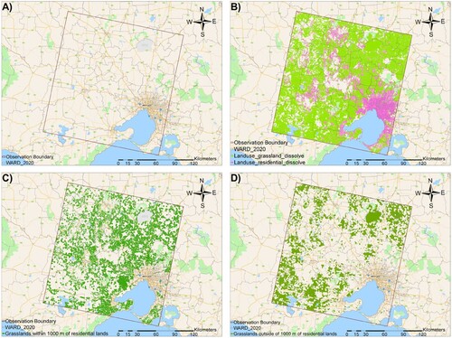
Five years of MODIS and Landsat 8 satellite data from 2016 to 2020 were used to calculate ISV and determine the relationship between ISV and seasonality; followed by analysis and discussion of ISV and its impact factors including distance to residential lands, temperature, and precipitation. The study area is outlined in Figure 1(A).

Figure 1. (A) Observation extent. (B) Grasslands and residential lands. (C) Grasslands within 1000 m of residential lands. (D) Grasslands outside of 1000 m of residential lands.

The data used in this study includes MODIS (500 m) and Landsat 8 (30 m) satellite data from the United States Geological Survey (USGS) database. There are 40 images used in total to produce 40 grassland curing maps and 20 ISV maps. One image from each season over five years from 2016 to 2020 is taken for each satellite. In this research, seasonality matches the geographical location of Australia: Summer months are December, January, and February; Autumn months are March, April, and May; Winter months are June, July, August; Spring months are September, October, and November. Image selection is based on cloud percentage and the time of the image. Images with the least cloud cover are prioritized; if there are multiple clear images, then the image closest to the middle of the season is prioritized. Sensors on board of the satellites have radiometric resolutions of 12 bits (European Space Agency 2021; National Aeronautics and Space Administration 2021a; 2021b) and measurements are converted to reflectance and stored as 16-bit integers for this study.

Terra MODIS MOD09A1 Version 6 products satellite data are used for this study. They have been corrected for atmospheric conditions such as gasses, aerosols, and Rayleigh scattering. There are seven 500 m reflectance bands covering wavelengths in the visible (VIS), NIR, SWIR, and mid-wave infrared (MWIR) and additionally two quality layers and four observation bands (Vermote 2015).

Landsat 8 data used for this study are scenes observed with a combination of OLI and TIRS downloaded from USGS though EarthExplorer. They are processed to the best available processing level of Level-1 precision and terrain corrected product (L1TP), meaning the data has been atmospherically corrected by the EROS ESPA on-demand interface. The Landsat 8 data used in this study contains 11 spectral bands in the visible, NIR and SWIR part of the spectrum (NASA 2021c).

The land use map is the newest available dataset from VLUIS for 2017 created by the Spatial Information Sciences Group of the Agriculture Victoria Research. This shapefile covers the entire landmass of Victoria and separately describes the land tenure, land use and land cover across the state at the cadastral parcel level (Department of Jobs, Precincts and Regions 2018). These data have an attribute table linking the land use information to the geographical locations on the map layer.

WARD_2020 is a base map outlining the local government regions for the state of Victoria. It is used in this study as a background to all other map layers to provide a visual support for the GCM to help readers understand where GCM are mapped. This shapefile is obtained from the VicMap Admin dataset series.

There are also base maps in ArcGIS Pro’s gallery. The one in use for this study is the ‘World Topographic Map’.

2.2. Curing calculation

2.2.1. Curing calculation model

This research adapts GCD calculation used by Li (2020). The author states that:

GCD is calculated using the equations from MapVictoria with appropriate adjustments to the results. Curing degree is calculated as:

1. $\mathrm{Curing}=(\mathrm{NDVI}\times -88.41)+(\mathrm{GVMI}\times -67.71)+113.80$ where

2. $\mathrm{NDVI}={\displaystyle \frac{\mathrm{NIR}-\mathrm{Red}}{\mathrm{NIR}+\mathrm{Red}}}$ and

3. $\mathrm{GVMI}={\displaystyle \frac{(\mathrm{NIR}+0.1)-(\mathrm{SWIR}+0.02)}{(\mathrm{NIR}+0.1)+(\mathrm{SWIR}+0.02)}}$ where

4. $\mathrm{SWIR}$’s bandwidth is in approximate range of 1628–1652 nm.

Curing, or GCD, indicates how much dry contents the grass has. 100% cured would mean the grass is completely dried and dead where 0% cured would mean the grass is fresh and all parts are alive and usually green (Li 2021).

Data are processed under the ArcGIS Pro environment with arcpy, spatial analyst, and image analyst packages using PyCharm.

2.2.2. Land use data correction and preparation

Figure 2(A) summarizes the process and usage of land use images for differentiating grasslands and residential lands. This is followed by further construction of 1000 m buffer area around residential lands for the examination of grasslands within and outside of 1000 m of residential lands.

Figure 2. (A) Land use data correction and preparation. (B) Landsat data processing. (C) MODIS data preparation and processing. (D) Comparable data preparation.

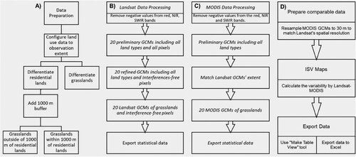
Land use image and data files are configured to match the observation extend of this research. Then image features are extracted to form coherent and homogenous residential lands map and grasslands map (Figure 1(B)). A 1000 m buffer was added to the perimeter of the boundary of residential lands that produced images for analysis of grasslands within and outside of 1000 m of residential lands (Figure 1(C,D)).

2.2.3. Landsat data processing

Figure 2(B) shows the flowchart of Landsat data processing. Because the Landsat data used for this study have been terrain corrected, there are some negative values in the raster bands. To prevent calculation error for indices required for GCD calculations, the first step is to nullify all the negative values from the red, NIR, and SWIR bands that are used for GCD calculation and GCM construction. This generated 20 preliminary GCM for all four seasons from 2016 to 2020.

To eliminate interference such as clouds, water, shadows, snow and ice from the preliminary GCM, only ‘clear’ pixels are extracted via the Pixel Quality Assessment (pixel_qa) band generated by the C version of the Function of Mask (CFMask) algorithm (US Geological Survey 2020). This refined the preliminary GCM by removing interferences.

The refined GCM then removes all other land types but areas with ‘grassland’ attributes from the land use image. By combining the refined GCM with the grassland land use image, all GCM have the same observation extent. This created 20 GCM for all four seasons from 2016 to 2020.

For further statistical analysis of the final 20 Landsat GCM, it is important to export all the numerical data. GCD were stored as floats, a floating-point number that has a decimal place. However, for more efficient and simpler data analysis, floats were converted into unsigned 16-bit short integers that are whole numbers and without fractional components. The impact of truncation is negligible because grassland curing estimates are commonly estimated to the nearest tenth, therefore, having integers between each 10% is a huge increase in precision. In this way, instead of numerous GCD values with frequency of one, there are only 101 possible values for GCD (0–100) with a higher frequency for each integer. All numerical data and GCM are exported and stored as Microsoft Excel spreadsheets.

2.2.4. MODIS data preparation and processing

Figure 2(C) shows MODIS data processing. The Terra MODIS MOD09A1 Version 6 product data downloaded from USGS have been corrected for atmospheric conditions, therefore there are also some reflectance values in the invalid range. Hence the negative values are nullified.

Similar to processing the Landsat data, preliminary GCM including all land types and all pixel qualities are made with the red, NIR and SWIR2 bands.

Since the boundary of clear Landsat scenes has already been produced, the MODIS scenes can use the same boundary file to match the observation extent of the Landsat GCM. This produced 20 MODIS GCM.

After converting float numbers to integers of the MODIS GCM, they are also exported to Microsoft Excel spreadsheets (Figure 2(D)).

2.3. ISV

2.3.1. Choosing ISV impact factors

There are three factors chosen in this study to analyze their relationships with ISV: distance to residential lands, temperature, and precipitation. Grassland fire monitoring is especially important for areas near residential areas because the potential damage, such as loss of homes and lives, could be much greater than areas with just grasslands. However, when grasslands are closer to residential lands, the boundaries of grass and infrastructure becomes more difficult to discern. Therefore, understanding the relationship between ISV and distance to residential lands is important in grassland fire monitoring.

Temperature is one of the chosen impact factors because grassland curing strongly correlates to temperature. The natural cycle of growth cycle dictates when to grow, wilt or become dormant; with this natural cycle, there are four seasons and each season have their representative temperatures—winter is the coolest, and summer is the hottest. Knowing the relationship between ISV and temperature can help understand what temperatures are easy or difficult for grassland curing estimations.

Another important factor that impacts ISV is precipitation. Precipitation has been adjusted to antecedent precipitation index (API) to account for effective previous rainfall. API, represents the accumulation of daily precipitation amounts through a weighted sum, reflecting the impact of accumulated precipitation (Li, Wei, and Li 2021; Xie and Yang 2013). There is a time lag of few weeks for precipitation to reflect in GCD estimations, but after the rainfalls, grass grow, and GCD lowers. However, the decrease in GCD could be due to multiple reasons such as new grass germination or re-greening of the yellow grass; this does not apply to all grass. Therefore, increasing the variation of GCD will increase ISV. Choosing precipitation as a factor is mainly to assess to what extent does precipitation affect ISV.

2.3.2. ISV maps

The GCM created by Landsat and MODIS were compared to create ISV maps. All 20 Landsat 8 GCM, one from each season and five years in total, are paired to MODIS GCM respectively. The absolute value of their spatial differences is ISV and associated with geographical locations to produce ISV maps. In this way, a total of 20 ISV maps are generated. Through paired GCM comparisons, the relationship between resolution difference and ISV can be captured quantitatively. Steps are shown in Figure 2(D).

With the purpose of contrasting the GCM produced from Landsat and MODIS, they must be comparable. The Landsat GCM have a SR of 30 m and the MODIS ones have a SR of 500 m. To match the higher SR of the Landsat GCM, MODIS GCM were resampled using ArcGIS Pro from 500 m to 30 m.

ISV is the difference between the GCD calculated using different satellite data. Here, the absolute values of Landsat minus MODIS GCD are the ISV and mapped as ISV maps.

Finally, ISV statistics were made into a table view and exported for further analysis.

2.3.3. Categorizing ISV

ISV are categorized into three groups: ‘0–4’, ‘5–20’, ‘20+’ based on the magnitude of the ISV. Group one ‘0–4’ is for small and negligible ISV. Group two ‘5–20’ indicates where there are significant GCD differences as observed by the two satellites. Group three ‘20+’ is for unusually large ISV and they comprise less than 10% of the entire dataset. When ISV is less than five, the difference in GCD is marginal and can be considered as no substantial difference in the satellite data used. Group two ‘5–20’ is the most important category as it indicates where significant GCD calculation difference exists due to the satellite data used. Because GCM commonly classify curing degrees into every 10 degrees, rounding errors will occur most frequently when there is a difference greater than five degrees. Therefore, ISV of 5–20 are considerable differences. Group four ‘20+’ contains barely any data, and are mostly due to residual clouds.

2.4. Correlation analysis

To establish the strength of the correlation between ISV and the various factors, correlation tests have been done. Since distance to residential lands has been set to 1000 m, the result can only compare outside of 1000 m versus within 1000 m of residential lands rather than how strongly distance to residential lands correlates to ISV. 0–4 ISV will always have near perfect positive correlation with 0–4 ISVi and 0–4 ISVo; and near perfect negative correlation with 5–20 ISV, 5–20 ISVi, and 5–20 ISVo. similarly, 5–20 ISV will have very highly positive correlation with 5–20 ISVi, and 5–20 ISVo; and very highly negative correlation with 0–4ISV, 0–4 ISVi and 0–4 ISVo.

The strength of the correlation between ISV to temperature and API can be calculated by pairing ISV to temperature and API respectively according to the date. When the magnitude or the absolute value of the correlation coefficient is between 0.9 and 1.0, it indicates variables are very highly correlated; if it is between 0.7 and 0.9, variables are considered highly correlated; if the magnitude of the correlation coefficient is between 0.5–0.7, variables are moderately correlated; 0.3–0.5 indicates variables have a low correlation; and if the absolute value of the correlation coefficient is less than 0.3, the variables have little to no linear relationship (Calkins 2005).

3. Results and analysis

In order to verify and extend on previous chapters’ results, this section analyzes the characteristics of ISV over five years to explore the relationship between ISV and seasonality. Data are collected from 2016 to 2020 to calculate ISV between the GCD estimated by Landsat 8 and MODIS. The summary statistics of ISV for each season are shown in Table 1.

Table 1. 2016–2020 ISV statistics. Summer: December–February; Autumn: March–June; Winter: July–September; Spring: October–November.

ISV	Season	Average (%)	Range (%)	Fluctuation (%)
0–4	Summer	43	39–46	7
	Autumn	37	29–49	20
	Winter	23	20–26	6
	Spring	25	21–30	8
5–20	Summer	45	43–48	5
	Autumn	49	40–57	18
	Winter	57	54–60	7
	Spring	59	53–61	8
20+	Summer	12	10–13	3
	Autumn	14	12–16	4
	Winter	20	17–25	8
	Spring	16	11–26	15

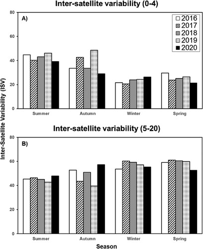
3.1. Seasonal and yearly ISV

From Table 1, the largest fluctuations are 20% and 18% which occurred during autumn for both low (0–4) and high (5–20) ISV. The other three seasons, summer, winter, and spring, have smaller fluctuation and their values are similar between 5% and 8% for both low (0–4) and high (5–20) ISV. This reveals that autumn is the season that affects ISV the most.

Figure 3 provides insights on the percentage of low and high ISV between 0–4 and 5–20 for different seasons and years. The average percentage of low ISV is the highest during summer at 43%, followed by autumn at 37%, and is drastically lower during winter and spring at 23% and 25%, respectively. This suggests that summer and autumn are the best seasons for accurately distinguishing grassland canopy density (GCD) through satellite observations due to lower ISV. On the other hand, the percentage of high ISV is the highest during spring and winter at 59% and 57%, respectively, and shows a noticeable decline in summer and autumn at 45% and 49%. These findings imply that GCD calculations during winter and spring have a higher chance of error due to a large percentage of high ISV.

Figure 3. Seasonal and yearly ISV. (A) ISV 0–4. (B) ISV 5–20.

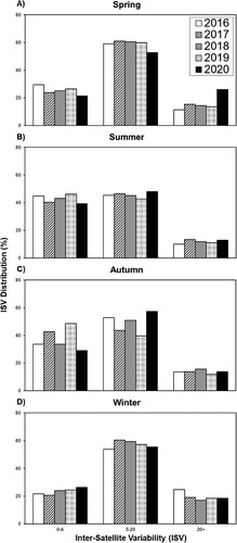
3.2. ISV distribution

ISV was analyzed in relation to the different seasons using remote sensing satellite data over a period of 5 years (Figure 4). The results showed that the average percentage of ISV between 0–4 was lower than that of 5–20 in spring, winter, and autumn. In spring, there were more ISV between 5–20, indicating a lower ability to detect grassland curing accurately in that season. Summer showed similar percentage distributions of low and high ISV, around 40–50%. In autumn, the average percentage of low ISV was slightly lower than that of high ISV, with a significant variation from year to year, likely due to temperature changes. In winter, the average percentage of low ISV was significantly lower than that of high ISV, indicating the lowest ability to detect grassland curing accurately among all seasons. These findings could provide decision-makers in fire monitoring with a scientific basis for using satellite data for grassland fire monitoring and help to improve the management and conservation of grassland ecosystems.

Figure 4. ISV distribution 2016–2020. (A) Spring. (B) Summer. (C) Autumn. (D) Winte.

3.3. Distance and ISV

In this section, ‘_i’ represents grassland within 1000 m of residential lands and ‘_o’ represents grassland outside of 1000 m of residential lands (Table 2).

Table 2. ISV statistics – within 1000 m of residential lands vs. outside of 1000 m of residential lands.

	ISV	Peak values	Trough values	Mean value	Mean value difference	Peak months	Trough months
All ISV	0–4	39–49	20–26	32	20	January–March	June–September
	5–20	53–61	39–48	53		June–September	January–March
ISV within 1000 m of residential lands (ISVi)	0–4i	37–43	20–26	31	23	January–March	June–September
	5–20i	54–61	43–49	54		June–September	January–March
ISV outside of 1000 m of residential lands (ISVo)	0–4o	42–56	20–27	35	16	January–March	June–September
	5–20o	52–61	34–46	51		June–September	January–March

Figure 5(A) compares all low ISV to all high ISV. It is as anticipated that both trends oscillate opposite to each other. The entire ISV distribution is divided into 0–4, 5–20 and 20+; 0–4 and 5–20 comprise almost up to 90% of the data. Therefore, the pattern of 0–4 is opposite to that of 5–20.

Figure 5. Time series of ISV 0–4 vs. 5–20 distribution. (A) All ISV. (B) ISV within 1000 m of grasslands. (C) ISV outside of 1000 m of grasslands.

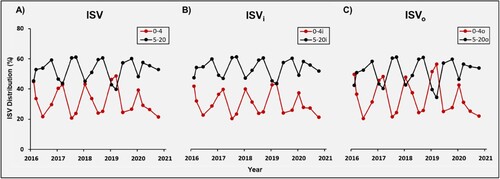
The two curves intersect or meet from January to March during late summer or early autumn months. This happens when both curves have steep slopes of increase or decrease around the same time. This shows that the greatest fluctuation in ISV occurs when season progresses from summer to autumn.

Figure 5(B) has a similar trend to that of Figure 5(A), but further apart. It indicates an increase in ISV that are between 5–20 and a decrease in ISV that are between 0–4. This is because the average of 5–20 is higher and the average of 0–4 is lower. The magnitude between low and high ISV is larger.

In Figure 5(B), ISV between 0–4_i have less percentage than Figure 5(A)’s 0–4, and 5–20_i has an increase when closer to residential lands. This means that less areas have low ISV, and more areas have large ISV. The closer it is to residential lands, the harder it is to distinguish GCD accurately, so the need for higher SR satellite increases.

Figure 5(C) has a trend similar to Figure 5(A), but the lines are closer together due to lower averages for 5–20 and higher averages for 0–4. This is because the average of 5–20 is lower and the average of 0–4 is higher. The magnitude between low and high ISV is smaller.

Figure 5(C) depicts the lands that are further away from residential area. Its 0–4 has more percentage than Figure 5(A) and 5–20 has less when further away from the residential lands. This means that more areas have low ISV, and less areas have large ISV. The further it is to residential lands, the easier it is to distinguish GCD accurately, so the need for higher SR satellite decreases.

In conclusion, distance has impact on ISV since satellite imagery data cannot separate the adjacent boundaries of residential lands and grassland precisely. The shorter the distance to residential areas, the higher the difficulty to distinguish GCD; therefore, the necessity for higher SR satellite is stronger.

3.4. ISV vs. Temperature and API

Temperature plays a crucial role in influencing ISV as shown in Figure 6(A). The pattern of daily temperature is similar to that of low ISV 0–4, with peak months of January to March and trough months of June to September. This indicates that temperature has a strong positive relationship to ISV in the classes 0–4, 0–4i, and 0–4o, regardless of the distance to residential lands. Moreover, the ability to detect accurate GCD becomes stronger in warmer months, resulting in lower ISV. The positive relationship between temperature and ISV is further supported by Figure 6(B,C), which compare temperature to ISV within and outside of 1000 m of residential lands.

Figure 6. Time series of ISV 0–4 vs. 5–20 distribution and temperature/API. (A) All ISV and temperature. (B) ISV within 1000 m of grasslands and temperature. (C) ISV outside of 1000 m of grasslands and temperature. (D) All ISV and API. (E) ISV within 1000 m of grasslands and API. (F) ISV outside of 1000 m of grasslands and API.

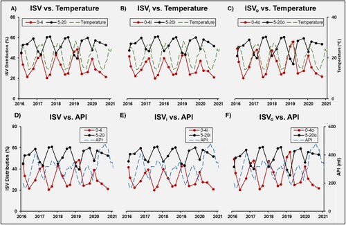
In contrast, API has a weak positive relationship with ISV, particularly for ISV between 5–20, as shown in Figure 6(D). API is usually high during September and October, which coincides with months of high ISV 5–20. When API is high, grass growth is fast, and this leads to high ISV. Low times of API are usually in March and April, which are also part of the trough months of 5–20. This weak relationship between API and ISV is supported by Figure 6(E,F), which compares API to ISV within and outside of 1000 m of residential lands. Overall, temperature has a much stronger relationship and effect on ISV than API.

3.5. Relationship between ISV and its impact factors

This section further explores how strongly ISV are correlated to temperature and API. As for distance to residential lands, observation and analyses has been made for ISV outside of and within 1000 m of residential lands. Correlation test is unnecessary for the ISV and distance as explained earlier in methodology section.

Further analysis is conducted to determine which temperature or precipitation has a greater impact, as Figure 6 reveals the existence of relationships between ISV and these variables. To investigate how much temperature and precipitation relates to ISV, a correlation test of these two variables against ISV is performed. The results are shown in Table 3.

Table 3. Correlation test – ISV vs. temperature and API.

ISV	Temperature	API
0–4	0.804	−0.601
0–4i	0.791	−0.587
0–4o	0.807	−0.614
5–20	−0.664	0.524
5–20i	−0.653	0.482
5–20o	−0.672	0.565

The correlation test (Table 3) shows ISV between 0–4 are highly positively correlated with temperature and moderately negatively correlated with API. ISV between 5–20 are negatively moderately correlated to temperature and positively moderately correlated with API. In comparison, temperature has more influence on ISV than precipitation.

After analyzing distance, temperature and API, Table 4 summarizes the relationship between ISV and these three impact factors. Table 4 shows when ISV is low, there is a negative correlation with precipitation, and a positive correlation with distance and temperature, and vice versa when ISV is high. Therefore, the necessity of using high SR data increases when grasslands are closer to the city, temperature is lower, and precipitation is heavier.

Table 4. Relationship between ISV and three factors. ↑ = increase, ↓ decrease, + positive, − negative.

Impact factors	Scenario	Inter-satellite variability (ISV)
		0–4 (low ISV)	Relationship	5–20 (high ISV)	Relationship
Distance to residential land	Closer	↓	+	↑	−
	Farther	↑		↓
Temperature	Lower	↓	+	↑	−
	Higher	↑		↓
API	Less	↑	−	↓	+
	Heavier	↓		↑

From previous discussion and analysis, temperature has the most effect on ISV because it is dependent on the seasonality and grasslands’ growth varies depends on the season. Precipitation also has a slight influence on ISV. When precipitation increases, the percentage of high ISV also increases. This is because actively growing grass is more challenging to assess especially in combination with precipitation that promotes grass growth. This further complicates the process of observing and measuring GCD using remote sensing techniques.

There is also a significant difference in ISV when distance to residential lands is less than 1000 m. This is because the pixel observed by the satellite might be covering different land features thus decreasing the ability calculate GCD correctly.

4. Conclusion

This study utilizes remote sensing data from Landsat 8 (higher resolution) and MODIS (relatively lower resolution) satellites to estimate GCD and calculate ISV from 2016 to 2020. The research reveals that GCD generated from different SR remote sensing satellite data exhibit discrepancies that vary in space and over time. The higher the ISV, the higher the need to use high SR remote sensing data for grassland observation and monitoring.

This research examines three impact factors: distance, temperature and precipitation to represent location, season and weather respectively. By collecting the data of these three impact factors from 2016 to 2020, and analyzing the characteristics of the changes between ISV and the three impact factors, the relationships between ISV and three impact factors are revealed and summarized as following:

• The relationships between ISV and impact factors are different between low ISV (0–4) and high ISV (5-20); the impact factors with positive correlation to ISV when ISV is low will develop into negative correlation when the value of ISV becomes high, and vice versa.

• ISV is higher for grasslands located within 1000 meters of residential areas than those outside. Temperature exhibits a strong positive correlation with ISV when ISV is low and a moderate positive correlation when ISV is high. Precipitation exhibits a moderate negative correlation when ISV is low and positive correlation when ISV is high. Temperature has a greater influence on ISV than precipitation.

• High SR remote sensing data should be used in regions near cities or residential areas with diverse and complex land cover. The need for high SR data increases during winter and rainy seasons.

These findings can help decision-makers in fire monitoring make informed decisions about when and where to use specific SR satellite data for grassland fire monitoring in an environmental context.

Comparing with other grassland fire monitoring methods, satellite remote sensing technology has great advantages in terms of efficiency and effectiveness, and it has been widely applied in the field of environment protection and observation, especially in grassland fire monitoring. Studying the characteristics and exploring the relationships between ISV and its impact factors can help to provide guidance on how to balance accuracy and cost when developing a grassland fire monitoring strategy and implementation plan.

According to the research results of this study, the following recommendations can be drawn. Satellite remote sensing technology offers efficient and effective methods for monitoring grassland fires. To achieve the highest level of accuracy, it is recommended to use higher SR remote sensing satellite data when possible. Additionally, the choice of satellite data with different SRs should be based on the magnitude of the ISV at different times and regions. For example, Sentinel 2 should be used in areas where the majority of ISV are high (5–20), while Landsat 8 should be used in areas where the high ISV (5–20) is more than the low ISV (0–4). MODIS is recommended for areas where the majority of ISV are low (0–4). When time, labor and economic resources are limited, it is advised to use high SR remote sensing satellites only in high ISV areas. These high SR data should be used in regions close to cities or with complex land covers, during seasons with low temperature such as winter, late autumn or early spring, and during rainy seasons when precipitation is high. In addition, it is worth noting that, high ISV predominate in winter and spring, which means that the use of higher SR satellites can notably improve the monitoring effect. However, in summers and autumns, the proportion of high ISV is relatively small, this indicates that using higher SR satellite data to improve grassland fire monitoring is minuscule. From the perspective of satellite monitoring, the necessity of using higher SR satellite during these two seasons is less. However, considering that the temperature is relatively high in summer and autumn, and the climate is relatively arid, these are natural conditions make grasslands more prone to fire. Therefore, the usage of higher SR satellites for grassland fire monitoring in summers and autumns should be based on realistic situational needs.

Future research could expand the data coverage to the entire state of Victoria or the whole of Australia with extended observation time frame and use additional methods to eliminate cloud interference such as radar, and add the latest satellite data that replace MODIS such as VIIRS. Additionally, GCD calculation formula can be adjusted to satellite sensors and more localized regions. Additional impact factors could be identified to test and analyze the correlation of GCD and ISV. Predicting the future Grassland Fire Danger Index trend using GCD as the main index could be explored. Maps could be developed for end-user for each season, outlining areas with appropriate need for different SR satellite monitoring, constructing maps for where higher SR satellite data should be used, and what level of grassland fire monitoring is required could also be undertaken. This future work could result in the most efficient Australian national grassland fire monitoring system using appropriate SR satellite data for environmental protection. Such a system could provide the basis for a global network devoted to grassland fire monitoring and its impact on the environment, using remote sensing satellite technology.

Acknowledgements

I would like to thank Dr. Nigel Tapper, Dr. Sarah Harris, Dr. Christoph Rüdiger, and Dr. Xuan Zhu for their comments and feedbacks during my research. Thanks also go to the Monash University for providing Monash Graduate Scholarships (MGS). I would also like to extend my gratitude to the School of Science, University of New South Wales for the Research Support Funds 2022/2023 and facilitating a healthy research environment during the development of this manuscript.

Disclosure statement

No potential conflict of interest was reported by the author(s).

Additional information

Funding

This work was supported by Monash University and University of New South Wales Canberra.

References

- Brigitte, Leblon, Bourgeau-Chavez Laura, and San-Miguel-Ayanz Jesús. 2012. “Use of Remote Sensing in Wildfire Management.” In Sustainable Development, edited by Curkovic Sime, 55–57. Rijeka: IntechOpen.
- Calkins, Keith G. 2005. “Correlation Coefficients.” Accessed December 11. https://www.andrews.edu/~calkins/math/edrm611/edrm05.htm
- Chuvieco, Emilio, Inmaculada Aguado, Javier Salas, Mariano Garcia, Marta Yebra, and Patricia Oliva. 2020. “Satellite Remote Sensing Contributions to Wildland Fire Science and Management.” Review of Current Forestry Reports 6 (2): 81–96. https://doi.org/10.1007/s40725-020-00116-5
- Department of Jobs, Precincts and Regions. 2018. “Victorian Land Use Information System 2016-2017.” https://discover.data.vic.gov.au/dataset/victorian-land-use-information-system-2016-2017.
- Emergency Management Australia, Australasian Fire Authorities Council, and Country Fire Authority. 2000. Wildfire Prevention in Australia. Date accessed: 2023 1–5. Dickson ACT 2602, Australia: Department of Defence.
- European Space Agency. 2021. “Radiometric Resolutions.” https://dragon3.esa.int/web/sentinel/user-guides/sentinel-2-msi/resolutions/radiometric#:~:text=Radiometric%20resolution%20is%20the%20capacity,of%208%20to%2016%20bits.
- Fontana, Denise. 2014. “Case Study for the CFA Grassland Curing and Fire Danger Rating Project.” Publisher: Country Fire Authority. https://www.bushfirecrc.com/sites/default/files/managed/resource/case_study_grasslands_final_report.pdf
- Forest Management Victoria. 2021. “Past Bushfires.” Accessed November 12. https://www.ffm.vic.gov.au/history-and-incidents/past-bushfires.
- Gullan, Paul. 2021. “Victorian Ecosystems.” Accessed November 12. http://www.viridans.com/ECOVEG/grassland.htm.
- Li, Sike. 2020. “Analysis of Landsat 8 Detection of the Interannual Variability of Grassland Curing in Greater Melbourne, Australia.” Review of International Journal of Digital Earth 13 (11): 1321–1338. https://doi.org/10.1080/17538947.2019.1710273.
- Li, Sike. 2021. “Inter-satellite Variability of Grassland Curing Maps Produced by Different Satellite Sensors – Victoria, Australia.” Review of International Journal of Digital Earth 14: 1–22. https://doi.org/10.1080/17538947.2021.1900938.
- Li, Xungui, Yining Wei, and Fang Li. 2021. “Optimality of Antecedent Precipitation Index and its Application.” Review of Journal of Hydrology 595: 126027. https://doi.org/10.1016/j.jhydrol.2021.126027.
- Maestrini, Bernardo, and Bruno Basso. 2018. “Predicting Spatial Patterns of Within-Field Crop Yield Variability.” Review of Field Crops Research 219: 106–112. https://doi.org/10.1016/j.fcr.2018.01.028.
- National Aeronautics and Space Administration. 2021a. "LANDSAT 8." Accessed August 18. https://landsat.gsfc.nasa.gov/landsat-8/landsat-8-overview
- National Aeronautics and Space Administration. 2021b. “MODIS Specifications.” Accessed February 21. https://modis.gsfc.nasa.gov/about/specifications.php
- National Aeronautics and Space Administration. 2021c. "LANDSAT 8 MISSION DETAILS." Accessed August 18. https://landsat.gsfc.nasa.gov/satellites/landsat-8/landsat-8-mission-details/
- Sharma, Sonisa, and Kundan Dhakal. 2021. “Boots on the Ground and Eyes in the Sky: A Perspective on Estimating Fire Danger from Soil Moisture Content.” Review of Fire 4 (3): 45. https://doi.org/10.3390/fire4030045
- US Geological Survey. 2020. “Landsat 8 Collection 1 (C1) Land Surface Reflectance Code (LaSRC) Product Guide.” In.: Department of the Interior, US Geological Survey, USGS Press Reston, VA, USA.
- Vermote, Eric. 2015. “MOD09A1 MODIS/Terra Surface Reflectance 8-Day L3 Global 500 m SIN Grid V006.” NASA EOSDIS Land Processes DAAC, Accessed October 25. https://doi.org/10.5067/MODIS/MOD09A1.006
- Wang, Zhaobin, Yikun Ma, Yaonan Zhang, and Jiali Shang. 2022. “Review of Remote Sensing Applications in Grassland Monitoring.” Review of Remote Sensing 14 (12): 2903. https://doi.org/10.3390/rs14122903
- Xie, Wen-ping, and Jing-song Yang. 2013. “Assessment of Soil Water Content in Field with Antecedent Precipitation Index and Groundwater Depth in the Yangtze River Estuary.” Review of Journal of Integrative Agriculture 12 (4): 711–722. https://doi.org/10.1016/S2095-3119(13)60289-0.
- Zhao, Shaohua, Qiao Wang, Ying Li, Sihan Liu, Zhongting Wang, Li Zhu, and Zifeng Wang. 2017. “An Overview of Satellite Remote Sensing Technology Used in China’s Environmental Protection.” Review of Earth Science Informatics 10 (2): 137–148. https://doi.org/10.1007/s12145-017-0286-6