Optimizing satellite ground station facilities scheduling for RSGS: a novel model and algorithm

ABSTRACT

As the rapid increasing of the number of the satellites, the number of facilities of the satellite ground stations is becoming insufficient and the conflicts of serving satellite data missions exist. To make full use of the facilities of the China Remote Sensing Satellite Ground Station (RSGS), scheduling optimization of these facilities was studied in this paper, which was not well-solved by the original method in the operation system of RSGS. The problem is formulated as a continuous time-based mixed integer linear programming (MILP) model. A decomposition optimization algorithm is proposed to solve the large-scale problem, which is difficult to solve using traditional methods. In the first step, the particle swarm optimization (PSO) algorithm is used to optimize the multi-ground station relay tasks, and the multi-ground station optimization problem is transformed into several single ground station optimization problems. Next, in two additional steps, optimization of the facilities at a single ground station is performed to further reduce the size of the model. The proposed method has been applied to operations systems of RSGS, and the approach presented in this article has demonstrated stable performance and sufficient efficiency online, resulting in the automation of facility scheduling.

KEYWORDS:

• Facility scheduling
• decomposition algorithm
• satellite ground station

1. Introduction

The China Remote Sensing Satellite Ground Station (RSGS) is one of the largest ground station networks in the world and consists of several ground stations located both inside and outside China. RSGS receives data from more than 300 missions per day, including TT&C (telemetry, tracking, and command) and DT (data transmission) missions, and more than 10⁷ GB of downloaded data per year in total. The number of missions has increased dramatically along with the number of satellites, and the RSGS facilities (including antennas, recorders, and demodulators) with complex connections between them are now considered insufficient. The scheduling of ground stations facilities is an effective way to improve the utilization of ground facilities and ensure the timeliness of data acquisition.

1.1. Problem statement

The processes that occur at a satellite ground station network are illustrated in Figure 1. Satellites missions can be categorized into three types: DT missions, TT&C missions, and missions that involve both TT&C and DT. DT missions require the use of receiving facilities (antennas), recording facilities (recorders), and connection facilities (demodulators, etc.). The facilities used for TT&C missions include antennas and the necessary accessories; this means that antennas are the only facilities considered in the scheduling of TT&C missions. The relationship between satellite missions, antennas, recorders, and demodulators corresponds to a many-to-many mapping, as shown in Figure 2. From the perspective of scheduling optimization, satellite missions involve multiple ground stations, and many parallel facilities are involved in each process. Coupled connections also exist between facilities, which means that large, complex models are required to represent these relationships.

Figure 1. Illustration of the processes that take place at a satellite ground station network.

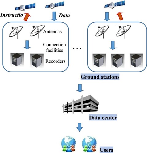
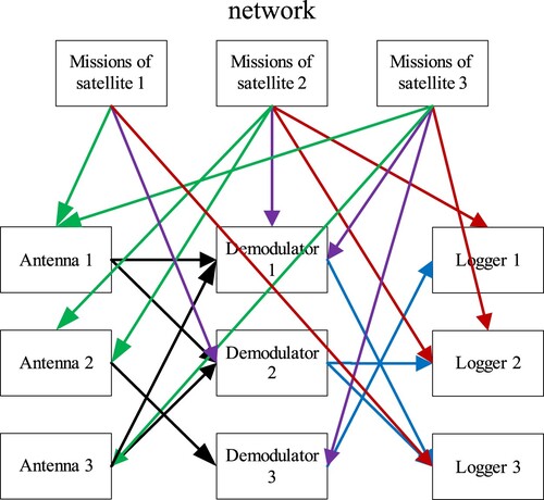
Figure 2. Map of the relationships between missions and facilities.

Notes: The green lines denote the available connections between satellites and antennas; the purple lines denote the available connections between satellites and demodulators; the red lines denote the available connections between satellites and loggers; the black lines denote the available connections between antennas and demodulators; the blue lines denote the available connections between demodulators and loggers.

During the 36 years which the RSGS has been constructed, facilities with different capabilities have been added and developed. Because of this, and because the relationships between antennas, demodulators, and recorders are complex, in order to make full use of all of the facilities and achieve automatic scheduling, it is necessary to study the overall process scheduling and take into account the differences in performance of parallel facilities and the connections between all of the different types of facilities at the ground stations.

1.2. Summary of research

There have been many studies that have considered the ground station scheduling problem (Petelin, Antoniou, and Papa 2021; Spangelo et al. 2015; Xhafa and Andrew 2021). Xhafa and Andrew (2021) reviewed the state of the art in the satellite scheduling problem, analyzed the mathematical formulations and meta-heuristics solving methods. Petelin, Antoniou, and Papa (2021) solved a number of benchmark static instances of the ground scheduling problem with six different evolutionary multi-objective algorithms (NSGA-II, NSGA-III, SPEA2, GDE3, IBEA, and MOEA/D). Spangelo et al. (2015) developed models and algorithms for solving the single-satellite, multi-ground station communication scheduling problem, with the objective of maximizing the total amount of data downloaded from space. However, most of these studies focused on one or more sub-processes related to DT or TT&C processes, such as antenna scheduling or recorder scheduling. In relation to antenna scheduling, Ko (2016) considered the scheduling of ground station facilities with multiple antennas where the objective was to maximize the data transmission and the constraints included the antenna switching time. Marinelli et al. (2011) studied the problem of data exchange between ground stations and the Galileo satellite constellation. The problem was treated as a multiple processor scheduling problem and was solved by Lagrangian relaxation combined with a heuristic method. Similarly, Lin et al. (2003) considered a low-orbit earth observation satellite mission scheduling problem, and Lagrangian relaxation and linear search techniques were adopted to solve this problem. Falone and Corrao (2018) proposed a multi-stage strategy algorithm for the ground station scheduling problem, and methods such as genetic algorithms, graph theory, and linear programming were combined for solution. Antennas allocation were considered in the ground station resource scheduling. Li, Zhang, et al. (2015) considered the multiple antenna scheduling problem; however, the differences in proprieties and performance of the different antennas were not considered in this study. Song et al. (2022) investigated collaborative satellite–ground observation planning and proposed the use of an improved artificial bee colony algorithm and a satellite–ground resource coordinated time-selection algorithm. Similarly, An et al. (2021) discussed the optimal strategy for antenna scheduling at four ground stations, each of which had a single antenna. Based on the requirements of ESA, Xhafa, Herrero, et al. (2013) proposed applying a Struggle Strategy Genetic Algorithm (SSGA) to the ground station scheduling problem and produced results related to the scheduling of both single and multiple ground stations. The objective was to maximize the service provided for missions and the use of ground station antennas. Different to the situation at the RSGS (where multiple ground stations deal with multiple satellite missions), each satellite was considered to interact with a specific ground station and each ground station only served one mission at a time (Xhafa et al. 2012, Xhafa, Barolli, et al. 2013). A Constraint Satisfaction Problem (CSP) model of the detection satellite data exchange was formulated, in which all of the facilities at a single ground station are seen as one set of equipment so that constraints imposed by the ground facilities do not need to be considered. Zhang et al. (2019) and Wang, Zhang, and Chen (2019) represented the ground station scheduling problems by a multiple-objective CSP model, but the scheduling of demodulators and recorders was not considered.

Decomposition strategy can be used to solve large-scale scheduling problems, especially when the different types of variables can be optimized in different levels (Zhang et al. 2016). Based on the decomposition framework, the hybrid algorithm with various subalgorithms used for two-step optimization has been studied (Yan et al. 2021). Different hybrid algorithms with meta-heuristics and exact methods employed were developed for large-scale scheduling problems (Falone and Corrao 2018). Meta-heuristics which include genetic algorithm (Li, Wang, et al. 2015; Sun and Xhafa 2011; Xhafa et al. 2012; Xu et al. 2020), particle swarm optimization (PSO) (Fan et al. 2022), ant colony optimization (Iacopino et al. 2014), and cuckoo search algorithm (X. Li et al. 2023), are effective for problems with large search spaces and can provide satisfactory solutions in reasonable time frames. However, the quality of solutions cannot be guaranteed, and complex constraints can be challenging to represent using meta-heuristic methods. Meanwhile, exact algorithms, such as the dual simplex method for linear programming (LP) models, the interior point method for NLP models, the branch-and-bound method for mixed integer linear programming (MILP) models, and the outer approximation method for mixed integer nonlinear programming (MINLP) models, can produce optimum solutions, but low-quality final solutions may be possible with insufficient computational time. As such, a hybrid algorithm combining meta-heuristics and exact methods is preferred to solve scheduling problems (Harjunkoski et al. 2014).

Genetic algorithm (GA) is a widely used metaheuristic optimization algorithm based on the principles of natural selection and genetics. GA is known for its ability to find global optima in complex search spaces, especially with large numbers of variables or constraints. However, the quality of solutions cannot be guaranteed, and complex constraints can be challenging to represent using meta-heuristic methods (Goldberg 1989). Linear programming (LP) solvers are computational tools used to optimize problems through mathematical modeling. LP solvers have both free open-source versions and commercial versions that are widely used in different fields and application scenarios. Open-source LP solvers have the advantage of being free and open to customization, making it easier for users to modify codes according to their unique requirements. These solvers are compatible with various programming languages and computing environments. In this paper, we use the open-source COIN CLP/CBC solver, which is a high-performance solver for linear, mixed-integer, and constraint programming. COIN CLP/CBC is provided by Google, supports Python and C++, and is extensively used in finance, logistics, and manufacturing.

1.3. Previous method used in RSGS

The scheduling problem of RSGS was first time solved by a genetic algorithm (Shang et al. 2014). However, there was a definite gap between the results that were obtained using this approach and the demands of real situations. The optimization algorithm did not perform well, and the scheduling results still needed manual adjustment to provide accurate ground station arrangements (Tian et al. 2020). The purpose of scheduling in this study is to realize automatic management of the operation of the RSGS. To the best of the author’s knowledge, there have been no published studies in which the connection between the facilities involved in each sub-process was considered. However, because of the cost of manual operations and because of high computation efficiency requirements, optimization of the overall scheduling needs to be considered in the case of multi-ground station network with parallel facilities so that automatic scheduling can be realized. But the complexity of this problem makes it difficult to model and solve. In particular, the following problems are encountered: (1) the complexity of the processes and the scheduling rules make the modeling difficult, and (2) the existence of multiple parallel facilities and the complex mapping relationships between these facilities lead to a large quantity of binary variables. As a result, the problem is difficult to solve efficiently for real cases.

The rest of the paper is organized as follows. The scheduling model formulation is explained in section 2. On the basis of the process analysis, the decomposition approach to solve the problem is presented in section 3. In section 4, comparisons with the original method used for the operating system at RSGS are provided to illustrate the effectiveness of the proposed method for several well-designed cases. Conclusions are drawn in section 5.

2. Scheduling model formulation

2.1. Problem statement

In this paper, the problem of the scheduling of satellite ground station facilities is considered.

The data communication between satellites and ground stations is depicted in Figure 1, and the problem can be stated as follows.

Given the following:

1. a set of ground stations belonging to the RSGS ground station network

2. a set of satellites that the RSGS serves

3. ground station facilities including antennas, demodulators, and recorders at each ground station

4. information of missions, and involving mission types, satellites, priorities, beginning and end time; and target ground stations, in particular relay missions involving several ground stations

5. the mapping relationships between all of the facilities, including available satellite–antenna, satellite–recorder, satellite–demodulator, antenna–demodulator, and recorder–demodulator matrices

6. differences in priority resulting from differences in performance (see Table 1), as well as the satellite–antenna and satellite–recorder priority matrices

7. the possibility that different missions of the same satellite can have different code rates and the using of recorders and demodulators is constricted by these rates, meaning that the upper and lower bounds of these rates for recorders and demodulators are required.

Table 1. Prioritization of available facilities, showing the weights assigned to different facilities.

Mission/facility	Facility 1	Facility 2	Facility 3
Mission 1	1	0	Null
Mission 2	1	Null	0
Mission 3	0	1	2

Notes: The values indicate the priority given to the facility for the mission. A smaller value means a higher priority. ‘Null’ denotes that the facility is not available for the mission.

The goal is then to determine the following:

1. which facility is used to serve which mission

2. whether the mission is fully served or not. The beginning and end times of missions can be adjusted if the facilities are too busy to serve all of the missions.

To better formulate real-world satellite DT and TT&C processes, several reasonable descriptions are made as follows.1.

a.	All the processes are considered to be continuous.
b.	Antennas, recorders, and demodulators are considered in the case of DT processes, and a mission can be served by all three types of these facilities. Antennas are considered in the case of TT&C processes. Missions including both DT and TT&C processes are considered to consist of two separate missions.
c.	The difference in the performance of facilities and load balancing is considered: the facilities available for a mission should be arranged so that the facilities that perform better are given preference. Facilities that perform equally well should be given equal preference (see Table 1).

To realize the load balancing for the facilities, a random number $n_{s,f}$, whose values are uniformly distributed, is then added to the priority weight, $p_{s,f}$ ($s$ denotes the mission and $f$ denotes the facility), as shown in Table 2. This means that facilities shown as having the same priority in Table 1 get equal use.

d.

Natural features and buildings can block the transmission of satellite data. The orientation of the facilities during the DT and TT&C processes should be considered so that the possibility of those facilities being occluded can be avoided. Offline computations are regularly run to determine whether the signal is occluded or not during the mission to improve the computational efficiency. The weights of signal confliction of missions are computed as follows: If signal occlusion occurs, the length of confliction time is obtained before the facilities scheduling. A penalty value for the confliction time, $sh{l}_{s,f}$($s$ denotes the mission and $f$ denotes the facility), is added to the priority value in Table 2 to avoid the use of the occluded facility (see Table 3).

Table 2. Improved prioritization of facilities with load balancing considered.

Mission/facility	Facility 1	Facility 2	Facility 3
Mission 1	1+$n_{11}$	$n_{12}$	Null
Mission 2	1+$n_{21}$	Null	$n_{23}$
Mission 3	$n_{31}$	1+$n_{32}$	2+$n_{33}$

Note: $n_{s,f}$ is small compared to $p_{s,f}$, approximately10 times smaller.

Table 3. Improved facility prioritization with load balancing and signal confliction considered.

Mission/facility	Facility 1	Facility 2	Facility 3
Mission 1	1+$n_{11}$+$sh{l}_{11}$	$n_{12}$+$sh{l}_{12}$	Null
Mission 2	1+$n_{21}$+$sh{l}_{21}$	Null	$n_{23}$+$sh{l}_{23}$
Mission 3	$n_{31}$+$sh{l}_{31}$	1+$n_{32}$+$sh{l}_{32}$	2+$n_{33}$+$sh{l}_{33}$

2.2. Constraints

It should be noted that the multi-ground station scheduling problem involves relay tasks, which is discussed in Section 3.1. The method presented in Section 3.1 transforms the multi-ground station scheduling problem into multiple single-ground station scheduling problems. The model constraints for the single-ground station scheduling problem are presented in this section, while the objective function of this problem is introduced in Section 2.3.

The model for the data reception and TT&C processes is described in Section 2.2.1 below. The constraints that apply to the data recording process are described in Section 2.2.3. Facilities such as modulators and the facility connection matrix are simplified to demodulators, and their modeling is described in Section 2.2.2.

2.2.1. Constraints on data reception and TT&C processes

(1)

Each mission should be served by one antenna. If there are not enough antennas to serve all missions, mission $i$ may not be served: (1) $\sum _{j\in J}an{t}_{ij}\le 1,\mathrm{\forall }i\in I$(1)

(2)

Each antenna can only serve one mission at the same time. Moreover, antennas have a switching time, $\tau$. That is, antenna $j$ cannot serve mission $i^{\mathrm{\prime }}$ within a time $\tau$ after the completion of the previous mission (mission $i$). If there are not sufficient antennas to serve all missions completely, the beginning or end time of some missions can be changed to reduce the mission time. This means that the beginning time of mission $i$($b_i$) and the end time of mission $i$($c_i$) should be considered to be continuous variables. Equation denotes the scenario that mission $i\mathrm{\prime }$ is later than mission $i$ and the two missions use the same antenna. So $b_{i^{\mathrm{\prime }}}$ should be later than $c_i$, and the switching time $\tau$ is required between the missions: (2) $b_{i^{\mathrm{\prime }}}\ge c_i+\tau -M(1-or{d}_{i{i}^{\mathrm{\prime }}})-M(2-an{t}_{ij}-an{t}_{i^{\mathrm{\prime }}j}),\mathrm{\forall }i,i^{\mathrm{\prime }}\in I,i^{\mathrm{\prime }}>i,j\in J$(2)

While Equation (3) denotes the scenario that mission $i^{\mathrm{\prime }}$ is earlier than mission $i$ and the two missions use the same antenna. So $b_i$ should be later than $c_{i^{\mathrm{\prime }}}$, and the switching time $\tau$ is required between the missions. (3) $b_i\ge c_{i^{\mathrm{\prime }}}+\tau -M\ast or{d}_{i{i}^{\mathrm{\prime }}}-M(2-an{t}_{ij}-an{t}_{i^{\mathrm{\prime }}j}),\mathrm{\forall }i,i^{\mathrm{\prime }}\in I,i^{\mathrm{\prime }}>i,j\in J$(3) Here $or{d}_{i{i}^{\mathrm{\prime }}}$ is an intermediate variable that denotes the order of mission $i$ and mission $i^{\mathrm{\prime }}$: $or{d}_{i{i}^{\mathrm{\prime }}}=1$ denotes that the beginning time of mission $i$ is earlier than that of mission $i^{\mathrm{\prime }}$. (4) $or{d}_{i{i}^{\mathrm{\prime }}}>{\displaystyle \frac{1}{M}(b_{i^{\mathrm{\prime }}}-b_i)}$(4) and (5) $1-or{d}_{i{i}^{\mathrm{\prime }}}>{\displaystyle \frac{1}{M}(b_i-b_{i^{\mathrm{\prime }}})}$(5) where $M$ denotes a positive number, and M = 10⁶ here.

The beginning and end time of mission $i$ should be within the time range during which the satellite is visible from the ground station. That is, the beginning time of mission $i$ should be later than the begin time of the visible range: (6) $b_i\ge s{t}_i$(6)

And the end time of mission $i$ should be earlier than the end time of the visible range, (7) $c_i\le t{e}_i$(7) where $s{t}_i$ and $t{e}_i$ are, respectively, the beginning and end of this visible time range for mission $i$.

The beginning time of mission $i$ should be later than the end time: (8) $b_i\le c_i$(8)

(3)	If the time for which a mission lasts is 0, there is no need to arrange an antenna to serve it. If the mission lasts for a time greater than 0, it will be served by an antenna: (9) $\sum _{j\in J}an{t}_{ij}\le c_i-b_i,\mathrm{\forall }i\in I$(9) (10) $\sum _{j\in J}an{t}_{ij}\ge {\displaystyle \frac{1}{M}(c_i-b_i),\mathrm{\forall }i\in I}$(10)
(4)	An antenna can serve DT and TT&C missions of the same satellite at the same time. Such missions are considered to belong to a single mission group: (11) $an{t}_{ij}=an{t}_{i^{\mathrm{\prime }}j},ifGrou{p}_i=Grou{p}_{i^{\mathrm{\prime }}}$(11) where $Grou{p}_i$ is the group to which mission $i$ belongs.

2.2.2. Constraints on demodulators

As the relationships between antennas, recorders, and demodulators correspond to many-to-many mappings, the demodulators need to be considered in the scheduling to avoid an unfeasible scheduling result caused by a lack of connection between facilities.

1. The number of demodulators serving mission $i$ should not be more than the number of channels, $chan{l}_i$. If there are not sufficient facilities to serve all missions, mission $i$ may not be served: (12) $\sum _{g}dem{o}_{ig}\le chan{l}_i$(12) where $dem{o}_{ig}$ is a binary variable. $dem{o}_{ig}=1$ denotes that mission $i$ is served by the demodulator $g$.

2. A demodulator can only serve one channel of a mission at the same time. Equation (13) denotes that the channel $g$ serves mission $i$ and mission $i^{\mathrm{\prime }}$ at the same time and mission $i^{\mathrm{\prime }}$ is later than mission $i$. So $b_{i^{\mathrm{\prime }}}$ should be later than $c_i$, and the switching time $\tau$ is required between the missions. (13) $b_{i^{\mathrm{\prime }}}\ge c_i+\tau -M(1-or{d}_{i{i}^{\mathrm{\prime }}})-M(2-dem{o}_{ig}-dem{o}_{i^{\mathrm{\prime }}g}),\mathrm{\forall }i,i^{\mathrm{\prime }}\in I,i^{\mathrm{\prime }}>i,g\in G$(13) while Equation (14) denotes that the channel $g$ serves mission $i$ and mission $i^{\mathrm{\prime }}$ at the same time and mission $i^{\mathrm{\prime }}$ is earlier than mission $i$. So $b_i$ should be later than $c_{i^{\mathrm{\prime }}}$, and the switching time $\tau$ is required between the missions. (14) $b_i\ge c_{i^{\mathrm{\prime }}}+\tau -M\ast or{d}_{i{i}^{\mathrm{\prime }}}-M(2-dem{o}_{ig}-dem{o}_{i^{\mathrm{\prime }}g}),\mathrm{\forall }i,i^{\mathrm{\prime }}\in I,i^{\mathrm{\prime }}>i,g\in G$(14)

3. There are constraints on the connections between antennas, demodulators, and recorders. If demodulator $g$ is not connectable to the used antenna $j$, it cannot serve mission $i$; if demodulator $g$ is not connected to the used recorder $k$, it cannot be arranged to serve mission $i$: (15) $dem{o}_{ig}\le Alin{k}_{jg}\ast an{t}_{i,j}$(15) (16) $dem{o}_{ig}\le Rlin{k}_{kg}\ast re{c}_{i,k},$(16) where $Alin{k}_{jg}$ is a binary parameter. $Alin{k}_{jg}=1$ denotes that antenna $j$ is connectable to facility $g$. $Rlin{k}_{kg}$ is another binary parameter; $Rlin{k}_{kg}=1$ denotes that recorder $k$ is connectable to facility $g$.

2.2.3. Constraints of recording process

1. If a mission is not served by an antenna, then a recorder is not needed: (17) $\sum _{j\in J}an{t}_{ij}\le \sum _{k\in K}re{c}_{ik},\mathrm{\forall }i\in I$(17)

2. To avoid operation risks in the data recording process, it is necessary to minimize the number of missions being served by any one recorder at the same time. The number of missions using recorder $k$ at the same time as mission $i,z_{ik}$, is defined as (18) $\sum _{i\in Inj{a}_i}re{c}_{i^{\mathrm{\prime }}k}\le z_{ik},\mathrm{\forall }i,i^{\mathrm{\prime }}\in I,i^{\mathrm{\prime }}>i,k\in K$(18) where $Inj{a}_i$ denotes the missions that overlap with mission $i$ as the situation where recorders serve multiple missions at the same time only occurs in the case of a time-overlapping mission set.

3. There are channel constraints on recorders. The total number of channels used by the missions served by the recorder $k$ at the same time should be no greater than the number of recorder k’s channels ($nu{m}_k$): (19) $\sum _{i^{\mathrm{\prime }}\in I}(y_{i{i}^{\mathrm{\prime }}}\ast chan{l}_{i^{\mathrm{\prime }}})+chan{l}_i-nu{m}_k\le M(1-re{c}_{ik}),\mathrm{\forall }i\in I,k\in K$(19) Here $nu{m}_k$ denotes the number of recorder k’s channels, and $y_{i{i}^{\mathrm{\prime }}}$ is a binary variable. $y_{i{i}^{\mathrm{\prime }}}=1$ denotes that the time interval between missions $i$ and $i^{\mathrm{\prime }}$ is smaller than the recorder switching time; that is, if $b_{i^{\mathrm{\prime }}}\ge c_i+\tau$, then $y_{i{i}^{\mathrm{\prime }}}=0$, as shown in Equation (20): (20) $b_{i^{\mathrm{\prime }}}+(p{t}_i+\tau )\ast y_{i{i}^{\mathrm{\prime }}}\ge c_i+\tau -M(2-re{c}_{ik}-re{c}_{i^{\mathrm{\prime }}k})-M(1-or{d}_{i{i}^{\mathrm{\prime }}}),\mathrm{\forall }i,i^{\mathrm{\prime }}\in I,i^{\mathrm{\prime }}>i,k\in K$(20)

4. There are constraints on the code rates of recorders. The code rate of satellite data cannot be greater than that of the recorder: (21) $\sum _{i^{\mathrm{\prime }}\in I}(y_{i{i}^{\mathrm{\prime }}}\ast rat{e}_{i^{\mathrm{\prime }}})+rat{e}_i-trat{e}_k\le M(1-re{c}_{ik}),\mathrm{\forall }i\in I,k\in K$(21) where $trat{e}_k$ denotes the rate of recorder $k$; $rat{e}_i$ denotes the rate of mission $i$. If mission $i$ has multiple channels, $rat{e}_i$ denotes the rate of the channel with the highest rate.

5. Recorders are not needed for TT&C missions: (22) $\sum _{k\in K}re{c}_{ik}\le 0,\mathrm{\forall }i\in I^{up}$(22) $I^{up}$ denotes the set of TT&C missions.

2.3. Objective

The aim of the facilities scheduling is to allow as many DT and TT&C missions as possible to be completed: that is, to minimize the penalty for the unserved missions. This penalty includes (1) a penalty related to the antenna arrangement for the mission, denoted by $C_1$ in Equation (23); (2) a penalty related to the demodulator arrangement, denoted by $C_2$ in Equation (24); (3) a penalty related to the recorder arrangement, denoted by $C_3$ in Equation (25): (23) $C_1=\sum _{i\in I}p{a}_i^1\ast \left(1-\sum _{j\in J}an{t}_{ij}\right)+\sum _{i\in I}p{a}_i^2\ast ma{t}_i+\sum _{i\in I}\sum _{j\in J}w{a}_{ij}\ast an{t}_{ij}$(23) (24) $C_2=\sum _{i\in I}p{c}_i\ast \left(chan{l}_i-\sum _{g\in G}dem{o}_{ig}\right)$(24) (25) $C_3=\sum _{i\in I}p{r}_i^1\ast \left(1-\sum _{k\in K}re{c}_{ik}\right)+\sum _{i\in I}\sum _{k\in K}w{r}_{ik}\ast re{c}_{ik}+\sum _{i\in I}{z}_{ik}$(25) (26) $C=C_1+C_2+C_3$(26) $C_1$ includes a penalty for not arranging an antenna for the mission (the first term in Equation (23)), a penalty for incompletely serving the mission (the second term), and the sum of the weights of the used antennas (the third term). $p{a}_i^1$ is a parameter denoting a penalty that results if mission $i$ not served by any antenna. Variable $ma{t}_i$ denotes the length of an incomplete mission $i$; parameter $p{a}_i^2$ denotes the penalty of unit incomplete time of mission $i$. Weight $w{a}_{ij}$ denotes the priority given to antenna $j$ serving mission $i$ (see Table 3). $C_2$ is a penalty that results from having insufficient demodulators. Parameter $p{c}_i$ is a penalty that is assigned if no antenna is arranged for mission $i$, denotes the number of channels used in mission, and is a binary variable; denotes that demodulator serves mission. $C_3$ includes a penalty for not arranging a recorder for the mission (the first term of Equation (25)) as well as the sum of the weights of the recorders that are used (the second term).$p{r}_i^1$ is a parameter that gives the penalty for mission $i$ not being served by any recorder. Weight $w{r}_{ik}$ denotes the priority given to recorder $k$ serving mission $i$ (see Table 3). Because of the need to consider the stability of the performance of the facilities, the number of missions using the same recorder at the same time is minimized by the last term of Equation (25).

The objective of the problem is denoted in Equation (27). (27) $minC$(27)

3. Decomposition algorithm

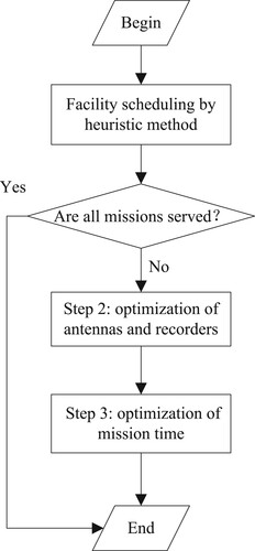
The proposed decomposition algorithm includes the optimization of a multi-ground station facility and two single-ground station facility optimization steps (two MILP subproblems). The flowchart of the proposed decomposition algorithm is shown in Figure 3, where the objectives and the constraints at each step are summarized.

Figure 3. Overall framework of the decomposition algorithm.

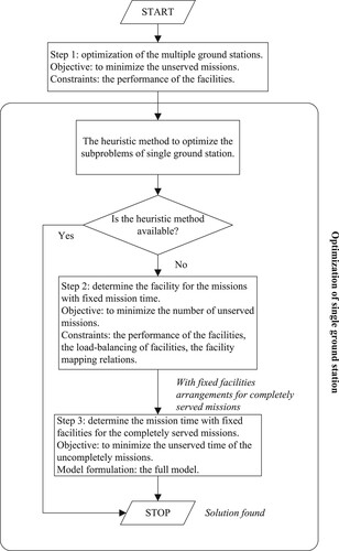
The steps included in the algorithm are as follows.

Step 1: Optimization of relay missions for multiple ground stations. The time range for relay missions covers multiple ground stations, and overlaps exist between the time ranges during which the satellite is visible from these different ground stations (see section 3.1). One group of the facilities at these ground stations is needed to serve the mission during the overlap, considering that the scheduling of facilities at all of the multiple ground stations should be optimized to serve as many missions as possible. The coupling between the facilities at the multiple ground stations is disposed at this step, and the multiple-ground station facility optimization problem is converted to several single-ground station facility optimization problems.

Step 2: Optimization of the facilities at a single ground station: the status of the facilities is optimized.

Step 3: Optimization of the facilities at a single ground station: the beginning and end time of missions is optimized using the information obtained in Step 1 and Step 2.

The above algorithm begins with the optimization of relay missions and involves facilities at multiple ground stations. A simplified scheduling model is formulated and solved by a PSO algorithm. The objective of the model is to minimize the number of unserved missions; that is, the relay mission should be served by a less busy ground station. The size of the model is reduced as the coupling is removed, and the problem is decomposed into several subproblems at this step.

Next, the single-ground station optimization is addressed. When the number of missions that overlap in time is less than the number of available facilities, the problem can be solved by a heuristic method. However, when the problem is more complex, this method is not suitable. Also, after the optimization of the relay missions, the model is often still very large. In particular, if the facilities are too busy to serve all of the missions, the adjustments to the mission time can lead to there being many binary and continuous variables. Thus, the problem is further decomposed into two subproblems. The first problem is to determine which facilities can be used to serve the missions, and the second one is to determine the beginning and end time of the missions if the missions cannot be served completely. Two MILP models are formulated to solve these two subproblems.

The input and output for each step is as follows:

The input of Step 1 includes the information on all the missions and ground stations. Output of Step 1 includes the mapping relationship between missions and ground stations, indicating which ground station serves each mission.

The input of Step 2 includes the missions’ information for each ground station, as well as the information about each ground station. The output of Step 2 is the mission states (whether each mission is served or not) and facility states for each mission (whether the facility is allocated to each mission or not).

The input of Step 3 is the output of Step 2, as well as the input of Step 2. The output of Step 3 includes the beginning and end times of each mission, as well as the facility that will serve each mission.

3.1. Optimization of the scheduling at multiple ground stations (Step 1)

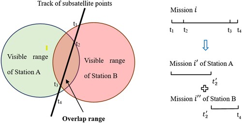
As relay missions are served by more than one ground station and the ranges of these ground stations overlap, the ground station and facilities that serve the mission during each time period need to be determined (see Figure 4(a)). Mission $i$ can be served by both ground station A and ground station B during the time period [t₂, t₃]; this mission is decomposed into mission $i^{\mathrm{\prime }}$ for ground station A and mission $i^{\mathrm{\prime }\mathrm{\prime }}$ for ground station B to avoid duplication as shown in Figure 4(b). The time periods covered by these two missions are [t1, $t_3^{\mathrm{\prime }}$] and [$t_2^{\mathrm{\prime }}$, t4], where $t_2\le t_2^{\mathrm{\prime }}\le t_3$.

Figure 4. (a) Diagram showing the visible range of two ground stations A and B and (b) the decomposition of relay missions.

A simplified model is used to formulate the multi-ground station antenna scheduling for relay missions and a PSO algorithm is proposed to solve the problem.

PSO is a population-based stochastic optimization technique proposed by Kennedy (2005) and Kennedy and Eberhart (1995). Inspired by the social behavior of animals, such as insects, herds, and birds, PSO uses a swarm mode to search a large region in the solution space of the optimized objective function. The particles in the swarm cooperate to find food, and each member constantly adapts its search pattern based on its own and other members’ learning experiences. A key concept in PSO is artificial life, which applies the characteristics of living systems to artificial systems.

This algorithm is described below.

(1)

Encoding

In PSO, a particle has two attributes: its velocity and its position.

$X_p$ denotes the position of a particle $p$, which can be one of the antennas serving the mission: (28) $X_p=\left[\begin{array}{ccc}{x}_{11}& \cdots & x_{1n}\\ ⋮& \ddots & ⋮\\ x_{m1}& \cdots & x_{mn}\end{array}\right],p\in P$(28) where $n$ denotes the number of antennas, $m$ denotes the number of missions, $P$ denotes the set of particles, and $x_{i,j}$ is a continuous variable, where the value of $x_{i,j}$ denotes the probability of antenna j serving mission i, and $0\le x_{i,j}\le 1$. If antenna j is not available for mission i, $x_{i,j}=0$; this can be obtained from the input information. Also, for each mission, the antenna with the largest value of $x_{i,j}$ will be arranged to serve mission i; that is (29) $an{t}_{i,j}=\{\begin{array}{c}1,if{x}_{i,j}=\underset{j}{max}{x}_{i,j}\\ else0\end{array}$(29) The velocity of particle $p$ is denoted by $Ve{l}_p$: (30) $Ve{l}_p=\left[\begin{array}{ccc}{v}_{11}& \cdots & v_{1n}\\ ⋮& \ddots & ⋮\\ v_{m1}& \cdots & v_{mn}\end{array}\right]$(30)

The pseudocode of population initialization is as follows.

Table

Algorithm 1. Population initialization of PSO.

For any particle

For $i=1\sim |I|$

For $j=1\sim |J|$

$x_{i,j}=$ a random number uniformly distributed in [0,1]

$v_{i,j}=$ a random number uniformly distributed in [0,1]

end For

end For

For $i=1\sim |I|$

For $j=1\sim |J|$

If $x_{i,j}=\underset{j}{max}{x}_{i,j}$

$antenn{a}_{i,j}=1$

Else

$antenn{a}_{i,j}=0$

end If

end For

end For

end For

(2)	Update operations

The velocity of particle $p$ is updated as follows: (31) $Ve{l}_p^{t+1}=w\ast Ve{l}_p^t+c_1\ast r_1\ast (pbes{t}_p^t-X_p^t)+c_2\ast r_2\ast (gbes{t}^t-X_p^t),\mathrm{\forall }p\in P,t\le T,$(31) where $t$ is the iteration number, $w$ is an inertial weight used to control the effect of the previous velocity on the current velocity, $c_1$ and $c_2$ are acceleration coefficients that represent the effects of self-experience and information sharing among the population, respectively, and $r_1$ and $r_2$ denote random numbers uniformly distributed within the range [0,1].

The position of any particle is updated as follows: (32) $X_p^{t+1}=X_p^t+Ve{l}_p^{t+1},\mathrm{\forall }p\in P,t\le T.$(32)

(3)	Fitness function

The main objective of the scheduling is to minimize the number of unserved missions while taking into account the priority assigned to the different missions. The fitness of particle $p$ is denoted by $F_p$: (33) $F_p=min\left(\sum _i(1-p{s}_i)\ast un{s}_i\right),i\in I_p,p\in P,$(33) where $un{s}_i$ denotes the priority assigned to mission $i$. $p{s}_i$ is a binary variable; $p{s}_i=1$ denotes that mission $i$ is not served. The value of $p{s}_i$ is defined as (34) $p{s}_i=\{\begin{array}{c}1,\sum _j{x}_{i,j}>0\\ 0,\sum _j{x}_{i,j}=0\end{array}$(34)

(4)	Constraints

To ensure the feasibility of the solutions, the updating of the particles should obey the following constraints.

1. Availability of facility constraints: if facility j is not available for mission i, $x_{i,j}=0$, and during the updating of variable $x_{i,j}$, the value of $x_{i,j}$ should remain as 0.

2. Constraints on the range of the position. If the value of the position variable $x_{i,j}$ does not lie within [0,1], $x_{i,j}$ should be adjusted as follows: (35) $x_{i,j}=\frac{1}{e^{-x_{i,j}}},\mathrm{if}{x}_{i,j}>1\mathrm{or}{x}_{i,j}<0.$(35)

3.2. Optimization of the facilities at a single ground station (Step 2 and Step 3)

A flowchart representing the optimization of the scheduling for a single ground station is shown as Figure 5. A heuristic algorithm is used to solve the problem, and satisfactory solutions can be obtained for less complex scenarios. Steps 2 and 3 are used in more complex scenarios.

Figure 5. Flowchart showing the scheduling optimization process for a single ground station.

3.2.1. Heuristic method

A heuristic method of solving the scheduling problem for a single ground station is proposed here as, in this case, the problem can easily be solved by applying heuristic rules and satisfactory solutions (all missions are served) can be obtained if the number of facilities is adequate. The later steps described in sections 3.2.2 and 3.2.3 are not then needed.

The heuristic rules include the following.

1. The priority of the missions is considered. The facilities are arranged in a way that follows this order of priority. I.e. missions with largest importance are prioritized for facility arrangement.

2. The priority of the facilities in relation to each mission is considered. The facility with the highest priority is assigned to the available facility set for a given mission.

3. The available facility set for each mission is changed during the scheduling process. If any facility in the set is also used by other missions, it is deleted from the set.

The heuristic method is illustrated with an example in Figure 6. There is some time overlap between missions 1, 2, and 3; mission 1 has the highest priority and mission 3 the lowest. The available facility set for mission 1 consists of facilities A, B, C, with A having the highest priority and C the lowest. The available facility set for mission 2 consists of facilities A and D, and for mission 3 it consists of facility D only. The steps followed by the heuristic solution method are as follows.

1. The mission with the highest priority is mission 1, and the facility with the highest priority in the set of available facilities for mission 1 is facility A. Therefore, facility A is arranged for mission 1.

2. Although the facility with the highest priority is facility A, facility A is already being used by mission 1, so facility D is arranged for mission 2.

3. As facility D is already being used by mission 2, there are no facilities available for mission 3.

Figure 6. Diagram of facility scheduling based on heuristic rules.

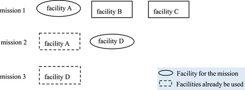
In the scenario illustrated in Figure 6, not all of the missions are served, which means that the problem can be considered complex and the use of the heuristic method is not appropriate. In this case, Steps 2 and 3 are also needed. And ‘complex scenarios’ include 2 situations: (1) when there are sufficient facilities, but the mapping relationship between available facility sets for missions is complex, making it difficult for heuristic algorithms to assign available facilities to each mission; (2) when there are insufficient facilities to serve all the missions. Both situations require the use of decomposition algorithms to obtain better solutions. In contrast, ‘non-complex scenario’ refers to the situation that all the missions can be served by available facilities. For those non-complex problems, the solution obtained using the heuristic method is output as the final result.

3.2.2. Determination of the status of the facilities (Step 2)

The mission time optimization produces many binary variables and constraints. For complex scenarios, this makes it difficult to find a solution to the scheduling problem for a single ground station within an acceptable time. So, the model with fixed mission times can reduce the number of binary variables and make a model of smaller scale. In the discussion below, the mission time is assumed to be constant (it cannot be adjusted and the mission has the same beginning and end times as the visible time range). The status of the facilities is then determined on this basis.

3.2.2.1. Objective

The objective is to minimize the penalty that results from having unserved missions. This includes (1) a penalty for arranging the antenna (which might actually be more appropriate here) (denoted by $C_4$ in Equation (34)), (2) a penalty for the arranged demodulators (denoted by $C_2$ in Equation (2)), and (3) a penalty for the arranged recorders (denoted by $C_5$ in Equation (35)): (36) $min(C_2+C_4+C_5)$(36) (37) $C_4=\sum _{}p{a}_i^1\ast \left(1-\sum _{}an{t}_{ij}\right)+\sum \sum w{a}_{ij}\ast an{t}_{ij},i\in I,j\in J$(37) (38) $C_5=\sum p{r}_i^1\ast \left(1-\sum re{c}_{ik}\right)+\sum \sum w{r}_{ik}\ast re{c}_{ik},i\in I,k\in K$(38)

3.2.2.2. Constraints

As the mission time is fixed, many of the intermediate variables and constraints needed for the time adjustment are unnecessary and the facility switch-time constraints are adjusted as explained below.

Antenna $j$ cannot serve mission $i^{\mathrm{\prime }}$ within time $\tau$ of the end of the previous mission (mission $i$): (39) $b_{i^{\mathrm{\prime }}}\ge c_i+\tau -M(2-an{t}_{ij}-an{t}_{i^{\mathrm{\prime }}j}),\mathrm{\forall }i,i^{\mathrm{\prime }}\in I,i^{\mathrm{\prime }}>i,j\in J_{i{i}^{}.}$(39)

Also, demodulator $g$ cannot serve mission $i^{\mathrm{\prime }}$ within time $\tau$ of the end of the previous mission: (40) $b_{i^{\mathrm{\prime }}}\ge c_i+\tau -M(2-dem{o}_{ig}-dem{o}_{i^{\mathrm{\prime }}g}),\mathrm{\forall }i,i^{\mathrm{\prime }}\in I,i^{\mathrm{\prime }}>i,g\in G$(40)

Finally, recorder $k$ cannot serve mission $i^{\mathrm{\prime }}$ within time $\tau$ of the end of the previous mission: (41) $c_{i^{\mathrm{\prime }}}-p{t}_{i^{\mathrm{\prime }}}\ge C_i+\tau -M(2-re{c}_{ik}-re{c}_{i^{\mathrm{\prime }}k}),\mathrm{\forall }i,i^{\mathrm{\prime }}\in I,i^{\mathrm{\prime }}>i,k\in K$(41) The other constraints are described by Equations (1), (11), (12), (15), (16), and (19)-(22).

3.2.3. Optimization of the mission time (Step 3)

The binary variables describing the status of the facilities that were determined in Step 2 are imported into this step. As a result, the optimization search space is reduced significantly and the model can produce a solution rapidly. This step produces solutions for the continuous variables; that is, the beginning and end times of the missions are optimized, and the final scheduling scheme is obtained.

We call the open-source solver COIN CLP/CBC in which dual simplex method is applied to this problem. The objective of this step is described by Equations (23)-(26) and the constraints by Equations (1)–(21).

4. Case study

In this section, some real cases are described. The proposed algorithm was written in Python 2.7.13, and all the cases were run on the open-source solver COIN CLP/CBC (Pulp 1.6.9) on a Dell PC with a 3.20-GHz Intel Core i5-6500 CPU and an 8.0-GB RAM, operating under Windows 7.

The flowchart shown in Figure 1 also applies to the real cases described here.

4.1. Parameters

The numbers of ground stations and missions involved in the cases that were analyzed are shown in Table 4.

Table 4. The numbers of missions and satellites in the analyzed cases.

Case	Number of ground stations	Number of missions
1	2	61
2	2	90
3	3	115
4	3	143
5	4	177
6	4	232
7	5	259
8	5	281
9	6	324
10	6	346

Details of the ground stations and their facilities, including the numbers of antennas, demodulators, and recorders, are shown in Table 5. ‘for TT&C’ denotes antennas that are available for TT&C missions; ‘for DT’ denotes antennas that are available for DT missions. There are some overlaps among the visible ranges of the stations.

Table 5. Number of facilities for the ground stations.

Ground station	Number of antennas		Number of demodulators	Number of loggers
	for TT&C	for DT
Station A	2	8	48	22
Station B	2	7	44	21
Station C	1	6	32	16
Station D	0	1	2	2
Station E	0	1	2	2
Station F	0	1	2	2

PSO is used in Step 1 of the proposed algorithm. And the PSO parameters are listed in Table 6, which include population size NP, the maximum number of iterations Imax, inertial weight $w$, acceleration coefficients $c_1$ and $c_2$. The values of all the parameters are selected based on the typical values in standard PSO and the guidelines of parameter settings.

Table 6. PSO parameters.

NP	Imax	$w$	$c_1$	$c_2$
40	50	0.8	2	2

4.2. Comparisons

In this section, we conduct a comparison between the proposed decomposition algorithm and the previously used genetic algorithm for scheduling in the RSGS operating system. Due to lack of access to obtaining or modifying the parameters, we can only use the results from the default parameters of the genetic algorithm. To ensure accuracy, each case was independently solved 20 times using both methods on the same computer.

For all the cases, the solution statistics of the proposed method and GA are summarized in Tables 7 and 8. In these tables, columns ‘AVG’, ‘BEST’, ‘WORST’, and ‘SD’ denote the average, best, worst value, and the standard deviation of objective values obtained by both methods, respectively. For the proposed decomposition algorithm, Step 2 and Step 3 were run on the open-source solver COIN CLP/CBC, and the stopping criterion for Step 2 and Step 3 of the optimization was that the optimality gap should be smaller than 0.5%.

Table 7. Objective values for the proposed algorithm and GA.

Case	Approach	AVG	BEST	WORST	SD
1	Proposed algorithm	5.7	5.2	6.2	0.5
	GA	10.2	7.4	12.6	1.2
2	Proposed algorithm	57.0	55.2	58.7	1.3
	GA	207.3	79.4	332.2	73.2
3	Proposed algorithm	13.3	11.8	14.6	0.9
	GA	28	20.9	35.2	4.6
4	Proposed algorithm	225.6	224.7	226.4	0.7
	GA	869.3	517	1237.0	226.5
5	Proposed algorithm	28.6	27.8	29.3	0.5
	GA	32.3	29.7	36.4	2.5
6	Proposed algorithm	410.8	410.0	411.7	0.5
	GA	502.3	445.1	577.3	49.8
7	Proposed algorithm	891.3	885.6	899.7	4.6
	GA	1433.2	1317.7	1583.3	107.5
8	Proposed algorithm	3121.4	3103.3	3142.0	11.4
	GA	4748.3	4181.8	5404.1	382.1
9	Proposed algorithm	68.8	66.9	70.5	1.2
	GA	212.1	120.6	322.0	76.5
10	Proposed algorithm	225.8	220.3	231.9	3.3
	GA	661.8	621.6	694.3	27.9

Table 8. Relative percentage differences of objective values and computational times for the two approaches.

Case	Relative percentage difference of objective values (%)				Average computational time for the proposed algorithm (s)	Computational time for GA (s)	Relative percentage difference of computational times (%)
	AVG	BEST	WORST	SD
1	44.6	29.7	50.8	57.5	6.7	7.7	13.0
2	72.5	30.5	82.3	98.2	7.2	8.1	11.1
3	52.5	43.5	58.5	80.4	11.3	15.1	25.2
4	74.0	56.5	81.7	99.7	14.6	26.8	45.5
5	11.5	6.4	19.5	80.0	17.6	37.1	52.6
6	18.2	7.9	28.7	99.0	18.1	44.5	59.3
7	37.8	32.8	43.2	95.7	22.3	54.1	58.8
8	34.3	25.8	41.9	97.0	21.7	76.7	71.7
9	67.6	44.5	78.1	98.4	24.6	77.1	68.1
10	65.9	64.6	66.6	88.2	25.2	81.4	69.0

Table 8 shows the relative differences between the objective values and the computational times obtained using the decomposition algorithm and the genetic algorithm. The relative difference is calculated by dividing the absolute difference by the genetic algorithm result. And the absolute difference refers to the numerical gap between the two algorithm results, with the decomposition algorithm result being subtracted from the genetic algorithm result.

An important reason for utilizing the proposed algorithm is to reduce computation time. In real-life situations, scheduling needs to be quick, especially in emergency missions. As shown in Table 8, results indicate that the proposed algorithm requires less CPU time than the genetic algorithm, with a reduction ranging from 11.1% to 71.7%. Furthermore, as the scale of the case increases, the proposed method exhibits even greater efficiency improvements compared to the genetic algorithm. For results of the value of objectives, the objective value of the proposed algorithm is much smaller than that of the genetic algorithm in some cases (such as case 2, 4, 9, and 10). The reason is that the total lengths of the served missions optimized by these methods are different in those cases. For case 1, 3and 5, the objective values are smaller as the facilities are sufficient to serve all the missions, and the facilities arranged for the missions by the two methods are different and causes differences in objective values. That is, the proposed algorithm assigns facilities with higher priorities to the missions. The standard deviation of the objective values by the proposed algorithm is small because Step 2 and Step 3 of the proposed algorithm are based on solving MILP models. A detailed analysis of these results is presented in Appendix.

5. Conclusions

In this study, facility scheduling of multiple ground stations and multiple satellites was conducted to make full use of facilities for DT and TT&C satellite missions of RSGS. A continuous time-based MILP model that took into account differences in performance between available facilities, load-balancing between facilities, and the confliction of antennas was developed. In order to meet the requirements of the automated scheduling of facilities, this model described all of the scheduling processes necessary for the management of scheduling in RSGS. As the large-scale model was difficult to solve, a decomposition algorithm was proposed for application to the scheduling problem. The results that were obtained using the proposed algorithm were compared to those obtained by the genetic algorithm previously used for scheduling in the RSGS operating system, and the results demonstrated the effectiveness of the proposed algorithm. It was found that the total served mission time obtained using the proposed algorithm was greater than that obtained using the genetic algorithm. In addition, the required computation time was shorter for the proposed algorithm. The proposed algorithm has been already running online and meets the operational requirements of RSGS.

Nomenclature
$i,i^{\mathrm{\prime }}$	=	Mission
$j$	=	Antenna
$g$	=	Demodulator
$k$	=	Recorder
$p$	=	Particle
$t$	=	the number of iteration for PSO

Set
$I$	=	the set of missions
$J$	=	the set of antennas
$G$	=	the set of demodulators
$K$	=	the set of recorders
$I^{up}$	=	the set of TT&C missions
$P$	=	the set of particles

Variables
$an{t}_{ij}$	=	binary variable, $ant{e}_{ij}=1$ denotes that mission $i$ is served by antenna $j$
$b_i$	=	the beginning time of mission $i$
$c_i$	=	the end time of mission $i$
$or{d}_{i{i}^{\mathrm{\prime }}}$	=	binary variable, $or{d}_{i{i}^{\mathrm{\prime }}}=1$ denotes that the beginning time of mission $i$ is earlier than that of mission $i^{\mathrm{\prime }}$
$ma{t}_i$	=	denotes the length of an incomplete mission $i$
$chan{l}_i$	=	denotes the number of channels used in mission $i$
$dem{o}_{ig}$	=	binary variable, $dem{o}_{ig}=1$ denotes that demodulator $g$ serves mission $i$
$re{c}_{ik}$	=	binary variable, $re{c}_{ik}=1$ denotes that mission $i$ is served by recorder $k$
$z_{ik}$	=	denotes the number of missions using recorder $k$ at the same time as mission $i$
$y_{i{i}^{\mathrm{\prime }}}$	=	binary variable, $y_{i{i}^{\mathrm{\prime }}}=1$ denotes that the time interval between missions $i$ and $i^{\mathrm{\prime }}$ is smaller than the recorder switching time
$p{s}_i$	=	binary variable, $p{s}_i=1$ denotes that mission $i$ is not served
$X_p$	=	the position of a particle $p$
$x_{i,j}$	=	the value of $x_{i,j}$ denotes the probability of antenna j serving mission i, and $0\le x_{i,j}\le 1$.
$Ve{l}_p$	=	the velocity of particle $p$

Parameters
$M$	=	a large positive number, and M = 106 in this paper
$\tau$	=	switching time of facilities
$s{t}_i$	=	the beginning of this visible time range for mission $i$
$t{e}_i$	=	the end of this visible time range for mission $i$
$Grou{p}_i$	=	the group to which mission $i$ belongs
$chan{l}_i$	=	the number of channels of mission $i$
$Inj{a}_i$	=	the missions that overlap with mission $i$
$nu{m}_k$	=	the number of recorder k’s channels
$p{t}_i$	=	the time length of the visible range for mission $i$
$rat{e}_i$	=	the rate of mission $i$
$trat{e}_k$	=	the rate of recorder $k$
$p{a}_i^1$	=	denoting a penalty that results if mission $i$ not served by any antenna
$p{a}_i^2$	=	denotes the penalty of unit incomplete time of mission $i$
$p{c}_i$	=	is a penalty that is assigned if no antenna is arranged for mission $i$
$p{r}_i^1$	=	gives the penalty for mission $i$ not being served by any recorder.
$w{r}_{ik}$	=	the priority given to recorder $k$ serving mission $i$
$w{a}_{ij}$	=	denotes the priority given to antenna $j$ serving mission $i$
$Alin{k}_{jg}$	=	$Alin{k}_{jg}=1$ denotes that antenna $j$ is connectable to facility $g$.
$Rlin{k}_{kg}$	=	$Rlin{k}_{kg}=1$ denotes that recorder $k$ is connectable to facility $g$.
$w$	=	inertial weight
$c_1$	=	acceleration coefficient
$c_2$	=	acceleration coefficient
$pbes{t}_p^t$	=	the best of particle $p$ in iteration $t$
$gbes{t}^t$	=	the best of all the particles in iteration $t$
$T$	=	the maximum number of iterations for PSO

Data deposition

https://doi.org/10.6084/m9.figshare.21729008.

Geolocation information

There’s no geolocation information in the study of this article. And the coordinate of the authors’ institute is: 40.07106°N, 116.28226°E.

Data available statement

The authors confirm that the data supporting the findings of this study are available within the article.

Acknowledgements

The authors wish to thank the reviewers for their constructive comments and suggestions for improving the manuscript.

Disclosure statement

No potential conflict of interest was reported by the author(s).

Additional information

Funding

This work is supported by the Strategic Priority Research Program of the Chinese Academy of Sciences [grant number XDA19010401].

Appendix

In this section, a detailed analysis of an illustrative example is given. The analysis examines the differences between the mission states and mission times produced by the two methods. The example is provided to explain the specific reasons for the variation in objective function values between the two methods.

A1.1. Number of unserved missions and length of missions

Table A1 shows the total lengths of the completely served missions that were obtained using the genetic algorithm and the proposed algorithm. In case 4, there are 143 missions; 142 of these are completely served in the results produced by the proposed algorithm, and 1 mission is partially served. In the results produced by the genetic algorithm, 141 missions are completely served and 2 missions are not served. The value of the ‘unserved rate’ in the table is equal to the ‘total time of unserved missions’ divided by total time of all the missions. Using the proposed algorithm, there was an increase of 435s in the total mission time compared to the genetic algorithm, whereas the unserved rate was reduced by about 2/3.

Table A1. Comparison between number and lengths of completed missions for the genetic algorithm and proposed algorithm.

Approach	Number of completely served missions	Number of partially served missions	Number of unserved missions	Total time length of served missions (s)	Total time length of unserved missions (s)	Unserved rate (%)
Proposed algorithm	142	1	0	79,995	240	0.30
GA	141	0	1	79,560	675	0.85

A1.2. Facility scheduling results

A selection of the facilities scheduling results for case 1 are shown in Table A2. The time period covered by the missions is 0:14:55–1:11:28, and all of the missions served by the same ground station with overlap in time. Each mission is assigned a priority from 1–5 (1 being the highest and 5 the lowest priority).

Table A2. Scheduling results for a selection of the missions from case 1.

Mission	Priority	Satellite	Station	Beginning time	End time
1	1	G-1	Station A	0:14:55	0:19:55
2	5	JL-1	Station A	0:18:01	0:23:19
3	5	CB-1	Station A	0:39:27	0:44:27
4	3	ZY-1	Station A	0:44:51	0:53:06
5	2	G-2	Station A	0:47:10	0:56:50
6	5	JL-2	Station A	0:49:50	0:55:01
7	2	G-3	Station A	0:51:58	1:00:09
8	5	H-1	Station A	0:55:31	1:05:37
9	1	G-4	Station A	1:00:14	1:03:14
10	4	ZY-2	Station A	1:04:42	1:11:28

The facility sets, including antennas, demodulators, and recorders, that are available for these missions are shown in Table A3. The sets differ for each mission because of the differences in performance between facilities.

From Table A3, it can be seen that the number of antennas is adequate relative to that of the recorders and demodulators.

Table A3. Facility sets available for missions.

Mission	Satellite	Available antennas	Available demodulators	Available Recorders
1	G-1	A-3; A-4; A-5	R-D; R-E; R-H; R-I	D-K1;D-K2;D-K3;D-K4;D-L1;D-L2;D-L3;D-L4
2	JL-1	A-3; A-4; A-5	R-F; R-G; R-H; R-I	D-J1;D-J2;D-J3;D-J4;D-J5;D-J6
3	CB-1	A-1; A-2	R-A;R-D; R-E	D-J1;D-J2;D-J3;D-J4;D-J5;D-J6; D-K1;D-K2;D-K3;D-K4;D-L1;D-L2;D-L3;D-L4
4	ZY-1	A-2;A-3; A-4; A-5	R-A;R-D; R-E	D-J1;D-J2;D-J4;D-J5; D-K1;D-K2;D-K3;D-K4;D-L1;D-L2;D-L3;D-L4
5	G-2	A-3; A-4; A-5	R-D; R-E; R-H; R-I	D-K1;D-K2;D-K3;D-K4;D-L1;D-L2;D-L3;D-L4
6	JL-2	A-3; A-4; A-5	R-H; R-I	D-J1;D-J2;D-J3;D-J4;D-J5;D-J6
7	G-3	A-2;A-3; A-4; A-5	R-A;R-D; R-E	D-J1;D-J2;D-J4;D-J5; D-K1;D-K2;D-K3;D-K4;D-L1;D-L2;D-L3;D-L4
8	H-1	A-3; A-4; A-5	R-F; R-G; R-H; R-I	D-J1;D-J2;D-J3;D-J4;D-J5;D-J6; D-L1;D-L2;D-L3;D-L4
9	G-4	A-2;A-3; A-4; A-5	R-A;R-D; R-E	D-J1;D-J2;D-J4;D-J5; D-K1;D-K2;D-K3;D-K4;D-L1;D-L2;D-L3;D-L4
10	ZY-2	A-2;A-3; A-4; A-5	R-A;R-D; R-E	D-J1;D-J2;D-J4;D-J5; D-K1;D-K2;D-K3;D-K4;D-L1;D-L2;D-L3;D-L4

The scheduling results obtained using the genetic algorithm and the proposed algorithm are shown in Tables A4 and A5, respectively.

In the results shown in Table A4, mission 4 and 9 are not served because the number of antennas is insufficient from the optimization results of genetic algorithm. These two missions cannot be served even though there are sufficient demodulators and recorders available. Missions 4 and 9 have lengths of 495 and 180 s, respectively – a total length of 675 s. The arrangements of the antennas, recorders and demodulators are also given in Table A4. The number of demodulators is equal to the number of data channels in each case.

Table A4. Scheduling results obtained using the genetic algorithm.

Mission	Mission be served or not	Beginning time	End time	Antenna	Recorder	demodulator
1	completely served	0:14:55	0:19:55	A-4	R-E	D-G1; D-G2
2	completely served	0:18:01	0:23:19	A-5	R-G	D-J1; D-J2
3	completely served	0:39:27	0:44:27	A-1	R-B	D-E1; D-E2; D-E3; D-E4; D-E5
4	not served	0:44:51	0:53:06	–	–	–
5	completely served	0:47:10	0:56:50	A-3	R-E	D-G1; D-G2
6	completely served	0:49:50	0:55:01	A-5	R-H	D-J3; D-J4
7	completely served	0:51:58	1:00:09	A-2	R-A	D-G3; D-G4
8	completely served	0:55:31	1:05:37	A-4	R-G	D-H1; D-H2
9	not served	1:00:14	1:03:14	–	–	–
10	completely served	1:04:42	1:11:28	A-3	R-D	D-Z1; D-Z2

The scheduling results obtained using the proposed algorithm are shown in Table A5. In this case, mission 6 is partially served, with 240 s of the mission not being served. This mean that the served mission time is 435 s longer than for the genetic algorithm.

Table A5. Scheduling results obtained using the proposed algorithm.

Mission	Mission be served or not	Beginning time	End time	Antenna	Recorder	Demodulator
1	completely served	0:14:55	0:19:55	A-4	R-E	D-G1; D-G2
2	completely served	0:18:01	0:23:19	A-5	R-G	D-J1; D-J2
3	completely served	0:39:27	0:44:27	A-1	R-B	D-E1; D-E2; D-E3; D-E4; D-E5
4	completely served	0:44:51	0:53:06	A-2	R-D	D-Z1; D-Z2
5	completely served	0:47:10	0:56:50	A-4	R-I	D-G1; D-G2
6	partially served	0:49:50	0:51:01	A-5	R-H	D-J3; D-J4
7	completely served	0:51:58	1:00:09	A-3	R-A	D-G3; D-G4
8	completely served	0:55:31	1:05:37	A-5	R-G	D-H1; D-H2
9	completely served	1:00:14	1:03:14	A-2	R-E	D-G1; D-G2
10	completely served	1:04:42	1:11:28	A-3	R-D	D-Z1; D-Z2

References

- An, Y., W. Li, W. Wang, X. Yang, P. Wei, and X. Wang. 2021. “Research on Schedule Strategy of Ground Stations for LEO Satellites.” Journal of Time and Frequency 44 (2): 120–131.
- Falone, R., and G. Corrao. 2018. “Ground Station Network Scheduling Through Genetic and Deterministic Combined Algorithm.” Paper Presented at the 2018 Space Ops Conference, Palais du Pharo, May 28–June 1.
- Fan, H., W. Zhang, M. Tian, G. Ma, and B. Cheng. 2022. “A Resource Scheduling Method for Satellite Mission Ground Station Based on Particle Swarm Optimization Algorithm.” Journal of University of Chinese Academy of Sciences 39 (6): 801–808. https://doi.org/10.7523/j.ucas.2021.0012.
- Goldberg, D. E. 1989. Genetic Algorithms in Search, Optimization, and Machine Learning. Boston, MA: Addison-Wesley.
- Harjunkoski, I., C. T. Maravelias, P. Bongers, P. M. Castro, S. Engell, I. E. Grossmann, J. Hooker, C. Mendez, G. Sand, and J. Wassick. 2014. “Scope for Industrial Applications of Production Scheduling Models and Solution Methods.” Computers & Chemical Engineering 62:161–193. https://doi.org/10.1016/j.compchemeng.2013.12.001.
- Iacopino, C., P. Palmer, N. Policella, and A. Donati. 2014. “Planning the GENSO Ground Station Network via an Ant Colony-Based Approach.” Paper Presented at the 13th International Conference on Space Operations, Pasadena, CA, May 2014. https://doi.org/10.2514/6.2014-1704.
- Kennedy, J. 2005. “Why Does It Need Velocity?” Paper Presented at Proceedings of the IEEE Swarm Intelligence Symposium (SIS’05), Pasadena, CA, June 8–10.
- Kennedy, J., and R. Eberhart. 1995. “Particle Swarm Optimization.” Paper Presented at Proceedings of the IEEE International Conference on Neural Networks, Perth, November 27–December 1. https://doi.org/10.1109/ICNN.1995.487241.
- Ko, H. P. 2016. “Discretized Genetic Algorithm for Satellite Constellation and Multiple Ground Antenna Scheduling.” Paper Presented at the 14th International Conference on Space Operations, Daejeon, May 16–20.
- Li, X., X. Guo, H. Tang, R. Wu, and J. Liu. 2023. “An Improved Cuckoo Search Algorithm for the Hybrid Flow-Shop Scheduling Problem in Sand Casting Enterprises Considering Batch Processing.” Computers & Industrial Engineering 176. https://doi.org/10.1016/j.cie.2022.108921.
- Li, Y., R. Wang, Y. Liu, and M. Xu. 2015. “Satellite Range Scheduling with the Priority Constraint: An Improved Genetic Algorithm Using a Station ID Encoding Method.” Chinese Journal of Aeronautics 28 (3): 789–803. https://doi.org/10.1016/j.cja.2015.04.012 .
- Li, J., T. Zhang, and G. Ye. 2015. “Satellite-Ground TT&C United Scheduling Methods of GNSS Constellation Based on Nodes Constraint.” In Vol.1 of China Satellite Navigation Conference (CSNC) 2015 Proceedings, 55–66. Heidelberg: Springer .
- Lin, W. C., C. Y. Liu, D. Y. Liao, and Y. Y. Lee. 2003. “Daily Imaging Scheduling of an Earth Observation Satellite.” Poster Presented at the 2003 IEEE International Conference on Systems, Man and Cybernetics. Washington, DC, October 5–8.
- Marinelli, F., S. Nocella, F. Rossi, and S. Smriglio. 2011. “A Lagrangian Heuristic for Satellite Range Scheduling with Resource Constraints.” Computers & Operations Research 38 (11): 1572–1583. https://doi.org/10.1016/j.cor.2011.01.016.
- Petelin, G., M. Antoniou, and G. Papa. 2021. “Multi-Objective Approaches to Ground Station Scheduling for Optimization of Communication with Satellites.” Optimization and Engineering. https://doi.org/10.1007/s11081-021-09617-z.
- Shang, X., Y. Feng, J. Chen, W. Zhang, P. Huang, Q. Kong, L. Han, et al. 2014. Ground receiving resource allocation method based on receiving resource capability constraints. China Patent CN201410310281.0, filed October, 22.
- Song, Y., B. Song, L. Xing, Y. Jia, and Y. Chen. 2022. “Improved Artificial Bee Colony Algorithm for Satellite-Ground Cooperative Observation Planning Problem.” Control and Decision 37 (3): 555–564. https://doi.org/10.13195/j.kzyjc.2020.1459.
- Spangelo, S., J. Cutler, K. Gilson, and A. Cohn. 2015. “Optimization-Based Scheduling for the Single-Satellite, Multi-Ground Station Communication Problem.” Computers & Operations Research 57:1–16. https://doi.org/10.1016/j.cor.2014.11.004.
- Sun, J., and F. Xhafa. 2011. “A Genetic Algorithm for Ground Station Scheduling.” Paper Presented at International Conference on Complex, Intelligent and Software Intensive Systems, Seoul, June 30–July 2.
- Tian, M., S. Xu, P. Huang, G. Ma, and K. Feng. 2020. “Intelligent Scheduling Method for Satellite Ground Station Resources.” In Proceedings of the 39th Chinese Control Conference, 392–397. Shenyang: IEEE.
- Wang, Z., Z. Zhang, and Y. Chen. 2019. “Multi-Objective Optimization of Satellite-Ground Time Synchronization Scheduling Problem.” In Proceedings of the 2019 IEEE Congress on Evolutionary Computation (CEC), 530–537. Wellington: IEEE.
- Xhafa, F., and W. H. Andrew. 2021. “Optimisation Problems and Resolution Methods in Satellite Scheduling and Space-Craft Operation: A Survey.” Enterprise Information Systems 15 (8): 1022–1045. https://doi.org/10.1080/17517575.2019.1593508.
- Xhafa, F., A. Barolli, and M. Takizawa. 2013. “Steady State Genetic Algorithm for Ground Station Scheduling Problem.” Paper Presented at 2013 IEEE 27th International Conference on Advanced Information Networking and Applications, Barcelona, March 25–28 .
- Xhafa, F., X. Herrero, A. Barolli, L. Barolli, and M. Takizawa. 2013. “Evaluation of Struggle Strategy in Genetic Algorithms for Ground Stations Scheduling Problem.” Journal of Computer and System Sciences 79 (7): 1086–1100. https://doi.org/10.1016/J.JCSS.2013.01.023 .
- Xhafa, F., J. Sun, A. Barolli, M. Takizawa, and K. Uchida. 2012. “Evaluation of Genetic Algorithms for Single Ground Station Scheduling Problem.” In 2012 IEEE 26th International Conference on Advanced Information Networking and Applications, 299–306. Fukuoka: IEEE.
- Xu, Y., X. Liu, R. He, and Y. Chen. 2020. “Multi-Satellite Scheduling Framework and Algorithm for Very Large Area Observation.” Acta Astronautica 167:93–107. https://doi.org/10.1016/j.actaastro.2019.10.041.
- Yan, Y., P. Castro, Q. Liao, and Y. Liang. 2021. “An Effective Decomposition Algorithm for Scheduling Branched Multiproduct Pipelines.” Computers & Chemical Engineering 154. https://doi.org/10.1016/j.compchemeng.2021.107494.
- Zhang, Z., Y. Chen, L. He, L. Xing, and Y. Tan. 2019. “Learning-Driven Many-Objective Evolutionary Algorithms for Satellite-Ground Time Synchronization Task Planning Problem.” Swarm and Evolutionary Computation 47:72–79. https://doi.org/10.1016/j.swevo.2017.05.011.
- Zhang, Z., Y. Jiang, X. Gao, and D. Huang. 2016. “An Efficient Two-Level Hybrid Algorithm for the Refinery Production Scheduling Problem Involving Operational Transitions.” Industrial & Engineering Chemistry Research 55 (28): 7768–7781. https://doi.org/10.1021/acs.iecr.6b00631.