Modification of a linear regression-based multi-model super-ensemble technique and its application in forecasting of wave height during extreme weather conditions

ABSTRACT

In this study, we focus on the improvement of wave forecast of the Indian coastal region using a multi-model ensemble technique. Generally, a number of wave forecast are available for the same region from different wave models. The main objective of this study is to merge the wave forecasts available at Indian National Centre for Ocean Information Services from different wave models to obtain an improved wave forecast using a multi-model super-ensemble method [Krishnamurti et al. 1999. Improved weather and seasonal climate forecasts from multi-model super-ensemble. Science. 285:1548–1550] during extreme weather conditions and to modify Krishnamurthy’s techniques and validate with observations for a better prediction. Here, Multi-grid WAVEWATCH III, Simulating WAves Nearshore and MIKE 21 Spectral Waves are used for the generation of wave forecast. We propose a modification of Krishnamurthy’s linear regression-based ensemble model. By using both of these ensemble techniques, we perform a multi-model ensemble forecasting of significant wave height up to 24-h lead time in the Indian Ocean for three different cyclones (Nilofar, Hudhud and Phailin) and during the southwest monsoon. A comparison of ensemble predictions and individual model predictions with the actual observations showed generally satisfactory performance of the chosen tools. At the time of severe cyclones such as Hudhud and Phailin, our modified technique shows significantly better prediction than the linear regression-based ensemble technique.

1. Introduction

Progressive improvement in wave modelling now enables the generation of accurate wave forecast even during the extreme weather conditions. This improvement is achieved through research in the last decades which has led to the development of many third-generation global and regional wave models such as WAVEWATCH III (WWIII), Simulating WAves Nearshore (SWAN) and MIKE 21 Spectral Waves (SW). The accurate wave information is essential for marine activities, offshore and coastal constructions, shipping and coastal population especially during the extreme weather conditions. Operational forecasting agencies make use of the available wave models for the forecast generation in a regional and global scale. Several wave forecasts are available for a region from different wave models. The selection of the best forecast is a difficult task for the forecaster since the model performance would never be consistent for a region. This inconsistency can be because of the forcing of model physics. The decision-making would be crucial especially during the extreme weather conditions. An ensemble technique can merge different forecasts to a better wave forecast compared to the individual model forecasts.

The ensemble technique deals with the uncertainties in a forecast to improve it. The uncertainties in the forecast can be caused by the initial conditions, numerical techniques, parameterisation schemes and nonlinearity of a natural system. Therefore, scientists invoked the idea of ensemble forecasting (Lorenz 1965, Leith 1974, Toth and Kalnay 1993). Multiple model outputs are used for ensemble and the ensemble prediction should be less erroneous compared to individual outputs. Krishnamurti, Kishtawal, Zhang et al. (2000) proposed a linear regression-based multi-model super-ensemble forecasting method, which is an effective post-processing technique in reducing model output errors. Krishnamurti, Kishtawal, Shin et al. (2000) showed the efficiency of ensemble technique to improve weather and seasonal climate forecasts. The super-ensemble technique was applied for forecasting tropical precipitation (Krishnamurti, Kishtawal, Zhang et al. 2000; Krishnamurti et al. 2007; Chakraborty and Krishnamurti 2009) and tracking of tropical cyclones in the Pacific (Kumar et al. 2003). Recently, this method has been further explored with dynamical linear models, from the Kalman Filter (Shin and Krishnamurti 2003a) to probabilistic approaches (Shin and Krishnamurti 2003b). In oceanography, the use of multi-model statistics has been shown to improve the prediction of temperature (Logutov and Robinson 2005, Rixen et al. 2009) and acoustic properties (Rixen and Coelho 2006) in the water column. By combining models of different nature, the concept of hyper-ensemble is introduced to improve surface drift predictions (Rixen and Coelho 2007; Vandenbulcke et al. 2009). More recently, Lenartz et al. (2010) have applied the super-ensemble technique to wave forecast during normal weather conditions.

In the present study, we focus on the improvement of wave forecast for the Indian coastal region during the extreme weather conditions such as cyclones using a multi-model ensemble technique. In the North Indian Ocean, cyclones are common in the post-monsoon season (October–December). The dissemination of accurate ocean state/wave forecast during cyclones is always a challenging task for the operational agencies. Earth System Science Organization-Indian National Centre for Ocean Information Services (ESSO-INCOIS), which is the only national agency in India for issuing ocean state forecast, uses three different wave models, namely Multi-grid WWIII, SWAN and MIKE 21 SW for the generation of wave forecast. The main objective of this study is

1. To modify Krishnamurthy’s super-ensemble technique (Krishnamurti, Kishtawal, Zhang et al. 2000).

2. To merge the wave forecasts available at INCOIS from different wave models to obtain an improved wave forecast using this modified multi-model super-ensemble method for the extreme weather conditions.

For the study, three severe cyclones, Phailin (October 2013), Hudhud (October 2014) and Nilofar (October 2014), are selected.

2. Severe cyclones Phailin, Hudhud and Nilofar

Phailin developed from a cyclonic circulation of the South China Sea. The cyclonic circulation lay as a low-pressure are over the Tenasserim coast on 6 October 2013. It concentrated into a depression over the same region on 8 October near latitude 12°N and longitude 96°E. Moving west–northwestwards, it intensified into a deep depression on 9th morning and further into a cyclonic storm (CS), ‘Phailin’ in the evening of the same day. Moving northwestwards, it further intensified into a severe cyclonic storm (SCS) in the morning and into a very SCS in the forenoon of 10th October over east central Bay of Bengal (BOB) (Figure 1). Phailin crossed Odisha and adjoining north Andhra Pradesh coast near Gopalpur around 22:30 h IST of 12 October 2013 with a sustained maximum surface wind speed of 200–210 km/h gusting to 220 km/h (Indian Meteorological Department report, October 2013).

Figure 1. Tracks of cyclones Phailin (red), Hudhud (magenta) and Nilofar (green). The positions at 00UTC are marked along the track. The locations of buoys at Gopalpur, Visakhapatnam (VSK), Pondicherry and AD06 are marked in blue.

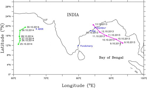
Hudhud (7–14 October 2014) originated from a low-pressure area which was in the Tenasserim coast and adjoining the North Andaman Sea in the morning of 6 October 2014. It intensified into a CS in the morning of 8th October, and crossed the Andaman Islands close to Long Island between 08:30 and 09:30 h IST of 8th October. It then emerged into Southeast BOB and continued to move west–northwestwards. It intensified into an SCS in the morning of 9th October, and further into a very SCS in the afternoon of 10th October. It reached maximum intensity in the early morning of 12th with a maximum sustained wind speed of 180 km/h over the west-central BOB off Andhra Pradesh coast. It crossed north Andhra Pradesh coast over Visakhapatnam between 12:00 and 13:00 h IST of 12th October with the same wind speed. After landfall, it continued to move northwestwards and weakened gradually into SCS in the evening and further into a CS in the same midnight. Then it weakened into a depression in the evening of 13th (Indian Meteorological Department report, October 2014).

Nilofar originated from a low-pressure area which was in the southeast Arabian Sea (AS) in the morning of 21 October 2014. It concentrated into a depression in the early morning of 25th over west-central and adjoining southwest AS. It intensified into a CS over the same region in the morning of 26th. It then moved nearly northwards and further intensified into an SCS over west-central AS in the early morning of 27th and into a very SCS around noon of the same day (Figure 1). It reached its maximum intensity around midnight of 28th with wind speed of 205 km/h. It then moved north–northeastwards and started to weaken rapidly under the influence of high vertical wind shear, entrainment of dry and cold air from the north and relatively lower ocean thermal energy. It weakened into an SCS during early hours of 30th October and into a CS in the afternoon of 30th October. It weakened into a deep depression in the early hours and into a depression in the early morning of 31st October. It weakened into a well-marked low-pressure area over northeast AS off north Gujarat coast in the forenoon of 31st October (Indian Meteorological Department report, November 2014). Figure 1 shows the track of the cyclone.

3. Methodology

In Krishnamurthy’s super-ensemble technique, several model outputs are regressed against the observed data. This technique consists of two stages: training and forecasting periods. In the training period, the weights of the models are determined from the regression coefficients. These evaluated weights are used in the forecasting period. In this period no additional observation is considered. Forecasting is performed based on the weights of the training period and the model outputs of the forecasting period. This method is carried out at each location, i.e. at each grid point separately.

Mathematically, at a given grid point, for a certain forecast time j, the super-ensemble forecasting model is(1)

where S_j represents the real-time super-ensemble value, Ō is the mean observed value during the training period, F_i,j is the forecast value of the ith model at the jth time step, is the mean of the ith model forecast value during the training period and m is the number of the models. Given a set of model outputs F_i, a multiple regression technique is used in which the model outputs are regressed against the observed data in the training period. Then least square minimisation between the super-ensemble output S_j and the observed value O_j is done for deriving the weights a_i. The super-ensemble forecasting value of the forecasting period is computed from Equation (1) by using these values of a_i and the model outputs F_i of the forecasting period, where i varies from 1 to m. Hereafter, Krishnamurthy’s model would be referred as KEM in this text.

Here, a modification of KEM is proposed for improving the ensemble forecasting. This modified ensemble method is denoted as MEM. MEM consists of two steps. In step 1, singular value decomposition (SVD) is performed on the predictor variables F_i. SVD is a robust, algebraic procedure, which transforms the model outputs F_i into an orthogonal mode, say, U1 = (u₁,u₂, … ,u_T). In KEM, model outputs F_i are directly used for regression. In MEM, U1 is used as the predictor variable instead of several F_i. In step 2, we create the three-dimensional time delay vector, say, ((u₁,u₂,u₃), (u₂,u₃,u₄), … ,(u_T-2,u_T-1,u_T)) from U1. Dimension of the time delay vector is chosen empirically as 3. This time delay vector is regressed against the observed data O in the training period. The regression coefficients are used in the forecasting period for generating ensemble prediction. The significance of SVD is that it transforms model outputs into an orthogonal mode U1, which omits the redundant information and represents the key information, contained in the model outputs. This strengthens the predictor variables of MEM compared to KEM. In KEM, at any time step (say, j), observation o_j is regressed by the model outputs at the single time step j. In MEM, at any time step j, o_j is regressed by the time delay vector (u_j-2 ,u_j-1 ,u_j). So we consider several time steps before u_j for regressing the transformed model output U1 against the observation o_j. Here, j varies between 3 to T. This makes MEM more powerful than KEM. These two steps are detailed below.

Step 1. A matrix F is created out of the model outputs, where the ith column of F is the ith model output F_i. Hence, an element of the ith row and the jth column of F matrix Fi,j is the forecast value of the ith model at the jth time. Let us assume that total T time steps are considered in the training period. So F matrix can be formulated asSVD is performed on F to decompose it as UWV^t, where U has T number of rows and T number of columns, W has T number of rows and m number of columns and V is a square matrix of order m. In W matrix, only the m diagonal values are nonzero, everything else is zero. So W can be considered as an m dimensional square matrix and the column number of U ultimately reduces to m, when it is multiplied by W. U is the matrix of the eigenvectors of FF^t and V is the matrix of the eigenvectors of F^t F. Diagonal elements of W are the singular values of F. The idea behind SVD is that most of the variance (power) is contained within the first few columns of U matrix. Diagonal elements of W matrix, say, {w₁ ,w₂ , … ,w_m} are arranged in a decreasing order, i.e. w₁≥w₂≥ w₃ … ≥ w_m. It is assumed that the diagonal elements with a lower magnitude are associated with the noise of the signal. Hence, we omit the negligible singular values and consider the first few significant values, say, {w₁, w₂, w₃, … ,w_d}, where d is less than m. Now, we assign 0 to the (d + 1)th to the mth diagonal elements and this new matrix is denoted as W′. The signal is reconstructed by the relationship F′ = UW′Vt. This reconstructed signal is supposed to contain the key information of matrix F (Broomhead and King 1986, Casdagli et al. 1991). For our experimental data, empirically it is found that all of the diagonal values of W matrix are negligible except the first one. Hence, only the first column of U matrix, say U1, is considered.

Step 2. U1 is now used as the predictor variable, whereas the observed data O is the predictand variable. Abarbanel et al. (1994) have shown that the time delay embedding method can be applied for predicting one variable, say, z = (z₁,z₂,z₃, … ,z_T) from the other variable, say, x = (x₁,x₂,x₃, … ,x_T), where T is the length of z and x. In this method, the time delay vector, say, ((x₁,x₂,x₃), (x₂,x₃,x₄), … ,(x_T-2,x_T-1,x_T)) is created from the time series x. The length of the time delay vector is determined empirically. Here, without loss of generality, it is assumed to be 3. Then a linear or non-linear relationship is established between these time delay vectors of x and z. In the context of ensemble prediction, observation O has to be predicted from U1. Hence, three-dimensional time delay vectors, say, ((u₁,u₂,u₃), (u₂,u₃,u₄), … ,(u_T-2,u_T-1,u_T)) are created from U1in the training period. Here, the multiple linear regression technique is used to fit the time delay vectors to the observed value O. The matrix equation is the following:(2) For finding the coefficients a₁, a₂ and a₃, multiple linear regression is used in the training period. Then the same a_i’s (i = 1,2,3) are used in the forecasting period for generating ensemble prediction.

4. Data used and model description

INCOIS has developed a network of wave rider buoys (WRB) in the Indian coastal water to measure the wave parameters in shallow waters. WRBs are the instruments which float on water surface and have in-built sensors to measure water movements, which in-turn could be converted to wave parameters such as wave heights and wave periods. Significant wave height and wave period from three WRB are used in this study for validation in the coastal areas (Visakhapatnam, Gopalpur and Pondicherry). The data from the moored buoy AD06 deployed in deep water of the AS by the ESSO-National Institute of Ocean Technology (NIOT) are also used for validation. The locations of the buoys are marked in Figure 1. AD06 is in the AS and the other sites are in the coast of the Indian Ocean. The forecast wave data used in this paper comprise three different sources – SW, WWIII and SWAN wave models.

SW is a state-of-the-art third-generation spectral wind wave model developed by Danish Hydraulic Institute (DHI). This model simulates the growth, decay and transformation of wind-generated waves and swells in offshore and coastal areas. SW model is based on flexible mesh and is therefore suitable for both regional and local scale wave modelling, allowing for fine resolution mesh in the shallow regions and coarse resolution mesh in the offshore regions. The model simulates wave growth by the action of wind, non-linear wave–wave interactions, dissipation due to white-capping, bottom friction and depth-induced wave breaking, refraction and shoaling due to depth variations, wave–current interaction and effect of time-varying water depth. Description of all source functions and the numerical methods used in the model are elaborated in Sorensen et al. (2004).

Three different implementations of SW are used in this study. The first one (hereafter SW1) uses the default parameters available with model distribution. This implementation is used to give out operational weather forecasts during normal weather conditions. The second one (hereafter SW2) is specially calibrated for cyclonic conditions by tuning some calibration parameters. Both these implementations use the European Centre for Medium Range Weather Forecasts (ECMWF) winds for forcing the wave models. In the third (hereafter SW3) implementation, we have used the SW model with default parameters, forced with corrected ECMWF winds (corrected spatially using wind observations and wind forecast from India Meteorological Department (IMD)).

Modelled wave fields for the study are generated using WWIII, version 3.14 (Tolman 2014) using the parameterisation scheme ST2 by Tolman and Chalikov (1996). Simulations were performed using a four-grid mosaic. The grids are generated using the bathymetry data ETOPO2 obtained from National Geophysical Data Centre. We have used a spectral grid consisting of 29 frequencies (initial frequency is 0.035 Hz with an increment factor 1.1) and 36 directions. WWIII model could be run as a mosaic of grids with two-way exchange of information between overlapping grids. Each grid is considered as a separate wave model and two-way interaction between all grids is considered continuously transforming the mosaic of individual grids into a single model. The National Centre for Medium Range Weather Forecasting (NCMRWF) forecast winds with 0.25°; 6-hourly resolutions are used for generation of the wave forecast.

SWAN is a state-of-the-art third-generation coastal wave model used for routine wave predictions and can be nested in WWIII. The SWAN validation data off Pondicherry were taken from the operational forecasts of the model running at INCOIS. This model which is nested in WWIII has a uniform spatial resolution of 250 m and gives out 3-hourly forecasts. More details about this model set-up are described in Sandhya et al. (2014). In all of the simulations, the spectral resolutions, physics, numeric, etc. used were identical with those mentioned in Sandhya et al. (2014). The forcing used in SWAN simulations for Nilofar, Hudhud and Phailin was the 3-hourly operational forecasts at 0.25° resolution given out by the ECMWF. Details of the set-up of the wave models (SW, WWIII and SWAN) are given in Table 1.

Table 1. Description of different wave models.

Model	Domain of study	Wind	Resolution
SW1	Indian Ocean, 30°–120° E, −60°–30° N	ECMWF	30°–120°E, 60°S–0° (resolution 110 km), AS and BOB offshore (resolution 45 km), coastal area (resolution 8–15 km)
SW2	Indian Ocean, 30°–120° E, −60°–30° N	ECMWF	Same as SW1
SW3	Indian Ocean, 30°-120° E, −60°–30° N	Corrected ECMWF wind (spatially using wind observations and wind forecast from India Meteorological Department (IMD))	Same as SW1
WWIII	Global, 0°–359° E, −80°–70° N	NCMRWF	Indian Ocean (24°–125° E, −60°–32° N, 50 km), AS (42°–79° E, −5°–31° N, 25 km), BOB (75°–100° E, −5°–23° N, 25 km), coastal grids (East coast(76°–95° E, 5°–23° N, 5 km) and West coast (65°–79° E, 5°–24° N, 5 km)
SWAN	Pondicherry,79.5°–80.5°E, 11.2°–12.2°N AS 60°–79°E, 5°–26°N BOB 76°–95°E, 5°–25°N	ECMWF	250 m
			12 km
			12 km

Apart from wave parameters, results are validated for sea surface temperature (SST) data to establish the significance of this MEM. Monthly mean SST data are taken from Hadley Centre, which is available at http://www.metoffice.gov.uk/hadobs/hadisst/. The Hadley centre SST data are obtained from the Met Office Marine Data Bank (MDB), which also includes data received through the global telecommunications system. Model outputs are taken from a state-of-the-art coupled ocean-atmosphere model, the Climate Forecast System (CFS) (version 2.0). CFS output is downloaded from the website https://nomads.ncdc.noaa.gov/data/cfsr-rfl-mmts/oceansst/.

5. Results and discussions

First ensemble techniques are validated for SST data. Observed SST data are taken at 60°E 10°S location from the Hadley centre website. Six CFS models forecasting M01, M05, M09, M14 and M17 are considered at the same location. Model predictions are performed for the month of March, April and May with January as the initial condition (IC) from 1982 to 2009. Different forecasting is gained from CFS by taking different date and time of January as the IC. Every CFS output consists of 28 data points for each of the 3 sets of predictions. For example, for M01, there are 28 data points for the prediction of March. The first 18 points are taken as the training period and the last 10 points are taken as the forecasting period. Ensemble forecasting is done for the three cases separately. Standard deviation of the observed data is 0.51. RMSE is calculated between observed data and the ensemble members and outputs. RMSE of MEM, KEM, M01, M05, M09, M14, M17 and M21 are 0.4, 0.44, 0.65, 0.73, 0.9, 0.62, 0.51 and 0.94, respectively, for the prediction of March. RMSE of MEM, KEM, M01, M05, M09, M14, M17 and M21 are 0.28, 0.4, 0.36, 0.5, 0.63, 0.42, 0.43 and 0.52, respectively, for April. RMSE of MEM, KEM, M01, M05, M09, M14, M17 and M21 are 0.32, 0.4, 0.48, 0.83, 0.51, 0.54, 0.64 and 0.9, respectively, for May (Table 2). In all of the cases, MEM shows better forecasting than KEM and individual ensemble members.

Table 2. RMSE (in °C) between observation and ensemble members and model predictions of SST for March, April and May with January initial condition.

Period of Prediction	Different models and ensemble techniques	RMSE
Prediction for March (1982–2009)	MEM	0.4
	KEM	0.44
	M01	0.65
	M05	0.73
	M09	0.9
	M14	0.62
	M17	0.51
	M21	0.94
Prediction for April (1982–2009)	MEM	0.28
	KEM	0.4
	M01	0.36
	M05	0.5
	M09	0.63
	M14	0.42
	M17	0.43
	M21	0.53
Prediction for May (1982–2009)	MEM	0.32
	KEM	0.4
	M01	0.48
	M05	0.83
	M09	0.51
	M14	0.54
	M17	0.64
	M21	0.9

Next, this analysis is done for the wave parameters. The analysis is done for the wave period and significant wave height during the southwest monsoon (SWM) (June–August) of 2014 for Pondicherry location. For significant wave height, this analysis is done for three extreme events. In each of these cases, the training period is empirically selected as 2 days and 4 days for significant wave height and wave period, respectively. In the entire cases, ensemble forecasts are generated for the next 24 h. All of the model outputs are 3-hourly data of significant wave height or wave period and hence 8 data points are available for a single day at 00:00 UTC, 03:00 UTC, 06:00 UTC, 09:00 UTC, 12:00 UTC ,15:00 UTC, 18:00 UTC and 21:00 UTC. Total five model outputs are available from SW1, SW2, SW3, SWAN and WWIII. Under normal weather conditions, only three model outputs are used – SWAN, WWIII and SW1 as the other two implementations of SW model are suitable only during cyclones. During cyclones all of the model outputs are used for ensemble. The training period is in the less extreme conditions than the forecast period during cyclones. On the initial one or two days of a cyclone, SW2 and SW3 are not included in the training period, as the training period is in the normal condition on those days. In SW2 implementation, the dissipation at higher frequencies is reduced to obtain the high waves produced by the cyclone. This tuning results in an overestimation of wave heights in the normal monsoon conditions. SW3 implementation uses a bias-corrected wind that is not required for the normal conditions. During the normal condition, ECMWF winds are found to be in good agreement with observations. Even if the winds were accurate for extreme conditions, there is the problem of wind wave generation due to high winds. Hence, the ensemble approach is unavoidable during cyclones.

Although SWAN is nested in WWIII, coastal areas being shallow regions, the effect of boundary conditions is less significant and local sea wind plays a major role there. The AS and the BOB grids used in the cyclone simulations are quite large and so the effect of boundary conditions from WWIII will fade out once the waves travel over large distances from the boundaries. Moreover, the shallow water physics and numeric used in SWAN make it different from WWIII. That is how the SWAN results are different than WWIII results, even if boundary conditions from WWIII are taken. Hence, SWAN and WWIII model results are statistically independent.

At Pondicherry location, results are validated from 19 June to 25 June and from 2 July to 24 July 2014 for the wave period data. Standard deviation of these data is 2.33 second. Figure 2 shows that the RMSEs of wave period for MEM, KEM, SW1, SWAN and WWIII are 2.1, 2.4, 2.7, 2.7 and 3.7, respectively. For a significant wave height, Scatter Index (SI) is also computed. SI is defined as the ratio between RMSE and mean of the observations. During the SWM period of 2014 at Pondicherry location, the study period of significant wave height data is from 1 June 2014 to 28 July 2014 and from 8 August 2014 to 12 August 2014. Table 3 shows that SWAN has a lesser error (RMSE = 0.19, SI = 0.28) compared to the individual models. RMSE for WWIII and SW1 are 0.26 and 0.2, respectively. SI for WWIII and SW1 are 0.38 and 0.3, respectively. For KEM, RMSE is 0.15 and SI is 0.22, whereas for MEM RMSE is 0.12 and SI is 0.17. Thus MEM shows 11%, 21% and 12% lesser error compared to SWAN, WWIII and SW1, respectively. Here, the error percentage is defined as SI multiplied by 100. So, when there is no cyclone, MEM shows 5% less error than KEM.

Figure 2. RMSE (in second) of ensemble and individual model predictions of wave period during SWM of 2014 at Pondicherry.

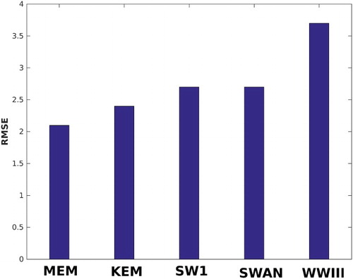
Table 3. RMSE (in metre) and Scatter Index of ensemble and individual model predictions of significant wave height during the southwest monsoon of 2014 and during Nilofar, Hudhud and Phailin cyclones.

Period of prediction	Different models and ensemble techniques	RMSE	Scatter Index
Nilofar (AD06)	MEM	0.26	0.11
	KEM	0.3	0.12
	SWAN	0.31	0.13
	WWIII	0.75	0.3
	SW1	0.63	0.26
	SW2	0.37	0.14
	SW3	0.43	0.17
Hudhud (Vizag)	MEM	0.57	0.17
	KEM	0.91	0.28
	SWAN	1.73	0.54
	WWIII	2.2	0.68
	SW1	0.95	0.3
	SW2	0.78	0.24
	SW3	0.62	0.2
Phailin (Gopalpur)	MEM	0.6	0.21
	KEM	0.72	0.25
	SWAN	0.75	0.26
	WWIII	1.23	0.43
	SW1	0.85	0.3
	SW2	0.9	0.32
SW monsoon (2014) (Pondicherry)	MEM	0.12	0.17
	KEM	0.15	0.22
	SWAN	0.19	0.28
	WWIII	0.26	0.38
	SW1	0.2	0.3

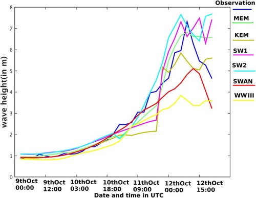
Further, we examine the forecasting performance of ensemble prediction during three severe cyclones, Nilofar, Hudhud and Phailin (Table 3). For Nilofar cyclone we consider the location at AD06 and time period from 26 October 18:00 UTC to 29 October 21:00 UTC. Both SWAN and SW2 models show lesser error than the other individual outputs. Error percentage is 13% and 14% for SWAN and SW2 models, respectively. Compared to SWAN, KEM reduces the error by 1%, whereas for MEM the reduction in error percentage is 3%. Next, the ensemble methods are experimented for Hudhud cyclone at Visakhapatnam from 10 October 00:00 UTC to 12 October 09:00 UTC. SW2 and SW3 wave models show lesser error (24% and 20%, respectively) than the others. For this cyclone, KEM does not give satisfactory prediction. It shows 28% error which is greater than the above two individual models. Our modified version MEM shows only 17% error, which is 3% lesser than the best individual model output. Phailin is studied at the Gopalpur location from 9 October 00:00 UTC to 12 October 21:00 UTC. In this case, the SWAN model shows better result compared to the other individual model outputs. Twenty-six per cent error percentage is shown by SWAN. KEM shows 25% error and MEM shows 21% error. So MEM shows 5% less error than the best model output. For Hudhud, if the SWAN output is not considered MEM shows 20% error, whereas if SW3 is not considered, MEM error grows up to 35% error. For Phailin, if SW2 is not considered, MEM shows 22% error, whereas if SWAN is not considered, the error of MEM grows up to 29%.

Figures 3–5 show the significant wave height for different model outputs, ensemble predictions and the observation. Figure 4 (red circle) indicates that the highest peak is captured by MEM at the exact time with exact accuracy. For Phailin, if we compare the ensemble predictions in Figure 5, we see that MEM captures the highest peak, but KEM cannot capture it. We can conclude that the performance of MEM is significantly better than KEM during severe cyclones like Hudhud and Phailin. If we notice the time series plots of significant wave height for both of these cyclones, we see that each of these has a high peak. Initially KEM performs well, but when a high peak comes in the data, KEM cannot capture it. KEM is based on a linear regression-based technique. In this case, linear regression cannot forecast the wave height if there is sudden change in the time series. It may be because the system becomes so much non-linear that time that linear regression does not work. In our modified approach (MEM), we performed an SVD-based filtering to the predictor variables. We use this filtered output as the predictor variable. This type of filtering does lot of noise reduction and the information about frequency is also accurately contained in this filtered output. That is why MEM has a better forecasting performance than KEM.

Figure 3. Significant wave height (in metre) is plotted for different model outputs, observation and ensemble predictions at the time of Nilofar.

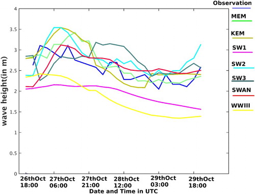
Figure 4. Significant wave height (in metre) is plotted for different model outputs, observation and ensemble predictions at the time of Hudhud.

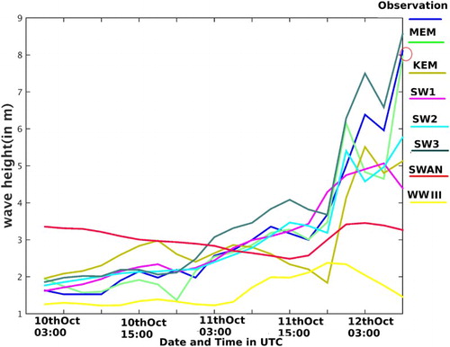
Figure 5. Significant wave height (in metre) is plotted for different model outputs, observation and ensemble predictions at the time of Phailin.

6. Conclusions

In this study, a modification is made to the conventional linear regression-based multi-model super-ensemble method (KEM). For proving the soundness of this modified method (MEM), initially this method is applied to SST data. MEM shows better result than KEM for these data. By using both of these ensemble techniques, we perform a multi-model ensemble forecasting of significant wave height and wave period up to 24-h lead time in the Indian Ocean. WWIII, SWAN and SW models are used for the generation of wave forecasts. A comparison of ensemble predictions and individual model predictions with the actual observations shows better performance of the ensemble methods. Both of the ensemble methods are experimented for three different cyclones (Nilofar, Hudhud and Phailin). In these entire cases, MEM performs better than each individual model and KEM. Especially at the time of severe cyclones such as Hudhud and Phailin, MEM is able to capture the highest peak almost accurately.

Wave forecasting is extremely important at the time of extreme weather conditions such as cyclone. This type of study enables us to obtain a reliable prediction of wave height up to 24-h lead time. Generally, operational agencies have multiple number of wave forecast for a same region from different wave models. It becomes difficult to decide which one should be chosen. The ensemble technique allows us to obtain a refined output which has better prediction skill compared to each of the individual model outputs. Therefore, the ensemble approach is important and unavoidable for operational forecast.

Acknowledgements

The authors wish to thank Director, INCOIS and Secretary, MoES for the support extended to them. Thanks are also due to Prof. Arindam Chakravarthy, IISC Bangalore, for his useful suggestions. We also thank anonymous reviewers for their useful suggestions. This is ESSO-INCOIS contribution no. 315.

Disclosure statement

No potential conflict of interest was reported by the authors.

Additional information

Funding

This work was supported by Ministry of Earth Sciences (MoES).

References

- Abarbanel HDI, Carrroll TA, Pecora LM, Sidorowich JJ, Tsimring LS. 1994. Predicting physical variables in time delay embedding. Phys Rev E. 49:1840–1853. doi: 10.1103/PhysRevE.49.1840
- Broomhead DS, King GP. 1986. Extracting qualitative dynamics from experimental data. Phys D. 20:217–236. doi: 10.1016/0167-2789(86)90031-X
- Casdagli M, Eubank S, Farmar JD, Gibson J. 1991. State space reconstruction in the presence of noise. Phys D. 51:52–98. doi: 10.1016/0167-2789(91)90222-U
- Chakraborty A, Krishnamurti TM. 2009. Improving global model precipitation forecasts over India from downscaling and FSU superensemble. Part II: seasonal climate. Mon Weather Rev. 137:2736–2757. doi: 10.1175/2009MWR2736.1
- Krishnamurti TN, Gnanaseelan C, Chakraborty A. 2007. Prediction of the diurnal change using a multi-model super-ensemble. Part I: precipitation. Mon. Wea. Rev. 135:3613–3632. doi: 10.1175/MWR3446.1
- Krishnamurti TN, Kishtawal CM, LaRow T, Bachiochi DR, Zhang Z, Williford CE, Gadgil S, Surendran S. 1999. Improved weather and seasonal climate forecasts from multi-model super-ensemble. Science. 285:1548–1550. doi: 10.1126/science.285.5433.1548
- Krishnamurti TN, Kishtawal CM, Shin DW, Williford CE. 2000. Improving tropical precipitation forecasts from a multianalysis super-ensemble. J Clim. 13:4217–4227. doi: 10.1175/1520-0442(2000)013<4217:ITPFFA>2.0.CO;2
- Krishnamurti TN, Kishtawal CM, Zhang Z, LaRow T, Bachiochi DR, Williford CE, Gadgil S, Surendran S. 2000. Multi-model ensemble forecasts for weather and seasonal climate. J Clim. 13:4196–4216. doi: 10.1175/1520-0442(2000)013<4196:MEFFWA>2.0.CO;2
- Kumar TV, Krishnamurthy TN, Fiorino M, Nagata M. 2003. Multimodel superensemble forecasting of tropical cyclones in the Pacific. Mon Weather Rev. 131:574–583. doi: 10.1175/1520-0493(2003)131<0574:MSFOTC>2.0.CO;2
- Leith CE. 1974. Theoretical skill of Monte Carlo forecasts. Mon Weather Rev. 102:409–418. doi: 10.1175/1520-0493(1974)102<0409:TSOMCF>2.0.CO;2
- Lenartz F, Beckers JM, Chiggiatol J, Mourre B, Troupin C, Vandenbulcke L, Rixen M. 2010. Super-ensemble techniques applied to wave forecast: performance and limitations. Ocean Sci. 6:595–604. doi: 10.5194/os-6-595-2010
- Logutov OG, Robinson AR. 2005. Multi-model fusion and error parameter estimation. Q J Roy Meteorol Soc. 131:3397–3408. doi: 10.1256/qj.05.99
- Lorenz EN. 1965. A study of the predictability of a 28-variable atmosphere model. Tellus. 17:321–333. doi: 10.3402/tellusa.v17i3.9076
- Rixen M, Book JW, Carta A, Grandi V, Gualdesi L, Stoner R, Ranelli P, Cavanna A, Zanasca P, Baldasserini G, et al. 2009. Improved ocean prediction skill and reduced uncertainty in the coastal region from multi-model super-ensembles. J Mar Syst. 78:S282–S289. doi: 10.1016/j.jmarsys.2009.01.014
- Rixen M, Coelho EF. 2006. Operational prediction of acoustic properties in the ocean using multi-model statistics. Ocean Model. 11:428–440. doi: 10.1016/j.ocemod.2005.02.002
- Rixen M, Coelho EF. 2007. Operational surface drift prediction using linear and non-linear hyper-ensemble statistics on atmospheric and ocean models. J Mar Syst. 65:105–121. doi: 10.1016/j.jmarsys.2004.12.005
- Sandhya KG, Balakrishnan TMN, Bhaskaran PK, Sabique L, Arun N, Jeykumar K. 2014. Wave forecasting system for operational use and its validation at coastal Puducherry, east coast of India. Ocean Eng. 80:64–72. doi: 10.1016/j.oceaneng.2014.01.009
- Shin D, Krishnamurti TM. 2003a. Short- to medium-range superensemble precipitation forecasts using satellite products: deterministic forecasting. J Geophys Res. 108:8383. doi: 10.1029/2001JD001510
- Shin D, Krishnamurti TM. 2003b. Short- to medium-range superensemble precipitation forecasts using satellite products: probabilistic forecasting. J Geophys Res. 108:8384. doi: 10.1029/2001JD001511
- Sorensen OR, Kofoed-Hansen H, Rugbjerg M, Sorensen LS. 2004. A third-generation spectral wave model using an unstructured finite volume technique. Proceedings of the 29th international conference on coastal engineering; Sep 19–24; Lisbon, Portugal. p. 894–906.
- Tolman HL. 2014. User manual and system documentation of WAVEWATCH III R version 4.07. Technical Note 222, NOAA/NWS/NCEP/MMAB.
- Tolman HL, Chalikov DV. 1996. Source terms in a third-generation wind wave model. J Phys Oceanogr. 26: 2497–2518.
- Toth Z, Kalnay E. 1993. Ensemble forecasting at NMC: The generation of perturbations. Bull Amer Meteor Soc. 74:2317–2330. doi: 10.1175/1520-0477(1993)074<2317:EFANTG>2.0.CO;2
- Vandenbulcke L, Beckers JM, Lenartz F, Barth A, et al. 2009. Super-ensemble techniques: application to surface drift prediction. Progr Oceanogr. 82:149–167. doi: 10.1016/j.pocean.2009.06.002
- Very Severe Cyclonic Storm, HUDHUD over the Bay of Bengal. 2014, October 7–14. India Meteorological Department. (October 2014): a report. http://www.rsmcnewdelhi.imd.gov.in/images/pdf/publications/preliminary-report/hud.pdf.
- Very Severe Cyclonic Storm, NILOFAR over the Arabian Sea. 2014, October 25–31. India Meteorological Department. (November 2014): a report. http://www.rsmcnewdelhi.imd.gov.in/images/pdf/publications/preliminary-report/nilofar.pdf.
- Very Severe Cyclonic Storm, PHAILIN over the Bay of Bengal. 2013, October 8–14. Indian Meteorological Department. (October 2013): a report. http://www.imd.gov.in/section/nhac/dynamic/phailin.pdf.