Nearshore wave analysis in the Brazilian Northeast based on observations and numerical models

ABSTRACT

This present study was based on the analysis of observational data on the spectral distribution of waves, collected off the southern coast of the state of Pernambuco, in northeastern Brazil, using a directional wave buoy, which was moored continuously over a three-year period (October 2011–November 2014). A partitioning method was used to determine the distribution of the main directional energy components of the swell and the types of wind sea waves. The wave spectrum energy partitioning data were used to obtain a detailed wave climate analysis for the study region, in which the relationship of each system (wind seas and swell) was considered in a directional characterisation of the wave climate. This empirical wave climate was then compared with the wave climate reanalysis available in the SMC-Brasil software package, which is widely used to simulate wave-driven dynamic coastal processes off the Brazilian coast. The analysis found that most components of the wave energy descriptions were statistically similar between the two approaches, except for the southern swells, which were identified in the wave buoy data, but not by the reanalysis.

KEYWORDS:

• Northeastern Brazilian coast
• wave buoy
• wave climate
• SMC-Brasil

1. Introduction

The characterisation of the prevailing sea state in a given region over the course of the year, which is defined as the wave climate (Laing et al. 1998), is essential for planning the prevention of risks in coastal ecosystems and infrastructure, and for maritime navigation. It is also fundamental for the calculation of past and future wave field trends (Lionello et al. 1995; Feng et al. 2014), based on distinct scenarios of greenhouse gas emission (Nakicenovic et al. 2000). The wave climate of a region can be analysed using a range of tools, such as wave forecasting computational models, satellite measurements, and in situ measuring equipment, such as acoustic instruments and moored buoys. Wave models, such as Wavewatch (Tolman 1989), indicate that the wave climate off the coast of the Brazilian state of Pernambuco is characterised by the simultaneous occurrence of two or three different wave systems (Pianca et al. 2010; Semedo et al. 2011).

In 2011, in an effort to minimise the impacts of coastal erosion, and to propose short, medium, and long-term solutions, the Brazilian federal government created the project ‘Transfer of Methodologies and Tools to Support the Management of the Brazilian Coast’ (http://www.mma.gov.br/gestao-territorial/gerenciamentocosteiro/smc-brasil). This project was based on methods and numerical tools developed by the Environmental Hydraulics Institute of the University of Cantabria, Spain, in particular, the Coastal Modeling System (SMC) software. The SMC is designed to run numerical simulations for a number of different scenarios, under distinct temporal and spatial conditions, in order to provide alternative proposals for the prevention and reduction of the impacts of coastal erosion (Gomes and Silva 2014; Gonzalez et al. 2016). The SMC contains a wave climate database for the Brazilian coast, with a reanalysis of 60 years (1948–2008) which is used for its numerical simulations.

Wave modelling is widely used for the study of wave climate, although the accuracy of the model depends on its calibration using data collected in situ (Reguero et al. 2012). These data are scarce for the Brazilian coast, given the lack of instruments installed for the systematic collection of data on wave characteristics (Pianca et al. 2010). The Oceanography Department at the Federal University of Pernambuco used a directional wave buoy moored off the coast of northeastern Brazil to collect data continuously over a three-year period, between October 2011 and November 2014. This initiative, established within the context of the Global Ocean Observing System (GOOS/Brazil – Rede Ondas), provided the first nearshore wave monitoring in Brazil. We used the data collected by this wave buoy to study the wave climate of the region.

Waves are classified as either wind sea or swell, depending on their origin. Local winds create wind sea, while swell is derived from more distant generating forces (Sverdrup and Munk 1947). Mean wave parameters (total significant wave height, mean wave period, and mean direction) do not accurately represent the state of the sea most of the time because they do not consider the different directional components of the distribution of wave energy, which have their own specific characteristics, that often differ significantly from the mean values. The sea state resulting from the combination of various wave systems involves the distribution of wave energy in many directions and frequencies, known as a directional spectrum. However, this spectrum is not useful for the analysis of waves over time. The principal wave parameters (significant wave height, peak period, and peak direction) which describe the components of the system are often extracted from the data through partitioning techniques. The set of parameters derived from these individual systems characterises the sea state more accurately (Hauser et al. 2005).

In recent decades, a number of partitioning algorithm approaches have been proposed for the identification of wave systems from the spectral energy distribution, and the determination of their principal parameters. Portilla et al. (2009) investigated different partitioning techniques, including some which consider only the wave energy in the frequency domain (1D), and others that consider both the frequency and the direction of the waves (2D).

The present study used a partitioning method modified from the scheme for the elimination of spurious peaks developed by Portilla et al. (2009) to describe the wave climate of the region, based on these partitioned data. The wave climate derived from the 60 years of reanalysis obtained by the SMC-Brasil was compared with the in situ data collected by the UFPE01 wave buoy off the Pernambuco coast.

2. Materials and methods

2.1. Observation site and experimental setup

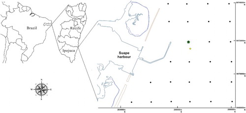
The experimental data were obtained using a wave buoy (Waverider MKIII buoy, Datawell BV, Netherlands), denominated UFPE01, which was moored over the continental shelf off the southern coast of the state of Pernambuco, in northeastern Brazil. The buoy was moored at a depth of 17 m at 286386.97m E, 9071447.47m N (UTM 25L, datum WGS84) (Figure 1).

Figure 1. Location of the buoy moored off Suape Harbor in Ipojuca, Pernambuco state, northeastern Brazil. The position of the UFPE01 buoy (yellow lozenge) and the DOW (Downscaling Ocean Waves) point (green), as described below. The black dots represent the model grid (1 km by 1 km).

The buoy has a built-in compass to determine magnetic north, and accelerometers to measure its movement, which characterises passing waves. The principal wave parameters were compiled for each hour of measurement. These parameters include significant wave height (H_S), peak period (T_P), and peak direction (D_P), calculated automatically by a program provided by the manufacturer with an accuracy of 0.5%.

The UFPE01 wave buoy measured the wave energy spectrum between October 2011 and November 2014, except for short periods when the buoy lost contact or was removed for maintenance. A total of 22,190 samples of directional wave spectrum data were collected during the period of the present study.

2.2. Overview of SMC-Brasil

The SMC is a set of programs, databases, and procedures designed to facilitate the analysis of wave-driven coastal processes. The project was developed with the collaboration of the Spanish Agency for Cooperation in International Development (AECID) and the Environmental Hydraulics Institute of the University of Cantabria. The Brazilian version of the SMC, known as SMC-Brasil, is an improved version of the system, developed initially for other countries, and includes recent scientific advances in coastal engineering and computer science. The SMC-Brasil package is composed of two main modules (Figure 2), one which permits the study of shore dynamics, and a second module (SMC-Tools) which runs data processing, creating statistical analyses from the databases of environmental variables, such as bathymetry, waves, and tides, which are included in the package.

Figure 2. Block diagram representing the main SMC-Brasil functions used in the present study.

One important function of SMC-Tools is to model the propagation of wave series from the ocean to the coast, which was the main function employed in the present study. This function permits the calculation of the waves at a point near the position of the buoy, as described in the following section.

The SMC-Tools module also permits the statistical processing of the wave data and the characterisation of the wave climate for any region off the Brazilian coast, based on the reanalysis of the 60 years of wave data stored in the database. For this, the Mathematical Analysis and Environmental Variables Statistics (Ameva) tool is used.

2.3. Calculating the wave climate with SMC-Brasil

The SMC-Brasil package includes an internal ocean wave database, known as Global Ocean Waves (GOW), which is based on a 60-year wave forecasting reanalysis, from 1948 to 2008. The Wavewatch III model (Tolman 2009) was used to model the waves in the Atlantic Ocean, with a resolution of 0.5° × 0.5°. The global reanalysis of the 10-m wind field data from NCEP/NCAR (available at http://www.ncdc.noaa.gov/data-access/model-data/model-datasets/reanalysis) was used as the input data for the wave model. The spatial resolution of the wind data was 1.9° × 1.9°, with a temporal resolution of 6 h.

The SMC-Brasil downscales the GOW reanalysis data, propagating waves from a theoretical point in deep oceanic waters toward shallow points where the influence of the ocean floor is more relevant. This is based on a shallow water wave model, called SWAN (Simulating Waves Nearshore), which computes the effects of the bottom on the waves. The downscaling was based on the same GOW wind data, which were adapted by the SWAN model to propagate waves toward points near the coast, known as DOW (Downscaling Ocean Waves) points, over a grid with a resolution of approximately 1 km × 1 km. The DOW point chosen as the wave energy source (Figure 1) is located at 286534m E, 9071845m N (UTM 25L, datum WGS84).

2.4. Spectral analysis and partitioning

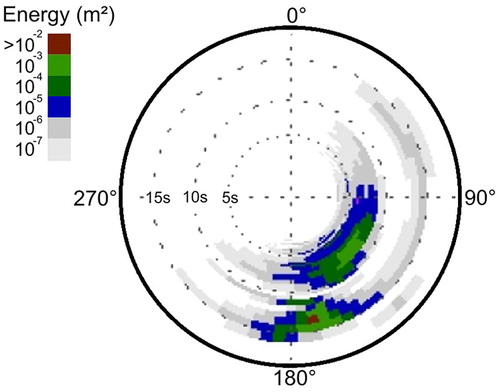
In most cases, an experienced observer can visually distinguish and partition the spectral distribution plot (Figure 3). However, it is necessary to automate the partitioning criteria to permit the continuous processing of the samples without the need for human intervention.

Figure 3. Spectral representation of the sea state over one hour of data collection.

The partitioning procedure was modified for the detection and elimination of misleading peaks, following Portilla et al. (2009), based on the following steps:

1. Use the frequency domain to detect every energy maximum, as well as every minimum located between each pair of maxima;

2. Eliminate the higher frequencies, corresponding to the tail of the energy spectrum, which vary excessively in relation to the wind sea energy. This cut-off occurs at a predetermined frequency, known as the ‘tail frequency’ (f_T). In the present study, a tail frequency of f_T = 0.35 Hz was used.

3. Bundle the energy bins located between the minima identified in step (i) in the initial partition set. It is also necessary to calculate the total energy of the spectral distribution, as well as the energy of each initial partition.

4. Determine the wind sea cut-off frequency (f_C) and peak frequency (f_P), as described in Section 2.5. The following steps are applied only to frequencies lower than f_C.

5. Discard partitions in which the peaks have less energy than both neighbouring partition peaks.

6. Discard partitions that have only one or two frequency bins between their minima.

7. Discard partitions with energy of less than 8% of the total energy.

The original partitioning method (Portilla et al. 2009) followed the steps presented above, with the exception of step 4, whose method is detailed hereafter.

2.5. Wind sea detection system

The determination of the cut-off frequency for the wind seas is based on the formula of Komen et al. (1984) (Equation (4)):(1) where U₁₀ is the wind speed at a height of 10 m above water level; β = 1.3 is the calibration factor; ψ is the wind direction; θ is the wave direction; ; f is the wave frequency.

The wind sea frequency range is related to the wind speed and direction, as described in the following equation:(2)

In order to determine the cut-off frequency, we consider that the wind seas are propagated in the same direction as the wind. As the cosine term of the equation is equal to 1, the minimum wind sea frequency (f_mw) is equal to:(3)

Wind speeds near the coast are statistically slower than those recorded over the ocean (Baptista 2003). An approach was developed to identify the energy peak that best represents the wind sea peak within the spectral distribution. In practice, this approach proved to be highly efficient for the detection of wind sea peaks. This approach consists of delimiting an area within which the spectral distribution is scanned for the point of highest wave energy (the modal value), which represents the wind sea peak. The minimum wind sea frequency (f_mw) delimits the area to be scanned, with the tail frequency (f_T) representing the maximum value (as in step (ii), above).

After determining the new peak frequency, the associated wind speed is determined by the JONSWAP spectrum (Sumer and Fredsøe 1997). The wind speed is determined by the association with this new peak frequency, as:(4) where x is the fetch in meters.

The algorithm then calculates a new minimum frequency for the wind seas, using the formula of the minimum wind sea frequency (Equation (3)). However, this minimum frequency does not always correspond to the minimum energy between neighbouring peaks (as described in step (i) above). The neighbouring frequencies are then scanned for an energy minimum, which will be considered to be the cut-off frequency, f_C (Figure 4).

Figure 4. (a) Sample of spectral sample from the buoy data, showing local wind speed and direction (red vector), and the frequencies calculated (red squares and arcs); (b) a new cut-off frequency, f_C (red arc), the wind sea system (W), the swell peak (orange square) and the swell system (S), as explained in the text.

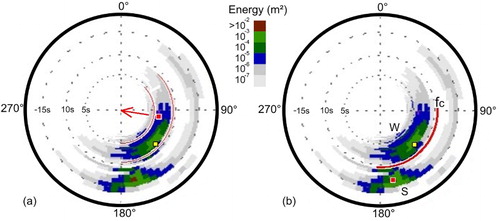
The initial peak frequency (the red square) and an initial cut-off frequency were calculated based on wind speed and direction (the red vector in Figure 4(a)). The area delimited by the initial cut-off frequency and the frequency tail (red arc) is then scanned for the new wind sea peak frequency (yellow square). In Figure 4(b), after determining a new cut-off frequency, f_C (red arc), the wind sea system (W) comprises all the energy delimited by the cut-off frequency (f_C). The next step is to determine the swell peak (orange square) and the swell system (S).

After delimiting the wind sea energy distribution by the cut-off frequency, the algorithm considers the wave energy peaks at lower frequencies as potential swell peaks, after which, it executes steps (v)–(vii) described at Section 2.4. These steps were adequate, in most cases, to effectively separate the swell system from the wind sea system and to bundle the swell energy into either a single system or two different systems.

3. Results

3.1. Characterisation of the wave climate using the buoy data

Table 1 shows the extreme and mean values (avg.) of the wave parameters and their standard deviations (std.) per year, as well as for the entire series. The years have very similar average values, with the exception of 2011, which is represented only by the austral spring months (October–December), in contrast with the other years, which include all the different seasons.

Table 1. Descriptive statistics of the typical and extreme wave climates, that is, the averages (avg.) and standard deviations (std.) of the principal wave parameters: significant wave height (H_S), peak period (T_P), and peak direction (D_P), for each year and the entire dataset.

	HS (m)				TP (s)				DP (degrees)
Year	Min.	Max.	Avg.	Std.	Min.	Max.	Avg.	Std.	Min.	Max.	Avg.	Std.
SSeries	00.72	22.85	11.48	00.326	44.35	220.00	88.8	22.10	662	2236	1138	116.9
22011	11.04	22.62	11.57	00.257	55.00	115.38	99.0	11.87	1101	1190	1143	115.7
22012	00.85	22.80	11.48	00.333	44.55	118.18	88.6	11.97	886	2236	1136	115.5
22013	00.72	22.57	11.45	00.320	44.35	118.18	88.9	22.18	662	1194	1137	118.6
22014	00.76	22.85	11.49	00.352	44.35	220.00	99.1	22.32	993	2204	1139	117.4

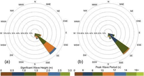
The directional characteristics of the wave climate indicate that most (over 60%) of the wave energy comes from the southeast quadrant, with smaller portions coming from the south-southeast and east-southeast quadrants (around 15% each), with the remaining 10% coming from the southern quadrant (Figure 5).

Figure 5. (a) Significant wave heights (H_S) and (b) peak period (T_P) directional roses, calculated for the wave data collected by the UFPE01 buoy (entire dataset).

3.2. Wind seas and swell

We obtained a more detailed overview of the region's wave climate through the analysis of the partitioned spectral energy wave data (Figure 6). This analysis reveals the relationship between each system (wind seas and swell) and the directional pattern of the wave climate.

Figure 6. Means and standard deviations of the significant wave heights and the primary period for the swell and wind sea partitions, and for the total energy spectrum.

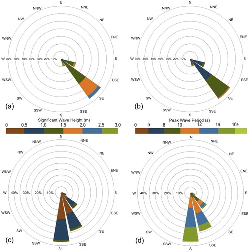
Most (approximately 65%) of the wind sea energy comes from the southeast quadrant (Figure 7(a,b)), while a further 20% comes from the east-southeast quadrant, and approximately 10% from the south-southeast quadrant, with peak periods of mostly 10 s or less. The swell energy (Figure 7(c,d)) was mostly derived from the south and south-southeast quadrants, with another 10%, approximately, coming from the southeast quadrant. The swell waves typically had a significant height of less than 1 m, with peak periods ranging between 10 and 16 s.

Figure 7. Roses of significant wave height and peak period, representing the energy of wind seas (a and b) and swell (c and d) for the entire dataset.

Nearly one-third of all the wind sea energy comes from the southeast quadrant, with around one-fifth from east-southeast, and approximately one-tenth from the south-southeast quadrant. The probability density function (PDF) of the distribution of the energy among these primary axes indicates that the wind sea energy is concentrated mainly between 100° and 170°, while the swell energy is mainly above 130° (Figure 8). The probability of a sample having a primary direction equal to or less than 155° is 86.4%, while 13.6% of samples have a primary direction of over 155°.

Figure 8. Probability density function showing the percentages of the total energy (solid grey line), wind sea (dotted line), and swell systems (dashed line) for the entire dataset, based on the distribution of the peak direction.

3.3. Characterisation of the wave climate using SMC-Brasil

The DOW point, located at coordinates 287534m E and 9071845m N (UTM 25L, datum WGS84), was the extraction point of the wave data (Figure 1). The wave climate at this point (Table 2; Figure 9) indicates a probability of more than 75% for waves from the east-southeast and 24.11% for waves from the southeast. The other 0.55% of waves arrive from the east, and a diminutive percentage (0.08%) from the south-southeast.

Figure 9. The directional rose of significant wave height (H_S) at the DOW point, calculated using the wave data from SMC-Brasil database.

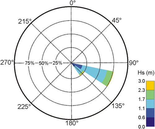
Table 2. The wave climate probabilities calculated using the wave data (Direction, H_S50%, H_S12, T_P50%, T_P12) from SMC-Brasil database.

Direction	Probability (%)	HS50% (m)	HS12 (m)	TP50% (s)	TP12 (s)
ENE	0.00	1.11	1.13	9.51	10.98
E	0.55	0.90	1.78	7.06	10.97
ESE	75.25	1.37	2.59	7.46	12.12
SE	24.11	1.37	2.48	6.65	8.41
SSE	0.08	1.25	1.86	5.36	11.04

Note: There is a probability of more than 75% of the waves coming from the east-southeast

The mean (or typical) significant wave height (the heights recorded in 50% of the records: H_S50%), and the height of storm (or extreme) waves, which are recorded as extreme events, occurring during only 12 h per year (H_S12), and the corresponding wave period values (recorded in 50% of the time (T_p50%) and recorded as extreme events, occurring during 12 h per year (T_p12), are shown in Table 2.

3.4. Comparison of the climates obtained from the buoy data and the SMC-Brasil database

For the first comparison, we used the PDF of significant wave heights (H_S), superimposing the buoy wave climate over those obtained from the SMC-Brasil database (Figure 10(a)). Both curves are very similar, and the modal value is approximately 1.3 m. The buoy data presents a higher frequency of waves with H_S values of over 1.8 m, while the SMC-Brasil database presets a higher frequency of waves with H_S values lower than 1.4 m.

Figure 10. Comparisons between the (a) H_S, (b) T_P, and (c) D_P values recorded by the wave buoy (orange line) and those derived from the SMC-Brasil database (vertical bars). The images are superimposed, and the values of each scale coincide. (d) Probability density functions of the peak periods associated with the H_S12 according to SMC-Brasil database.

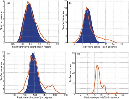
Comparing the PDFs of the peak period (T_P), there is a high degree of similarity between the two datasets (Figure 10(b)) in the range of periods of less than 7.0 s. The modal points of both curves are very close, at around 7.0 s. For the values of peak periods longer than 7.0 s, a slight difference begins to appear between the curves, with the probabilities of the SMC-Brasil data being concentrated near this modal value, corresponding to a more normal distribution curve, with a very small probability of the occurrence of wave periods of over 10.0 s. The wave climate defined by the buoy data is quite distinct, with a very steep decrease in the 7.0 s modal value, but less steeply above 9.0 s, with a reasonable probability of waves with peak periods of between 10.0 and 14.0 s. This range corresponds exactly to the occurrence of swell waves.

However, by analysing the PDFs of the peak periods (T_P) associated with the larger waves that occur during 12 h per year, i.e. the H_S12 (Figure 10(d)), a minor peak can be observed in the mode at around 11 s, which corresponds approximately to the energy that appears in the PDF of the buoy data related to the swell systems. These systems appear to be visible in the wave climate of SMC-Brasil only in the case of extreme events, indicating that the detection of lower wave height events was unsatisfactory.

The PDFs of peak direction (D_P) present the greatest differences between the SMC-Brasil wave climate and that derived from the UFPE01 buoy data (Figure 10(c)). There is a clear displacement of the wave buoy data to the right, in comparison with the SMC-Brasil wave data.

While the SMC-Brasil curve presents a modal point of approximately 120°, the wave buoy presents a curve with a peak at 125°. The difference between these peaks is negligible, and may reflect the need for the calibration of the buoy compass to the magnetic north, for example. Given this, the buoy data are offset slightly to the left, so that the peak coincides with that of the SMC-Brasil data, reinforcing their similarities, similar except for the third modal point observed in the buoy data near 170°.

This third peak corresponds exactly to the swell systems, as shown in Section 3.2 and Figure 7. When comparing the peak direction PDFs, then the swell systems are clearly underestimated by the SMC-Brasil data, but can be identified clearly in the data from the UFPE01 wave buoy.

The calibration of the model uses satellite scatterometer data. However, Chen et al. (2002) showed that this does not always calibrate the swell data adequately, which may account for the differences between the datasets identified in the present study. This type of calibration may account for the underestimation of the presence of swell by the SMC-Brasil model.

4. Discussion

The wave climate of the region off the southern coast of the Brazilian state of Pernambuco was determined by the spectral distribution of the waves recorded by the directional wave buoy and analysed using the partitioning method modified from Portilla et al. (2009). As the buoy was moored at the transition between deep and shallow waters (17 m), depth effects such as refraction, shoaling, and bottom friction would have influenced the waves (Vincent and Briggs 1989).

The prevailing trade winds in the tropical South Atlantic basin are southeasterlies (Baptista 2003). As expected, higher levels of wave energy deriving from the southeast, and reduced wave energy from the south (swell system) is clear from the buoy data, given that only around 10% of the wave energy was recorded from the south.

Pianca et al. (2010) analysed 11 years of NOAA GFS reanalysis data using a Wavewatch III (Tolman 1989) model to calculate the wave climate at an oceanic forecast point in deep water (4600 m) at approximately 150 km east-southeast of the UFPE01 mooring. The results were similar to those of the present study, except for the presence of northern swells. These northern swells, predicted by the model in the deep ocean, mostly during the summer and spring months, were generated by major storm activity over the North Atlantic Ocean, and were not detected by the UFPE01 buoy due to its relatively sheltered coastal location.

The wave climate obtained from the downscaling of the reanalysis wave data from the SMC-Brasil software package was broadly consistent with those recorded by the UFPE01 directional wave buoy, in particular in the distribution of wave heights. The SMC-Brasil wave climate nevertheless underestimated the swell systems, which were only recorded during extreme swell events. This difference is meaningful, and should be taken into account in future studies using the SMC-Brasil package, primarily by selecting sea states that emphasise swell systems, i.e. waves with peak periods of over 10 s and a direction of more than 150°.

The results of the wave climatology approach developed in the present study may be useful for the calibration of data in further wave forecast reanalyses. This could be applied in future versions of the SMC-Brasil database, as well as in other types of study that require a reliable wave climatology of the tropical region of South America.

5. Conclusion

The wave climate of the study region, measured by the UFPE01 buoy, was characterised by a predominance of southeast wind seas with peak periods of up to 10 s, driven by the trade winds blowing over a large catchment area of the tropical Atlantic Ocean. Southern quadrant swells with peak periods of over 10 s were also present, created mainly by storms over the sub-tropical and temperate Atlantic Ocean.

Comparisons between the results of the Wavewatch III modelling of the NOAA GFS wind data and the data collected by the UFPE01 wave buoy revealed a high degree of similarity, once the differences in the depth of the data collection sites are taken into account. This reinforces the findings on the wave climate of the study region, presented here.

However, the SMC-Brasil wave climate clearly underestimated the low amplitude swell systems. The absence of swell systems in the climatology of the SMC-Brasil was presumed to have been related to the calibration of the reanalysis data, which was based only on satellite scatterometry. In this approach, the detection of low swell systems is hampered where wind wave systems predominate. Given this, more reliable results would be obtained from wave simulation models that are calibrated using data collected in situ.

The findings of this study emphasise the importance of nearshore data from the coast of northeastern Brazil, where the selection and calibration of numerical models will be fundamental to the success of future coastal management research and practices.

Acknowledgements

The financial grant received from CNPq, FACEPE, Suape Port, and Rede Ondas supported the acquisition and maintenance of the wave buoy used to collect the data analysed here. We thank the editor and two anonymous reviewers for their valuable contributions to this paper.

Disclosure statement

No potential conflict of interest was reported by the authors.

ORCID

Gabriel Gomes http://orcid.org/0000-0001-8969-3605

Alex Costa da Silva http://orcid.org/0000-0002-5828-3598

Additional information

Funding

The authors would like to thank Conselho Nacional de Desenvolvimento Científico e Tecnológico (CNPq) [Proc:. 558 139/2009-4]; Fundação de Amparo à Ciência e Tecnologia do Estado de Pernambuco (FACEPE) [Proc.: APQ-1056-1.08/15] for financing the project Monitoring Wave Climate in the Northeast of Brazil.

References

- Baptista MC. 2003. Uma análise do campo de vento de superfície sobre o oceano atlântico tropical e sul usando dados do escaterômetro do ers. [place unknown]: INPE.
- Chen G, Chapron B, Ezraty R, Vandemark D. 2002. A global view of swell and wind sea climate in the ocean by satellite altimeter and scatterometer. J Atmos Oceanic Technol. 19:1849–1859. doi: 10.1175/1520-0426(2002)019<1849:AGVOSA>2.0.CO;2
- Feng X, Tsimplis MN, Quartly GD, Yelland MJ. 2014. Wave height analysis from 10 years of observations in the Norwegian Sea. Cont Shelf Res. 72:47–56. doi: 10.1016/j.csr.2013.10.013
- Gomes G, Silva AC. 2014. Coastal erosion case at Candeias Beach (NE-Brazil). In: Silva R, Strusińska Correia A, editors, Coastal erosion and management along developing coasts: selected cases. J Coastal Res, Special Issue. 71:30–40.
- González M, Nicolodi JL, Quetzalcóatl O, Cánovas V, Hermosa AE. 2016. Brazilian coastal processes: wind, wave climate and sea level. In: Short AD, Klein AH da F, editors, Brazilian Beach Systems, Coastal Research Library 17. Springer; p. 37–66. ISBN 978-3-319-30392-5.
- Hauser D, Kahma K, Krogstad HE, Lehner S, Monbaliu JAJ, Wyatt LR. 2005. Measuring and analysing the directional spectra of ocean waves – Working Group 3. COST off., EU Publications Office (OPOCE), ISBN: 92-898-0003-8; 465pp.
- Komen GJ, Hasselmann S, Hasselmann K. 1984. On the existence of a fully developed wind–sea spectrum. J Phys Oceanogr. 14:1271–1285. doi: 10.1175/1520-0485(1984)014<1271:OTEOAF>2.0.CO;2
- Laing AK, Gemmill W, Magnusson AK, Burroughs L, Reistad M, Khandekar M, Holthuijsen L, Ewing JA, Carter DJT. 1998. Guide to wave analysis and forecasting. 2nd ed. WMO No. 702. Geneva: World Meteorological Organization.
- Lionello P, Günther H, Hansen B. 1995. A sequential assimilation scheme applied to global wave analysis and prediction. J Mar Syst. 6:87–107. doi: 10.1016/0924-7963(94)00010-9
- Nakicenovic N, Alcamo J, Davis G, de Vries B, Fenhann J, Gaffin S, Gregory K, Grübler A, Jung TY, Kram T, et al. 2000. Special report on emissions scenarios: a special report of Working Group III of the Intergovernmental Panel on Climate Change. [place unknown]: Intergovernmental Panel on Climate Change.
- Pianca C, Mazzini PLF, Siegle E. 2010. Brazilian offshore wave climate based on NWW3 reanalysis. Brazilian J Oceanogr. 58:53–70. doi: 10.1590/S1679-87592010000100006
- Portilla J, Ocampo-Torres FJ, Monbaliu J. 2009. Spectral partitioning and identification of wind sea and swell. J Atmos Ocean Technol. 26:107–122. doi: 10.1175/2008JTECHO609.1
- Reguero BG, Menéndez M, Méndez FJ, Mínguez R, Losada IJ. 2012. A Global Ocean Wave (GOW) calibrated reanalysis from 1948 onwards. Coast Eng. 65:38–55. doi: 10.1016/j.coastaleng.2012.03.003
- Semedo A, SušElj K, Rutgersson A, Sterl A. 2011. A global view on the wind sea and swell climate and variability from ERA-40. J Clim. 24:1461–1479. doi: 10.1175/2010JCLI3718.1
- Sumer BM, Fredsøe J. 1997. Hydrodynamics around cylindrical structures. Vol. 12. Advanced Series on Ocean Engineering. Singapore: World Scientific.
- Sverdrup HU, Munk WH. 1947. Wind, sea, and swell. theory of relations for forecasting. Washington (DC): United States Navy Department - Hydrographic Office.
- Tolman HL. 1989. The numerical model WAVEWATCH: a third generation model for the hindcasting of wind waves on tides in shelf seas. Communications hydraulic geotechnical engineering. Delft: Delft University of Technology. Report No.: 89–2, 72.
- Tolman HL. 2009. User manual and system documentation of WAVEWATCH III version 3.14. NOAA/NWS/NCEP/MMAB Technical Note 276, 194 pp.+ Appendices.
- Vincent CL, Briggs MJ. 1989. Refraction-diffraction of irregular waves over a mound. J Waterway Port Coastal Ocean Eng. 115(2):269–284. doi: 10.1061/(ASCE)0733-950X(1989)115:2(269)