Operational system for automatic coastal upwelling detection in the Baltic Sea based on the 3D CEMBS model

ABSTRACT

The upwelling in the Baltic Sea region is very common phenomenon. According to different studies, in some places it can exist almost one-third of the year leading to vertical mixing and transporting fresh, rich in nutrients water from deeper layers to the surface. The upwelling phenomenon has been analysed for years 2010–2016, during thermally stratified period, i.e. between May and September. Surface layer temperature from coupled ecosystem model of the Baltic Sea – 3D CEMBS was analysed together with NOAA/AVHRR satellite SST observations. Wind data from weather forecasting model – UM from ICM UW were also analysed to describe favourable conditions for the upwelling occurrences. The research includes statistical analysis of entire Baltic Sea region as well as particular examples from selected areas. Areas of upwelling occurrences were found along almost entire coastline of the Baltic Sea. Main areas were located along Swedish coast in Baltic Proper, Oland and along Finnish coast in the Gulf of Finland, where the event can last up to 30% of the time. Other areas, with frequencies over 20%, include Polish coast, Gotland and Bay of Bothnia. It was determined that collected results were in good agreement with earlier studies, with satellite data giving slightly higher frequencies closer to the shore. Based on these results, an automated coastal upwelling detection system was designed and launched in operational mode together with the 3D CEMBS model.

KEYWORDS:

• Upwelling
• Baltic Sea
• operational modelling

Introduction

Coastal upwelling is a phenomenon of deep water's uplift to the surface layer that occurs under certain conditions and is driven by wind and the Corriolis effect. The net transportation of water in the surface layer is perpendicular to wind direction. This is called the Ekman transport. According to Ekman theory, it is directed to the right on the northern and to the left on the southern hemisphere. If the wind blows parallel to the coastline, the water from the Ekman layer is pushed away from the coast. Cooler and usually rich in nutrients water from deeper layers is carried up to the surface. This deep water replenishes the euphotic zone stimulating the growth of primary producers, often resulting in rapid blooms.

The Baltic Sea is relatively small and very specific basin (Figure 1). It is regularly replenished with saline, rich in oxygen water flowing in from the North Sea through Danish straits. On the other hand, many rivers that drain into the Baltic Sea constantly deliver rich in nutrients freshwater. Permanent salinity layer, river runoff and seasonal changes of temperature contribute to very strong stratification of the Baltic Sea (Vopio 1981). Due to a relatively complex coastline, wind from any direction may lead to occurrence of coastal upwelling. This in turn causes vertical mixing of the water column. The extent of upwelling for the Baltic Sea can reach up to 20 km offshore (Gidhagen 1987) and is determined by the internal Rossby radius, which for the Baltic Sea ranges from 2 to 10 km (Fennel et al. 1991; Osiński et al. 2010). During summer and autumn, when the water from the surface layer is warm and thermal stratification is most distinct, upwelling can lead to significant drop in temperature by more than 10°C (Lehmann and Myrberg 2008). Horizontal gradient of surface temperature resulting from upwelling can reach 5°C km−1 (Krężel et al. 2005). This gives the possibility of detection of this phenomenon through temperature measurements by various means (e.g. in situ measurements, using space-borne instruments) or model calculations. In some areas of the Baltic Sea, upwelling is very common and can last up to a month. There are also areas where upwelling can exist for up to one-third of the time (Gidhagen 1987). The influence of upwelling on surface temperature, mixing of water column and replenishment of nutrients in the surface layer renders the investigation of this phenomenon important. The commonness and the reach of upwellings on the Baltic Sea lead to many theoretical, empirical and computational studies (Gidhagen 1987; Bychkova et al. 1988; Jankowski 2002; Myrberg and Andrejev 2003; Krężel et al. 2005; Lehmann and Myrberg 2008; Lehmann et al. 2012) just to name a few.

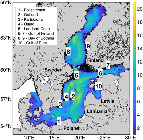
Figure 1. Location of studied upwelling areas.

Many automatic methods of upwelling detection have been developed and tested. Many of these methods utilise SST observations, mainly from satellites. These methods are based on specific visual characteristics of upwelling and try to identify the event by applying different image segmentation and clustering techniques (Marcello et al. 2005; Nascimento et al. 2012; Tamim et al. 2014) or neural networks (Chaudhari et al. 2008). Other methods together with SST use also meteorological data, e.g. wind measurements from buoys, meteorological models or microwave sensors (Plattner et al. 2006, Li et al. 2012). Myrberg and Andrejev (2003) proposed different approach that was used for the Baltic Sea. It is based on the results of hydrodynamic models and focuses on persistency of vertical velocity to define an upwelling index, instead of using changes of surface temperature. Taking advantage of latitudinal gradient that characterises SST in the Baltic Sea, Lehmann et al. (2012) proposed yet another method of upwelling detection following research by Bychkova (1988).

This paper presents the results of applying the latter method together with results from NOAA/AVHRR satellite measurements, results from 3D Coupled Ecosystem Model of the Baltic Sea – 3D CEMBS (Dzierzbicka-Głowacka et al. 2013a, 2013b) and wind conditions from Unified Model (UM) from Interdisciplinary Centre for Mathematical and Computational Modelling, University of Warsaw (ICM UW) (Herman-Iżycki et al. 2002). It extends previously conducted upwelling research carried out over past decades. These studies include localisation and analysis of 22 upwelling areas in the Baltic Sea (Bychkova et al. 1988), based on satellite data from years 1980 to 1984 and similar study by Lehmann et al. (2012) based on SST data from satellite measurements and BSIOM model, as well as wind conditions covering years 1990–2009.

Maps of daily mean temperature based on satellite and model data were used to determine the presence and properties of upwellings during the period from May to September, when the thermal stratification of the sea is very strong. Mean values for each month, each year as well as mean upwelling frequency for the entire period were calculated. Wind data obtained from the UM were used to show atmospheric conditions for the upwelling to take place. The study covers years 2010–2016 and presents results from the entire Baltic Sea. Promising results of combining automated upwelling detection methods with forecasting capability of 3D CEMBS led to the development of automated detection system that provides forecasts for coastal upwellings in the Baltic Sea in the operational mode.

Material and methods

SST data

One of main features that determine the upwelling occurrence is uplift of deep water to the surface. During thermally stratified period of the year in the Baltic Sea, this is indicated by rapid drop in sea surface temperature. This drop can be detected by satellite measurements as a cold area of SST in the coastal zone. To assess these events’ frequency and spatial distribution, sea surface temperature measured by AVHRR instrument was used together with model computations. Satellite data were processed using DESAMBEM algorithms (Woźniak et al. 2008). The algorithm was validated (Darecki et al. 2008) and used in automated monitoring system of the Baltic Sea developed within the SatBałtyk project (Ostrowska et al. 2015). Spatial resolution of satellite data is 1 km and depending on atmospheric conditions there can be up to several such scenes per day. 3D CEMBS is a coupled ecosystem model developed in the Ecohydrodynamics Laboratory, IO PAS (Dzierzbicka-Głowacka et al. 2013a, 2013b). It consists of active ocean, ecosystem and ice modules which calculate wide range of parameters, e.g. water temperature, salinity, currents, sea level, sea ice coverage, concentration of various nutrients, chlorophyll-a, zooplankton and many others. Passive land module provides input data such as freshwater inflow and nutrient discharge from rivers. Weather forecasts from UM are used as forcing data on the boundary layer. UM computes 72-hour forecasts, four times a day, providing information about necessary atmospheric parameters. Horizontal resolution of 3D CEMBS is 1/48°, which corresponds to ca. 2.3 km grid. Vertically model is divided into 21 layers and the thickness of layers increases with depth. The operational version of 3D CEMBS was launched in 2012 and has been developed further (Dzierzbicka-Głowacka et al. 2013c), e.g. data assimilation from AQUA/MODIS satellite has been introduced (Nowicki et al. 2015), ecosystem module parameterisation is constantly enhanced. ICE The accuracy of temperature from both sources, used in this study was estimated, based on in situ measurements from International Council for the Exploration of the Sea (ICES) database, to ca. 1.2°C.

Wind data

Wind data used for analysis were calculated by the UM weather forecasting model. Wind at 10 m height was extracted for eight selected areas, where upwelling is most frequent (Figure 1). There are five locations in the Baltic Proper: near Polish coast, Gotland, Karlskrona, Oland and near Landsort Deep, two along north and south coasts of the Gulf of Finland and one in the Bay of Bothnia. Daily mean values were used for the analysis.

Methodology

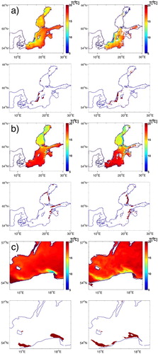
Satellite and model data were compared based on automatic upwelling detection method (Lehmann et al. 2012). The method assumes that during the upwelling, water from below thermocline reaches the surface, causing significant drop in temperature. Therefore, this method is only able to detect strong coastal upwelling events during stratified period of the year. Daily mean values of temperature were calculated for years 2010–2016. Temporal resolution of data is one day. Based on the assumption that there is a latitudinal SST gradient from the south to the north, following Bychkova (1988) and Lehmann et al. (2012), whole Baltic Sea was divided into latitudinal zones. Mean temperature was calculated for each zone. Upwelling was detected, if temperature at a specific pixel differed from corresponding mean by more than a threshold of 2°C. For some regions, instead of using latitudinal zones, one mean temperature was calculated independently for each of them. In particular, Gulf of Finland, Gulf of Riga and part of Bay of Bothnia. Having one mean temperature for a particular area instead of multiple latitudinal zones improved upwelling detection in aforementioned regions. However, this sometimes led to erroneous detection of upwelling events near the entrance to the Gulf of Finland and Gulf of Riga and in the north part of the Bay of Bothnia. These results are excluded from further analysis. As a result of the above process, datasets of 1071 model scenes and 1013 satellite scenes were created. Data were analysed visually to validate the method. Example of validation results is presented in Figure 2. The left and right parts of each figure represent model and satellite data, respectively. The upper side presents raw SST data on model grid, and the lower, upwelling areas detected by the algorithm. Figure 2(a) presents upwelling event that took place on 13.09.2011. Figure 2(b) shows multiple upwelling areas on 22.07.2013. Figure 2(c) presents upwelling from 18.08.2015. One can see that the automated detection results are in good agreement with visually observed upwelling zones on the SST maps. Model results are also consistent with satellite measurements. Events presented in Figure 2(a,b) were selected for sample case studies later in this paper. These examples were selected to show that there are many areas where upwelling is present aside from the eight selected for further analysis.

Figure 2. Sample upwelling detection scene. 13.09.2011 (a), 22.07.2013 (b), 18.08.2015 (c). Left – model, right – satellite. Upper – SST, lower – upwelling presence.

Based on these data, a set of maps was prepared, including percentage of upwelling days for each year, monthly averages and overall upwelling frequency calculated for the entire studied period. Because the study is about coastal upwelling, mask excluding open sea was generated automatically for distance greater than 15 grid cells, ca. 35 km, from any coast.

Time series of surface temperature from selected locations were analysed. Model data were compared with satellite measurements. Time series were also visually analysed to confirm proper functioning of detection algorithm. To achieve better coverage of satellite data each point was set to have size 3 × 3 pixels.

Upwelling detection can be treated as a binary classification problem, where model identifies presence or absence of upwelling at a given point. Therefore, several statistical measures were calculated to give a better quantitative description of the performance of proposed method. Results for each of the eight sample locations are presented in Table 2. Relevant equations for each of the statistics are:

True Positive Rate:$\mathrm{T}\mathrm{P}\mathrm{R}=\mathrm{T}\mathrm{P}/\mathrm{P}$True Negative Rate:$\mathrm{T}\mathrm{N}\mathrm{R}=\mathrm{T}\mathrm{N}/\mathrm{N}$Positive Predictive Value:$\mathrm{P}\mathrm{P}\mathrm{V}=\mathrm{T}\mathrm{P}/\left(\mathrm{T}\mathrm{P}+\mathrm{F}\mathrm{P}\right)$Negative Predictive Value:$\mathrm{N}\mathrm{P}\mathrm{V}=\mathrm{T}\mathrm{N}/\left(\mathrm{T}\mathrm{N}+\mathrm{F}\mathrm{N}\right)$Accuracy:$\mathrm{A}\mathrm{C}\mathrm{C}=\left(\mathrm{T}\mathrm{P}+\mathrm{T}\mathrm{N}\right)/\left(\mathrm{P}+\mathrm{N}\right)$F1-score:$\mathrm{F}1=\left(2\ast \mathrm{P}\mathrm{P}\mathrm{V}\ast \mathrm{T}\mathrm{P}\mathrm{R}\right)/\left(\mathrm{P}\mathrm{P}\mathrm{V}+\mathrm{T}\mathrm{P}\mathrm{R}\right)$where TP – true positive, TN – true negative, FP – false positive, FN – false negative, P – number of upwellings detected by satellite data, N – number of days without upwelling according to satellite data.

Wind data at 10 m height were also analysed in all locations mentioned above. For each location percentage of days with favourable winds was calculated by establishing orientation of coastline. It was assumed that to induce upwelling, wind must blow parallel to the coast, at least 3.5 m s−1 for 2 days or longer (Bychkova et al. 1988). Received results were then compared with upwelling days resulting from SST data.

Results of method assessment

This study covers data from 2010 to 2016, from thermally stratified period, i.e. from May to September. During this period, there are 153 days, which gives a total of 1071 days. Model calculations provide continuous data resulting in 1071 analysed SST scenes for the whole Baltic Sea area. This means that frequency of 10% corresponds to the presence of upwelling for 107 days. Data from satellites are not always available due to atmospheric conditions, e.g. cloud coverage. This results in less frequent data. However, there can be several SST images per day. Combining these images resulted in 1013 scenes. Most of these scenes cover the area partially, which makes it more difficult to determine presence of upwelling. The average number of days with satellite data for a given point was 692 and was relatively equally distributed over the whole area. This means, that for each point ca. 65% of time series was covered.

Sample upwelling case study

Following section presents case study of two upwelling events presented in ‘Methodology’ section as examples of visual validation of the method (Figure 2a and b), i.e. upwelling event along Oland that took place in September 2011 and upwelling along east coast of Bay of Bothnia from July 2013. Location of each event is presented as points 4 and 9 in Figure 1. The choice of these events was arbitrary and was aimed to present sample results. However, analogous analysis was performed for several other cases with similar results. Time series of surface temperature and wind directions for each of these events are presented in Figure 3(a,b). Wind direction is presented in the upper part of each figure and favourable wind direction for each location is presented in the lower right part. SST series is presented in lower part. Satellite and model results are red and green respectively. Bars below temperature series represent upwellings. Red bar means that there was no upwelling at that time, green bar indicates presence of upwelling and ‘x’ means lack of data.

Figure 3. SST and wind time series of cases study from September 2011 (a) and July 2013 (b). Upper part represents wind time series. Lower part shows surface temperature. Red dots – model, green dots – satellite. On the lower bar: green – upwelling, red – no upwelling, ‘x’ – no data.

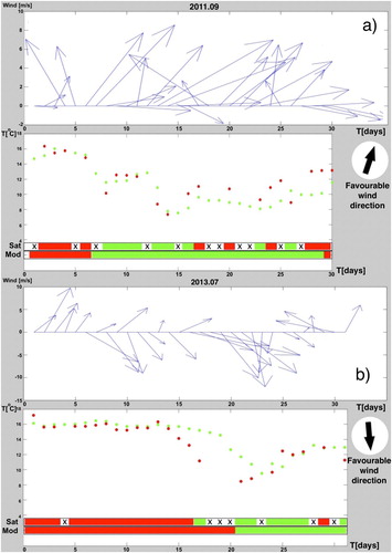
According to results derived from model data, first upwelling took place between 7th and 29th of September 2011. During that time, surface temperature decreased from 15°C to 7°C. Satellite observations provided similar results. However, scares satellite data after September 17th produced ambiguous results for that period. This result is consistent with wind data. Before 6th of September either wind direction was unfavourable or its magnitude to low. After that day, wind strengthened up to 10 m/s and its direction maintained favourable for most of the time, changing to western at the end of the month, which was followed by disappearance of upwelling and increase of surface temperature.

The second upwelling took place in the second half of July 2013. Satellite measurements produced positive signal of upwelling presence on July 17th but were unavailable for next 3 days. Upwelling derived from model data was detected on 20th of July and lasted till 2nd of August. Similarly to previous case, strong northern winds lasting for several days lifted cold water from deeper layers resulting in temperature drop from 16°C to 9°C. After 25th of July, the wind changed direction, thus stopping upwelling. However, its results were still visible through lower surface temperature for next few days.

Upwelling frequencies for years 2010–2016

Mean upwelling frequency distribution between May and September for the entire period of the study was calculated (Figure 4). Model and satellite results are presented on the left and right, respectively.

Figure 4. Mean upwelling frequency distribution between May and September for 2010–2016. Left – model, right – satellite.

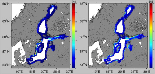
It can be seen (Figure 4) that main areas of upwelling events detected from satellite and model data are in good agreement. They also correspond well with the results of previous studies (Bychkova et al. 1988; Lehmann et al. 2012). Main areas of strong upwelling events can be found along Swedish coast and in the Gulf of Finland. As seen from model results, frequency of upwelling along the west coast of the Baltic Sea reaches 30% in the area near Landsort Deep and further south as well as up to 25% along the eastern side of Oland. In the Gulf of Finland, the phenomenon can be detected almost 23% of the time. It is also visible on both sides of Gotland. Less frequently, ca. 5% upwelling is also present along the coast of Lithuania and Latvia and in the Gulf of Riga. Upwelling is also observed in the Bay of Bothnia and along the Polish coast, where it reaches up to 20%. However, this is better visible from satellite measurements. There is also area of high frequency visible in the entrance to Gulf of Riga, which is much less visible in model data. In general, results from satellite and model are in good agreement. However, upwelling areas determined based on model data extend further from the coasts but are less frequent. Satellite results show areas of very high upwelling frequencies very close to the coast, which are less visible in model results. Table 1 presents comparison of upwelling frequencies derived from model and satellite data from selected locations (Figure 1). It also contains percentage of days with favourable winds, which will be discussed in part 3.3 of this paper. Upwelling frequencies derived from satellite measurements are higher than those derived from model calculations. Average difference between satellite and model results is 5.6 pp., which corresponds to 60 days out of total of 1071 days. As mentioned earlier, highest discrepancy can be observed near the Polish coast. The best agreement between model and satellite results can be observed in location 5, near Landsort deep, where upwelling was present over 30% of the time. This means that the upwelling in this area was present for 321 days.

Table 1. Percentage of upwelling and favourable wind days.

Location	Satellite (%)	Model (%)	Wind (%)
1	21.2	8.5	15.4
2	22.4	17.7	20.4
3	23.7	20.5	19.2
4	29.9	25.2	23.1
5	31	30.2	29.5
6	21.3	14.2	13.4
7	28.9	22.7	22.5
8	16.5	11.1	17.5

Taking satellite data as indicating actual events, and being a baseline for the model results we can explain the indexes calculated as follows. TPR measures the proportion of actual upwelling events that are correctly detected. TNR measures the proportion of non-upwelling days that are correctly detected. PPV and NPV are the proportions of positive and negative results that are true positive and true negative results, respectively. From Table 2, one can see that measures related to negative scenarios (non-upwelling days), i.e. TNR and NPV yield much more accurate results than the ones related to detected upwelling events. This means that proposed method applied on model data, in its current setup deals much better with detecting the absence of upwelling than upwelling events. This also means that the model tends to underestimate frequency of upwelling events, which is consistent with previous conclusions. The ACC varies from 0.75 in the fifth area, near Landsort deep, up to 0.91 in area 2, near Gotland. Mean accuracy is 0.83, which is very satisfying result. However, this statistical measure might be misleading for data that are not equally distributed. With upwelling events, this is exactly the case. As previously stated and presented in Table 1, depending on the area, upwelling events are present between ca. 10% and 30% of the time. Since the method is more likely to give false negative than false positive result the ACC measure is not best suited for its assessment. Instead, a more suitable measure is used. F1-score is a harmonic mean of TPR and PPV. As shown in Table 2, it is substantially lower than ACC with mean value of 0.57.

Table 2. Statistics of upwelling detection tool.

Location	TPR	TNR	PPV	NPV	ACC	F1
1	0.37	0.96	0.73	0.82	0.81	0.49
2	0.67	0.94	0.61	0.95	0.91	0.63
3	0.61	0.93	0.76	0.87	0.84	0.67
4	0.69	0.88	0.68	0.88	0.83	0.69
5	0.66	0.79	0.57	0.84	0.75	0.61
6	0.48	0.91	0.55	0.88	0.82	0.51
7	0.51	0.86	0.34	0.92	0.81	0.41
8	0.42	0.97	0.74	0.90	0.88	0.53
Mean	0.55	0.90	0.62	0.88	0.83	0.57

Spatial map of upwelling's frequency, for each year separately was prepared (Figure 5). In year 2010, there were strong and frequent (up to 31%) upwelling events along Swedish coast and near northern coast of the Gulf of Finland. There are also many areas with upwelling frequencies less than 10% distributed along almost all coasts. Satellite data also show upwelling areas in the Bay of Bothnia and entrance to the Gulf of Riga, ca. 22%. In 2011, frequency of upwelling increased along western coast of Baltic and near southern coast of Gulf of Finland reaching over 32%. Both satellite and model data show significant increase in upwelling frequencies south to Gotland ca. 27% and at the entrance to the Gulf of Riga 24%. There is also decrease in upwelling frequencies in the northern parts of Baltic. During 2012, upwelling events were mostly present along western coast of the Baltic Proper and the Gulf of Bothnia but there were significantly less events in the remaining parts of Baltic. In 2013, one can observe less upwelling events along the western coast and more events along the eastern coasts of the Baltic Sea. There were almost no events on the eastern coast of Gotland. Instead, the phenomenon could be observed along the western coast. This suggests that the wind was mostly blowing from the northern direction. Model data show very strong and extensive upwelling near the entrance to the Gulf of Finland, which are also visible in satellite data, but are less intense. After visual analysis of data, it was found that the detection of this intense upwelling was erroneous and resulted from very high gradient of temperature in this area that was not caused by the upwelling. Nevertheless, the results further into the gulf appear to be correct.

Figure 5. Upwelling frequency distribution for years 2010–2016 (a–g). Left – model, right – satellite.

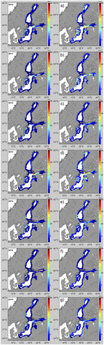
Year 2014 shows the highest frequency of upwelling in the southern part of the Bay of Bothnia reaching up to 20%. Similar values are observed on the west coast of the Baltic Sea and along Estonian coast. The phenomenon was also present along the Polish coast and in the Gulf of Riga, which is better represented in results from satellite measurements. Similarly to previous years, there are also many areas of less frequent events, under 10% of the time, visible along all Baltic coast. During 2015, upwelling occurred very often along the west coast of the Baltic Proper and along Finnish coast in the Gulf of Finland, up to 35% of the time, in the south of Gulf of Riga, ca. 25% along Polish coast, ca. 14%. Satellite data also show frequent upwelling in the northern part of the Bay of Bothnia, along Swedish coast. This is also the year in which differences between satellite and model data were most visible. After visual analysis of model data from this year, it was determined that very persistent upwelling events took place between second part of Jun and mid-August. For this time, there were very little data from satellite observations. In addition, some of upwellings were wrongly classified in satellite measurements as clouds. This led to a substantial difference between results obtained from these two sources. Similar spatial distribution of upwelling was observed for year 2016. However, the events along the Swedish coast in the Baltic Proper and in the Gulf of Finland were less frequent, ca. 26%, and there were more upwelling areas near the west coast of Bay of Bothnia. Satellite data also show more upwelling areas along the coasts of Poland, Lithuania and Latvia.

Upwelling frequencies for months from May to September

Spatial distribution of upwelling frequencies for each month from May to September calculated as average from years 2010–2016 have been analysed (Figure 6).

Figure 6. Monthly mean upwelling frequency distribution for May – September (a–e). Left – model, right – satellite.

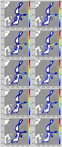
According to model results, during May the highest frequency of upwelling events was along Estonian coast, near Gulf of Riga's entrance and on the western part of the Polish coast, ca. 15%. Less frequent upwelling was observed along Gotland's west coast. Satellite data show much more events near entrance to Gulf of Riga and Gulf of Finland. However, after visual examination of SST data it was concluded that the upwelling detection in the aforementioned regions was erroneous. During June, frequency of upwelling events increased in most regions. In the Gulf of Finland, upwelling was observed for up to 30% of the time, in the Gulf of Riga and along east coast of Oland frequency of the event was up to 22% and along Polish coast and east coast of Baltic proper, up to 14%. Satellite data are in good correlation with model results, except for the Gulf of Riga's entrance, where much more frequent upwelling was shown. In July, a significant drop in the area covered by upwelling events was observed, especially in the Gulf of Finland, east and south coast of Baltic Proper. On the other hand, increase of frequencies of the phenomenon was observed along east coast of Baltic Proper, over 30% of the time, and along east coast of Bay of Bothnia, ca. 8%. Satellite data also showed upwelling events along Swedish coast in the northern part of the Bay of Bothnia, up to 30%. Similarly to July, during August, further decrease in upwelling area and frequency was observed in the Gulf of Finland and along east coast of Baltic Sea. There was also increase of upwelling frequencies and area along west coast and the south coast of Gotland, reaching up to 35%. In September, the event was rarely present in the east parts of the Baltic Sea, and its frequency along Swedish coast also decreased. This is inconsistent with satellite data that showed slight increase in upwelling area and frequency along Swedish coast. However, the presence of this event was much less visible in satellite data during August and this increase led, in fact, to better agreement between model and satellite results. Satellite results also showed upwelling areas along Polish coast with frequencies 15–22%, which are not visible in model results.

Wind

Table 1 presents the comparison of percentage of upwelling days derived from satellite and model data with percentage of days with favourable wind conditions described in ‘Methodology’ section. Numbers in first column correspond with locations from Figure 1. Following columns contain upwelling frequencies derived from satellite and model data and percentage of favourable days, respectively. One can see that percentage of upwelling days derived from model data is in good agreement with percentage of favourable wind conditions. Average difference is 2.64 pp., which corresponds to just 28 days during the 1071 days period. Highest differences, 6.9 and 6.4 pp., which correspond to ca. 70 days, were observed along Polish coast and in the Bay of Bothnia respectively, where the number of events was lower than expected. It was also much lower than that derived from satellite observations. In remaining six areas, the agreement between upwelling and wind is much better, and the difference does not exceed 3 pp., and in three cases it is under 1%.

Operational detection system

The operational module that manages upwelling detection system is implemented as an additional functionality to already working 3D CEMBS systems. The base system produces 48-h forecasts 4 times a day in approximately equal intervals. Forecasts temporal resolution is set to 1 h. Every time the main forecast calculations are completed system runs additional task that produces a map with a mask indicating if and where coastal upwelling was detected. This information is then stored in a binary file that is kept together with all the results of 3D CEMBS calculations. Results are presented online on the 3D CEMBS website www.cembs.pl. After choosing ‘UPWELLING’ from the menu user is redirected to upwelling detection tool homepage. This page provides a brief description of the method together with sample results and step-by-step instructions on how to generate upwelling map (Figures 7 and 8). Two clickable links redirect user to ‘FORECASTS’ and ‘ARCHIVE’ sections. This tool is enabled only between May and September following method's assumptions.

Figure 7. Upwelling Detection System website with an important navigation sections selected.

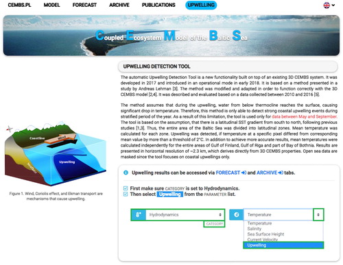
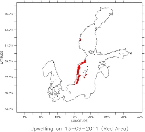
Figure 8. Sample map of places with an occurrence of upwelling on 18th August 2015 produced by the Upwelling Detection System.

Summary and discussion

Analysis conducted in this study allowed the assessment of frequency and locations of upwelling events in the Baltic Sea. It was shown that the phenomenon is most common along Swedish coast (up to 31%), along east coast of Oland (25–29%) and Gotland (ca. 20%) as well as in the Gulf of Finland (ca. 23%) and along Polish coast (up to 20%). It was found that results derived from NOAA/AVHRR satellite observations suggest higher number of upwelling days than those derived from 3D CEBMS model calculations. The highest difference was observed along the Polish coast (ca. 12 percentage points) and in the Gulf of Finland (ca. 7 percentage points). In the remaining areas, the difference was much lower and ranged between 0.8 and 5.4 pp. This corresponds to 8–58 days out of 1071 days period. This inconsistency was observed mainly very close to the coast, where satellite data showed highest frequencies of upwelling's presence. This feature was not visible in model data. It is caused mainly by model's boundary conditions stating that horizontal components of water velocity vector are set to zero in the grid cells adjacent to land. Another reason is model's vertical resolution. First four layers of model have thickness of 5 m. This can lead to differences between model results and actual conditions in shallow waters, close to the coast. There are a number of other factors, such as parameterisation of model equations responsible for wind stress, heat flux or vertical mixing. On the other hand, satellite measurements can also be prone to some errors. For example, Upwelling can be classified as a cloud and vice versa. Aside from aforementioned differences model and satellite data were in good agreement. Also changes in upwelling locations and intensity between consecutive years and months were moderately well preserved. Results of the analysis were also in good accordance with previous results (Lehmann et al. 2012). However, in some areas, e.g. along the Polish coast, where coastal upwelling is one of major factors affecting surface temperature distribution (Krężel et al. 2005) model results significantly underestimate the frequency of this event. Similar situation can be observed in Bay of Bothnia, where results derived from satellite data were more consistent. Analysis of statistics from Table 2 shows that the proposed method used with model data underestimates frequencies of upwelling events and is more likely to show false negative results than false positive. This means that it will rather miss an upwelling event than detect one when there is none. The accuracy of the method is very good, however, F1-score is much lower. TPR and PPV are in most cases close to each other, which means that the method is balanced between how many actual upwelling events were detected and how many detected events were actual upwellings. One can argue that with lower threshold for upwelling detection the method could give more detected instances of upwelling. However, this would also lead to more false detections. And whether more true positive or less false positive detections is better depends on the usage of the results. More appropriate way to improve the performance of this method is to further develop and improve the underlying model by e.g. increasing horizontal and vertical resolution, fine-tuning of parameterisation, etc.

Analysis of upwelling and wind series showed good correlation between these components. Highest differences between number of days with upwelling and favourable wind, ca. 6.5–7 pp. were found along Polish coast and in the Bay of Bothnia. This means that during the period of 1071 days upwelling was present 70 days less than the favourable winds. Remaining areas preserve very good correlation between these factors, with differences not exceeding 2.7 pp. This leads to a conclusion that assumptions made by Lehmann et al. (2012) about favourable wind conditions can be successfully applied for the analysis of 3D CEMBS results.

Time series analysed in this paper is too short to assess the presence of any trends in upwelling frequencies. Nonetheless, comparison with the results from previous studies shows further increase of upwelling frequencies along the Swedish coast and north Coast of the Gulf of Finland, as well as decrease in event incidence along east and Polish coast of the Baltic Sea. This suggests that the general trends are maintained. However, it should be kept in mind that datasets used for these two analyses came from different sources and were inconsistent, and the method of upwelling detection was slightly modified.

Acknowledgements

3D CEMBS model calculations presented in this paper were carried out on the Tryton supercomputer at the Academic Computer Centre (CI TASK) in Gdansk. This study has been conducted using Satellite Monitoring of the Baltic Sea Environment – SatBałtyk database. Partial support for this study was provided by the project ‘Integrated info-prediction Web Service WaterPUCK’ – no. BIOSTRATEG3/343927/3/NCBR/2017 and ‘Knowledge transfer platform FindFISH’ – no. RPPM.01.01.01-22-0025/16-00. The authors are grateful to the anonymous reviewers for valuable comments on earlier versions of the manuscript.

Disclosure statement

No potential conflict of interest was reported by the authors.

ORCID

Artur Nowicki http://orcid.org/0000-0003-3801-8137

Maciej Janecki http://orcid.org/0000-0002-8784-2862

Lidia Dzierzbicka-Głowacka http://orcid.org/0000-0001-6151-2390

Additional information

Funding

Partial support for this study was provided by the project ‘Integrated info-prediction Web Service WaterPUCK’ – no. BIOSTRATEG3/343927/3/NCBR/2017 and ‘Knowledge transfer platform FindFISH’ – no. RPPM.01.01.01-22-0025/16-00.

References

- Bychkova I, Viktorov S, Shumakher D. 1988. A relationship between the large-scale atmospheric circulation and the origin of coastal upwelling in the Baltic. Meteorol Gidrol. 10:91–98.
- Chaudhari S, Balasubramanian R, Gangopadhyay A. 2008. Upwelling detection in AVHRR sea surface temperature (SST) images using neural-network framework. Proc IEEE Int Geosci Remote Sens Symp. 2:926–929.
- Darecki M, Ficek D, Krężel A, Ostrowska M, Majchrowski R, Woźniak SB, Bradtke K, Dera J, Woźniak B. 2008. Algorithm for the remote sensing of the Baltic ecosystem (DESAMBEM). Part 2: empirical validation. Oceanologia. 50(4):509–538.
- Dzierzbicka-Głowacka L, Jakacki J, Janecki M, Nowicki A. 2013a. Activation of the operational ecohydrodynamic model (3D CEMBS) – the hydrodynamic part. Oceanologia. 55(3):519–541. doi: 10.5697/oc.55-3.519
- Dzierzbicka-Głowacka L, Janecki M, Nowicki A, Jakacki J. 2013b. Activation of the operational ecohydrodynamic model (3D CEMBS) – the ecosystem module. Oceanologia. 55(3):543–572. doi: 10.5697/oc.55-3.543
- Dzierzbicka-Głowacka L, Nowicki A, Janecki M. 2013c. The automatic monitoring system for 3D-CEMBSv2 in the operational version. J Environ Sci Eng Technol. 1:1–9. doi: 10.12974/2311-8741.2013.01.01.1
- Fennel W, Seifert T, Kayser B. 1991. Rossby radii and phase speeds in the Baltic Sea. Cont Shelf Res. 11(1):23–36. doi: 10.1016/0278-4343(91)90032-2
- Gidhagen L. 1987. Coastal upwelling in the Baltic Sea—satellite and in situ measurements of sea-surface temperatures indicating coastal upwelling. Estuar Coast Shelf Sci. 24(4):449–462. doi: 10.1016/0272-7714(87)90127-2
- Herman-Iżycki L, Jakubiak B, Nowiński K, Niezgódka B. 2002. UMPL – the numerical weather prediction system for operational Applications. In: Research works based on the ICMs UMPL numerical weather prediction system results. Warsaw: ICM Publishing; p. 14–27.
- Jankowski A. 2002. Variability of coastal water hydrodynamics in the southern Baltic – hindcast modelling of an upwelling event along the Polish coast. Oceanologia. 44(4):395–418.
- Krężel A, Ostrowski M, Szymelfenig M. 2005. Sea surface temperature distribution during upwelling along the Polish Baltic coast. Oceanologia. 47(4):415–432.
- Lehmann A, Myrberg K. 2008. Upwelling in the Baltic Sea – a review. J Mar Syst. 74 Supplement: S3-S12, Baltic Sea Science Congress 2007.
- Lehmann A, Myrberg K, Höflich K. 2012. A statistical approach to coastal upwelling in the Baltic Sea based on the analysis of satellite data for 1990–2009. Oceanologia. 54(3):369–393. doi: 10.5697/oc.54-3.369
- Li X, Dmith DK, Keiser K. 2012. Method for detecting wind and cold water upwelling events from satellite data. Proceedings 92 American Meteorological Society Annual Meeting. New Orleans, LA. American Meteorological Society.
- Marcello J, Marques F, Eugenio F. 2005. Automatic tool for the precise detection of upwelling and filaments in remote sensing imagery. IEEE Trans Geosci Remote Sens. 43(7):1605–1616. doi: 10.1109/TGRS.2005.848409
- Myrberg K, Andrejev O. 2003. Main upwelling regions in the Baltic Sea - a statistical analysis based on three-dimensional modelling. Boreal Environ Res. 8:97–112.
- Nascimento S, Franco P, Sousa F, Dias J, Neves F. 2012. Automated computational delimitation of SST upwelling areas using fuzzy clustering. Comput Geosci. 43:207–216. doi: 10.1016/j.cageo.2011.10.025
- Nowicki A, Dzierzbicka-Głowacka L, Janecki M, Kałas M. 2015. Assimilation of the satellite SST data in the 3D CEMBS model. Oceanologia. 57(1):17–24. doi: 10.1016/j.oceano.2014.07.001
- Osiński R, Rak D, Walczowski W, Piechura J. 2010. Baroclinic Rossby radius of deformation in the southern Baltic Sea. Oceanologia. 52(3):417–429. doi: 10.5697/oc.52-3.417
- Ostrowska M, Darecki M, Kowalewski M, Krężel A, Dera J. 2015. System SatBałtyk - satelitarny monitoring środowiska Bałtyku. Struktura, funkcjonowanie, możliwości operacyjne, 1st ed. Sopot: Institute of Oceanology, Polish Academy of Sciences. Polish.
- Plattner S, Mason DM, Leshkevich GA, Schwab DJ, Rutherford ES. 2006. Classifying and forecasting coastal upwelling in lage mishigan using satellite derived temperature images and buoy data. J Gt Lakes Res. 32(1):63–76. doi: 10.3394/0380-1330(2006)32[63:CAFCUI]2.0.CO;2
- Tamin A, Minaoui K, Daoudi K, Atillah A, Yahia H, Aboutajdine D. 2014. Upwelling detection in SST images using fuzzy clustering with adaptive cluster merging. Marrakech, Morocco: The eighth edition of International Symposium on signal, Image, Video and Communications (ISIVC).
- Voipio A. 1981. The Baltic Sea. 1st ed. Vol. 30. Helsinki, Finland: Elsevier Scientific Publishing.
- Woźniak B, Krężel A, Darecki M, Woźniak SB, Majchrowski R, Ostrowska M, Kozłowski Ł, Ficek D, Olszewski J, Dera J. 2008. Algorithm for the remote sensing of the Baltic ecosystem (DESAMBEM). part 1: Mathematical apparatus. Oceanologia. 50(4):451–508.