Extrapolating Eulerian ocean currents for improving surface drift forecasts

ABSTRACT

Predictions of drift trajectories based on four drift models were compared with observations from drifting buoys deployed in 2014 and 2015 in the Estuary and Gulf of St. Lawrence to show the impact of the current vertical shear on the surface drift predictions. Input of ocean currents and winds are obtained from ISMER's 5 km resolution ocean circulation model and from the Canadian Regional Deterministic Prediction System, respectively. The control drift model A considers depth-averaged near-surface currents (0–5 m) provided by the top grid cell of the ocean circulation model. Model B performs a linear extrapolation assuming a constant vertical shear equal to that between the first two cells of the ocean model. Models C and D perform a dynamic extrapolation assuming an Ekman layer with a constant or linearly increasing vertical viscosity, respectively. Model performance is evaluated based on several error metrics. Drift models based on extrapolated surface currents reduce separation distances relative to the control model by 25% (model B), 31% (model C) and 35% (model D) on average, for lead times from 3 h to 72 h. We thus recommend the use of extrapolation methods of near-surface ocean currents for improving surface drift forecasting skills in support of emergency response.

KEYWORDS:

• Surface drift forecast
• Ekman layer
• drifting buoys
• shear extrapolation

1. Introduction

Lagrangian drift forecasts are essential for planning search and rescue operations at sea (Hackett et al. 2006; Breivik and Allen 2008; Davidson et al. 2009; Breivik et al. 2011; Breivik et al. 2013) and for effective and rapid intervention in case of oil spills (Eide et al. 2007; Broström et al. 2011; Paris et al. 2012; Maßmann et al. 2014; Jones et al. 2016). They are also useful for identifying priority intervention zones and for evaluating potential environmental impacts associated with pollution events (Bourgault et al. 2014).

Lagrangian transport models have extensively been used to study ecological and evolutionary connectivity among marine populations (Henry et al. 2018; Lequeux et al. 2018). They are used to locate fish larvae recruitment zones (Daewel et al. 2015) and their connectivity with coral reef organisms (Mayorga–Adame et al. 2017), to evaluate stocks (Röhrs et al. 2014), to assess the risk associated to invasive species (Brandt et al. 2008) and toxic algal blooms (Masó et al. 2003; Havens et al. 2010), including in the St. Lawrence Estuary (Starr et al. 2017), to track suspended microplastics in the marine environment (Van Sebille et al. 2012, 2015) and to determine the origin and formation of water masses (Soomere et al. 2010), using a large number of trajectories (Döös 1995; Blanke and Raynaud 1997; Döös et al. 2004).

The drift of a floating object is driven by the drag force imposed by the flow of water around it, that we call ${\mathit{u}}_O$, and in the case where it has an emerged part, by the drag imposed by the flow of air on this part, which we call ${\mathit{u}}_A$. If those two vector quantities were known, neglecting acceleration, the drift velocity ${\mathit{u}}_{\mathrm{d}}$ of the object would be obtained as(1) ${\mathit{u}}_{\mathrm{d}}={\mathit{u}}_O+\tilde{\alpha }{\mathit{u}}_A$(1) where $\tilde{\alpha }$ is obtained by balancing the air and water drag forces acting simultaneously on the object, usually defined as the Nansen Number $\mathrm{N}\mathrm{a}=\sqrt{{\rho }_a{C}_a/{\rho }_w{C}_w}$, with ${\rho }_a$ and ${\rho }_w$ the air and seawater densities, and $C_a$ and $C_w$ the air and water drag coefficients (Leppäranta 2011). However, the terms on the right-hand side of Equation (1(1) ${\mathit{u}}_{\mathrm{d}}={\mathit{u}}_O+\tilde{\alpha }{\mathit{u}}_A$(1) ) depend on a number of nonlinear physical processes happening in the atmosphere-ocean boundary layer that must be parameterised from fields produced by operational forecasting systems. One approach commonly adopted is to assume that the drift is a linear combination of velocity terms each related to a given process. Following De Dominicis et al. (2014) as an example approach, the drift velocity is estimated by(2) ${\mathit{u}}_{\mathrm{d}}={\mathit{u}}_E+{\mathit{u}}_S+{\mathit{u}}_W+{\mathit{u}}_D+{\mathit{u}}^{\mathrm{\prime }}$(2) where ${\mathit{u}}_E$ is the Eulerian current, ${\mathit{u}}_S$ is the wave-induced Stokes drift, ${\mathit{u}}_W$ is the local wind velocity correction term, ${\mathit{u}}_D$ is a correction term due to wind drag on the emerged part of the floating object called windage (De Dominicis et al. 2014). These four terms form the deterministic model that we wish to be as accurate as possible. The last term ${\mathit{u}}^{\mathrm{\prime }}$ is a randomly fluctuating velocity accounting for the dispersion due to unresolved physical processes and model errors. Parameterisations of the deterministic terms are based on outputs obtained from ocean, atmosphere and wave models. The Eulerian current velocity is taken from the first (top) cell of an ocean circulation model, that we here call ${\mathit{u}}_{E1}$, the wind velocity at 10 m above the sea surface ${\mathit{U}}_{10}$ is obtained from an atmospheric model, and the Stokes drift ${\mathit{u}}_S$ is obtained from a spectral wave model. Figure 1 is a schematic showing the three velocity fields that are available and used to estimate the drift ${\mathit{u}}_{\mathrm{d}}$ of a floating object. When the wave-induced drift is not explicitly taken into account, as it is the case for the operational drift forecast system in Canada, the deterministic drift model deriving from Equation (2(2) ${\mathit{u}}_{\mathrm{d}}={\mathit{u}}_E+{\mathit{u}}_S+{\mathit{u}}_W+{\mathit{u}}_D+{\mathit{u}}^{\mathrm{\prime }}$(2) ) is given by the following, widely-used equation (Al–Rabeh 1994; Hackett et al. 2006; Breivik and Allen 2008; Callies et al. 2017)(3) ${\mathit{u}}_{\mathrm{d}}={\mathit{u}}_{E1}+\alpha {\mathit{U}}_{10}$(3) where $\alpha$ is a parameter that is determined empirically based on observations and tuned for specific applications. This model thus assumes that the drift of a floating object is the ocean current velocity to which a wind correction term is added. This correction term implicitly and simultaneously accounts for windage, for the wave-induced contribution as well as the unresolved wind-dependent vertical shear of the Eulerian current. While $\alpha$ is assumed real (i.e. the result of a linear regression between scalar quantities) it can also be obtained from a complex linear regression between the observed drift velocity vectors, to which the predicted ocean current is subtracted, and wind velocity vectors. This allows applying a correction that could be rotated with respect to wind direction. The modulus of α is in the order of a few percent. Although it is typically the same order of magnitude as the Nansen number Na defined earlier, it must be remembered that it represents more than just the effect of the direct wind drag on the object. We thus call $\alpha {\mathit{U}}_{10}$ a wind correction term, as in De Dominicis et al. (2014), instead of windage.

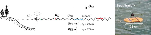
Figure 1. A schematic of the surface drift problem in a fetch-limited environment. A floating object drifts at the ocean's surface at a velocity ${\mathit{u}}_{\mathrm{d}}$ (green arrow), which is estimated using the mean Eulerian current ${\mathit{u}}_E$, the wind velocity ${\mathit{U}}_{10}$, and the Lagrangian Stokes drift ${\mathit{u}}_S$ (red arrows). The Eulerian current velocity ${\mathit{u}}_E$ is vertically sheared and is provided by a numerical ocean circulation model at the centre of vertical grid cells ${\mathit{u}}_E\left(z_1\right)={\mathit{u}}_{E1}$ and ${\mathit{u}}_E\left(z_2\right)={\mathit{u}}_{E2}$. The surface current velocity (${\mathit{u}}_{E0}$, blue arrow) is obtained by extrapolation methods. To the right is a picture of a drifting buoy designed and built at Institut des sciences de la mer de Rimouski floating in the St. Lawrence Estuary. The Spot Trace${}^{\mathrm{T}\mathrm{M}}$ device is attached to the 33 cm-wide and 4 cm-thick wooden platform with a springing metal coil.

In this paper, we focus our attention on the wind-induced vertical shear that is often unresolved in the first 1 or 2 metres by ocean circulation models and that is implicitly included in the wind correction term of Equation (3(3) ${\mathit{u}}_{\mathrm{d}}={\mathit{u}}_{E1}+\alpha {\mathit{U}}_{10}$(3) ). A number of studies (Gästgifvars et al. 2006; De Dominicis et al. 2012; Kjellsson and Döös 2012) concluded or suggested that surface currents taken from ocean circulation models were too small compared to the surface drift. Callies et al. (2017) showed that by increasing the vertical resolution of an ocean circulation model from 5 m to 1 m significantly increased the performance of surface drift predictions while decreasing the relative importance of the wind correction term ($\left|\alpha \right|\to 0$). This suggests that most operational ocean forecasting systems do not sufficiently resolve the vertical shear near the surface. For example, the surface current provided by the Canadian Atmosphere-Ocean-Ice forecast system for the Gulf of St. Lawrence (Smith et al. 2012) is given at the centre of the top grid cell (0–5 m), which is a typical value in many operational systems. Since the relationship between the surface current and the current at a certain depth (e.g. at $z$ = 2.5 m) is not linear, the linear wind correction term cannot completely account for the unresolved vertical shear, which may decrease the correlation between the observed and simulated drift velocities (see Figure 1). The current magnitude can decrease rapidly immediately below the surface, even over the first few millimetres (Fernandez et al. 1996), and its direction can change due to Ekman dynamics (Ekman 1905). The results of Callies et al. (2017) also imply that the wind correction term accounts predominantly for the unresolved near-surface vertical shear.

Considering this, improving operational drift forecast systems would imply increasing model's vertical resolution. Such a strategy can be very difficult and arduous due to practical reasons such as significant increases in computational costs, extensive model development, calibration and verification, etc. In this paper, we implement and test two methods that extrapolate the current velocity provided by a regional ocean circulation model for Estuary and the Gulf of St. Lawrence (EGSL), Canada, to the surface, and we assess how these methods improve surface drift forecasts. Our main goal is to reduce the bias in the standard drift model based on drift current of Equation (3(3) ${\mathit{u}}_{\mathrm{d}}={\mathit{u}}_{E1}+\alpha {\mathit{U}}_{10}$(3) ) which is used in operational drift forecast applications. Many studies compared simulated with observed trajectories to validate drift model performance (Al–Rabeh 1994, 2000; Price et al. 2006; Barron et al. 2007; Caballero et al. 2008; Huntley et al. 2011; Cucco et al. 2012; Ivichev et al. 2012; Röhrs et al. 2012; De Dominicis et al. 2013, 2014; Callies et al. 2017). Here we adopt a similar methodology by using data obtained from a large number of drifting buoys in the EGSL, to evaluate the drift model performance based on Lagrangian trajectory evaluation metrics. The drifters and the extrapolation methods are described in Section 2. Section 3 presents the results that are discussed in Section 4.

2. Methods

2.1. Drifters

Drifting buoys were built and designed at Institut des sciences de la mer de Rimouski (ISMER). They consist in a 4 cm-thick plate of 25–40 cm in diameter made of pine wood studs fixed together with aluminium bars (Figure 1). A GPS tracking device (Spot Trace${}^{\mathrm{T}\mathrm{M}}$) is fixed to the plate with a loosened spring in order to maintain the device in a state of motion that prevents entering the quiet mode during which the device does not transmit its position. It is programmed to send its location every 10 minutes during the tracking mode. A weight of 1 kg is attached to the plate with a nylon wire and hangs 20–30 cm below the plate to avoid capsizing in wavy conditions. ISMER's buoys are meant to be comparable to small debris floating near the surface with a minimum windage.

Deployments were conducted in the southeastern portion of the Gulf of St. Lawrence, in the vicinity of the Old Harry prospect site (Bourgault et al. 2014) in June–July and October–November 2014, in Baie des Chaleurs in June–July 2015, and in the Lower St. Lawrence Estuary in August–September 2014 and 2015. A total of 40 trajectories 1 to 35-day long produced 61,169 displacement data points in the EGSL from 2014 to 2015 (Figure 2(a)). The average displacement is 33.5 km per day. In our analysis, we only considered displacements calculated from consecutive data points recorded less than one hour apart, and located within the ocean model domain (see Section 2.2), giving a total of 58,612 data points.

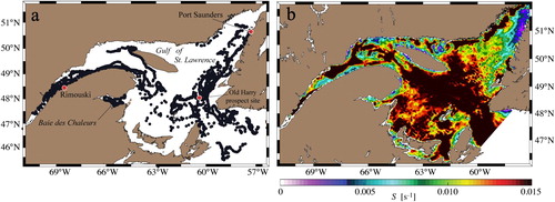
Figure 2. (a) Geographical positions reported by drifting buoys between 2014 and 2015 (61,169 points) in the Lower Estuary, near Rimouski, in Baie des Chaleurs, and around the Old Harry Prospect site. (b) Daily averaged vertical shear magnitude $S$ in s${}^{-1}$ calculated using the two top cells of the GSL5km-RDPS model for 2 June 2014.

2.2. Winds and near-surface Eulerian currents

Hourly wind vectors ${\mathit{U}}_{10}$ are obtained from a 35-km resolution limited-area configuration of the Regional Deterministic Prediction System (RDPS) atmospheric model centred over the EGSL, that is operated by Environment and Climate Change Canada (ECCC) for weather prediction (Smith et al. 2012). Eulerian ocean currents are obtained from a 5-km resolution coupled ice-ocean circulation model over the Gulf of St. Lawrence (GSL5km). The ocean component is a hydrostatic, Boussinesq primitive equation model that is driven by tides propagating from the Atlantic Ocean through two open boundaries. Friction and diffusion are solved by a turbulent kinetic energy equation with a Mellor-Yamada level 2.5 closure (Mellor and Yamada 1974). Freshwater river runoffs are prescribed as boundary conditions on momentum and salinity, interpolated in time from observations in the 28 most important tributaries (HYDAT database, Environment and Climate Change Canada), normalised to represent the input from the neighbouring drainage basins. The St. Lawrence River runoff is taken from the monthly reanalysis of (Bourgault and Koutitonsky 1999). This model reproduces the main features of the estuarine circulation, water masses distribution and their seasonal variability. It is worth noting that buoys were deployed in locations with contrasted stratification and fetch conditions, from the narrow maritime estuary to the open outer gulf regions. The interested reader will find further details about this model as well as informative figures about this coastal system in Saucier et al. (2003).

The GSL5km was forced by the RDPS atmospheric fields (hereafter referred to as GSL5km-RDPS) during the period 1997–2015 and provided ocean currents every hour. The ocean vertical grid has a 5 m resolution from the surface down to a depth of 300 m, and 10 m from 300 m to the bottom. Horizontal currents are computed at the centre of the vertical cells. The current velocity values for the top two first cells of the water column, ${\mathit{u}}_{E1}$ and ${\mathit{u}}_{E2}$, are given at $z_1=2.5$ m and $z_2=7.5$ m, respectively (see Figure 1), with the $z$-axis oriented positive downward, unless otherwise specified. Ocean vertical and horizontal physics being computed with finite difference schemes, the vertical profile of current velocities is assumed linear between cells. In the presence of a vertical shear of horizontal currents, which is the case in wind-driven conditions, the current velocity values in the top cell may underestimate the surface current. The right panel of Figure 2 shows the daily-averaged vertical shear, computed as $S=\left|\right({\mathit{u}}_{E2}-{\mathit{u}}_{E1}\left)\right|/(z_2-z_1)$, for the 2 June 2014. Values reach up to $2.3\times {10}^{-2}$ s${}^{-1}$, even though the colour scale saturates at $1.5\times {10}^{-2}$ s${}^{-1}$, suggesting that ${\mathit{u}}_{E1}$ significantly underestimate the surface current. Extrapolating the currents to the surface is the purpose of the methods presented in the next section.

2.3. Extrapolation methods

In this section we describe two methods to extrapolate currents at the surface (z = 0) taking into account information about the vertical shear. The drift models we propose here follow the form of Equation (3(3) ${\mathit{u}}_{\mathrm{d}}={\mathit{u}}_{E1}+\alpha {\mathit{U}}_{10}$(3) ) in which we modify the expression for the Eulerian current and α. In the following, we will present four models that we label A, B, C and D to which correspond an Eulerian current velocity and a wind-correction coefficient $\alpha$ (see Table 1). Model A represents the control model using the current of the top cell of the GSL5km-RDPS model ${\mathit{u}}_{E1}$ and ${\alpha }_{\mathrm{A}}$.

Table 1. Wind correction coefficient α and drift model performances according to the metrics described in Section 2.5. Bold values represent best performances. Tolerances represent standard deviations for 1000 bootstrap resamples.

		Model A	Model B	Model C	Model D
$\alpha$		0.023 ${\mathrm{e}}^{i0.87}$	0.018 ${\mathrm{e}}^{i0.02}$	0.016 ${\mathrm{e}}^{i0.02}$	0.013 ${\mathrm{e}}^{i0.008}$
Metric	Lead time
RMSE (m s^−1)		0.17 ± 0.02	0.15 ± 0.02	0.16 ± 0.02	0.15 ± 0.02
r = |r| ${\mathrm{e}}^{i\theta }$		0.61 ${\mathrm{e}}^{-i0.14}$	0.69 ${\mathrm{e}}^{-i0.11}$	0.73 ${\mathrm{e}}^{i0.10}$	0.77 ${\mathrm{e}}^{i0.08}$
${⟨\phi ⟩}_i$ (${}^{\circ }$)		−3.2 ± 57.5	−2.1 ± 45.5	1.9 ± 44.3	1.3 ± 42.5
$d{s}_i$ (km)
	3 h	1.5 ± 0.8	1.1 ± 0.8	1.0 ± 0.7	0.8 ± 0.5
	6 h	2.8 ± 1.5	2.1 ± 1.1	1.8 ± 1.1	1.7 ± 0.8
	12 h	5.8 ± 2.5	4.3 ± 2.0	4.0 ± 1.5	3.8 ± 1.5
	24 h	9.0 ± 5.0	7.3 ± 3.0	6.3 ± 2.0	5.7 ± 1.8
	48 h	15 ± 10	12 ± 8	11 ± 7	10 ± 6
	72 h	21 ± 16	17 ± 13	16 ± 13	16 ± 12
ssc
	3 h	0.70 ± 0.09	0.78 ± 0.06	0.85 ± 0.05	0.89 ± 0.07
	6 h	0.66 ± 0.08	0.74 ± 0.05	0.81 ± 0.05	0.86 ± 0.05
	12 h	0.65 ± 0.07	0.75 ± 0.06	0.86 ± 0.06	0.87 ± 0.06
	24 h	0.63 ± 0.12	0.78 ± 0.08	0.83 ± 0.07	0.84 ± 0.07
	48 h	0.62 ± 0.16	0.75 ± 0.12	0.79 ± 0.11	0.83 ± 0.11
	72 h	0.61 ± 0.29	0.73 ± 0.17	0.76 ± 0.17	0.79 ± 0.17
ΔAi (%)
	3 h	–	28 ± 3	35 ± 2	41 ± 2
	6 h	–	26 ± 3	34 ± 3	38 ± 2
	12 h	–	27 ± 3	32 ± 2	33 ± 2
	24 h	–	26 ± 3	31 ± 3	35 ± 3
	48 h	–	22 ± 4	30 ± 3	33 ± 3
	72 h	–	20 ± 5	23 ± 4	34 ± 4

The first method we propose to estimate the surface current is a linear extrapolation of the velocities in the two top cells of the ocean circulation model, which corresponds to model B given by(4) ${\mathit{u}}_{E0}^{\mathrm{B}}=\frac{z_2{\mathit{u}}_{E1}-z_1{\mathit{u}}_{E2}}{z_2-z_1}$(4) where ${\mathit{u}}_{E1}$ and ${\mathit{u}}_{E2}$ are defined in Section 2.2 and are obtained from the GSL5km-RDPS model simulation at a hourly frequency. This method assumes that the vertical shear between $z_1$ and $z_2$ is the same as between the surface ($z_0=0$) and $z_1$.

The second method assumes that the horizontal velocity profile is the result of the Ekman balance in the upper ocean in response to a time-varying wind forcing. For this we follow the method of Elipot and Gille (2009) who estimate near-surface ageostrophic velocity at a given depth in the spectral domain as a convolution of the wind stress with the impulse response function. For a horizontally homogeneous oceanic boundary layer, neglecting horizontal gradients and pressure, we recall the linearised horizontal momentum balance to be (Price and Sundermeyer 1999; Elipot and Gille 2009)(5) $\frac{\mathrm{\partial }\mathit{u}(t,z)}{\mathrm{\partial }t}+if\mathit{u}(t,z)=\frac{\mathrm{\partial }}{\mathrm{\partial }z}\left[K_z\frac{\mathrm{\partial }\mathit{u}(t,z)}{\mathrm{\partial }z}\right]$(5) where the vector current is expressed in complex form $\mathit{u}=u+iv$, the second term is the horizontal component of the Coriolis acceleration with f the Coriolis parameter, and $K_z$ is the turbulent viscosity. The boundary condition at the surface of the ocean is(6) $K_z{\left.\frac{\mathrm{\partial }\mathit{u}}{\mathrm{\partial }z}\right|}_{z=0}=\frac{\mathit{\tau }}{\rho }$(6) where ρ is the seawater density and $\mathit{\tau }$ the wind stress. A velocity vector times series $\mathit{u}$ can be represented as a complex Fourier series of oscillating terms with a fundamental period T such that(7) $\mathit{u}\left(t\right)=u\left(t\right)+iv\left(t\right)=\sum _{k=-\mathrm{\infty }}^{+\mathrm{\infty }}{\mathit{U}}_k{\mathrm{e}}^{2i\pi {\nu }_{k}t}$(7) where ${\nu }_k=k/T$ are the discrete frequencies and ${\mathit{U}}_k$ are the complex Fourier coefficients given as(8) ${\mathit{U}}_k=\frac{1}{T}{\int }_0^T\mathit{u}\left(t\right){\mathrm{e}}^{-2i\pi {\nu }_{k}t}\mathrm{d}t$(8) The observed and theoretical ocean response to wind forcing strongly depends on the time scale (Elipot and Gille 2009). Taking into account temporal variations of the wind stress, the variation of the current $\mathit{u}(t,z)$ as a function of time and depth can be obtained from the convolution of the wind stress with the impulse response function $\mathit{h}(t^{\prime },z)$ where $t^{\prime }$ is the time lag (Broche et al. 1983; Elipot and Gille 2009)(9) $\mathit{u}(t,z)={\int }_0^{\mathrm{\infty }}\mathit{h}(t^{\prime },z)\tau (t-t^{\prime })\mathrm{d}{t}^{\prime }$(9) Taking the Fourier transform of Equation (9(9) $\mathit{u}(t,z)={\int }_0^{\mathrm{\infty }}\mathit{h}(t^{\prime },z)\tau (t-t^{\prime })\mathrm{d}{t}^{\prime }$(9) ) and using the convolution theorem, we obtain a linear relationship in the Fourier space between the wind stress and a transfer function(10) $\mathit{U}(\nu ,z)=\mathit{H}(\nu ,z)\mathit{T}\left(\nu \right)$(10) where $\mathit{U}$, $\mathit{H}$ and $\mathit{T}$ are the Fourier transforms of $\mathit{u}$, $\mathit{h}$ and $\mathit{\tau }$, respectively. At any frequency $\nu$, the transfer function $\mathit{H}$ is complex valued. Equation (10(10) $\mathit{U}(\nu ,z)=\mathit{H}(\nu ,z)\mathit{T}\left(\nu \right)$(10) ) shows that it's possible to compute the current at all depths from a given wind stress time series knowing the transfer function $\mathit{H}$ (Gonella 1972; Weller 1981; Rudnick and Weller 1993; Elipot and Gille 2009). Alternatively, we will use the transfer function $\mathit{H}$ to obtain the current at the surface based on the current known at a depth $z_1=2.5$ m provided by the GSL5km-RDPS model.

Because the transfer function $\mathit{H}$ only accounts for wind-driven dynamics, surface currents resulting from Equation (10(10) $\mathit{U}(\nu ,z)=\mathit{H}(\nu ,z)\mathit{T}\left(\nu \right)$(10) ) represent the ageostrophic wind-driven current. We thus extract the surface geostrophic current ${\mathit{u}}_{\mathrm{g}}(z_0,t)$ (neglecting the vertical geostrophic shear between $z_0$ and $z_1$) and tidal current ${\mathit{u}}_{\mathrm{t}\mathrm{i}\mathrm{d}\mathrm{e}}(z_1,t)$ from the total current provided by the GSL5km-RDPS model to obtain the ageostrophic current ${\mathit{u}}_{\mathrm{a}\mathrm{g}}(z_1,t)$:(11) ${\mathit{u}}_{\mathrm{a}\mathrm{g}}(z_1,t)=\mathit{u}(z_1,t)-{\mathit{u}}_{\mathrm{g}}(z_0,t)-{\mathit{u}}_{\mathrm{t}\mathrm{i}\mathrm{d}\mathrm{e}}(z_1,t).$(11) The tidal current ${\mathit{u}}_{\mathrm{t}\mathrm{i}\mathrm{d}\mathrm{e}}(z_1,t)$ is computed using the Matlab T-Tide harmonic analysis toolbox (Pawlowicz et al. 2002), while the surface geostrophic current is computed using the sea surface height η from the GSL5km-RDPS model using(12) ${\mathit{u}}_{\mathrm{g}}(z_0,t)=\mathit{k}\times \frac{g}{f}\mathrm{\nabla }\eta .$(12) η is detided and low-pass filtered with a cutoff period $T_c=17$ h, corresponding to the local inertial frequency.

Next, we compute the Fourier transform of ${\mathit{u}}_{\mathrm{a}\mathrm{g}}$ at $z_0=0$ m using its known values at $z_1$ and Equation (10(10) $\mathit{U}(\nu ,z)=\mathit{H}(\nu ,z)\mathit{T}\left(\nu \right)$(10) )(13) ${\mathit{U}}_{\mathrm{a}\mathrm{g}}(z_0,\nu )=\frac{\mathit{H}(z_0,\nu )}{\mathit{H}(z_1,\nu )}{\mathit{U}}_{\mathrm{a}\mathrm{g}}(z_1,\nu ),$(13) The surface velocity ${\mathit{u}}_{\mathrm{a}\mathrm{g}}(z_0,t)$ is then obtained by applying the inverse Fourier transform(14) ${\mathit{u}}_{\mathrm{a}\mathrm{g}}(z_0,t)={\int }_{-\mathrm{\infty }}^{+\mathrm{\infty }}\frac{\mathit{H}(z_0,\nu )}{\mathit{H}(z_1,\nu )}{\mathit{U}}_{\mathrm{a}\mathrm{g}}(z_1,\nu ){\mathrm{e}}^{2i\pi \nu t}\mathrm{d}\nu .$(14) Finally, the total surface current is retrieved as(15) $\mathit{u}(z_0,t)={\mathit{u}}_{\mathrm{a}\mathrm{g}}(z_0,t)+{\mathit{u}}_{\mathrm{g}}(z_0,t)+{\mathit{u}}_{\mathrm{t}\mathrm{i}\mathrm{d}\mathrm{e}}(z_1,t),$(15) neglecting the vertical shear of tidal currents between $z_0$ and $z_1$. The transfer function $\mathit{H}$ is determined by solving the following ordinary differential equation for $\mathit{U}(\nu ,z)$, obtained by applying the Fourier transform to Equation (5(5) $\frac{\mathrm{\partial }\mathit{u}(t,z)}{\mathrm{\partial }t}+if\mathit{u}(t,z)=\frac{\mathrm{\partial }}{\mathrm{\partial }z}\left[K_z\frac{\mathrm{\partial }\mathit{u}(t,z)}{\mathrm{\partial }z}\right]$(5) ) (Elipot and Gille 2009)(16) $i(2\pi \nu +f)\mathit{U}(z,\nu )-\frac{d}{dz}\left[K_z\left(z\right)\frac{d\mathit{U}(z,\nu )}{dz}\right]=0.$(16) The specific form of $\mathit{H}$ will depend on how we choose the boundary conditions and $K_z\left(z\right)$. Among the nine models considered by Elipot and Gille (2009) (their Figure 1), we rejected those with infinite velocity at the surface as well as those with a vanishing velocity at the base of the finite boundary layer. In the four remaining models, two required a finite boundary layer depth to be determined. Although we tested them all, here we present only the two models that provide the best results while remaining simple (i.e. a smaller number of tuning parameters). The chosen transfer functions both assume a homogeneous ocean of infinite depth, but with two different vertical viscosity profiles that are shown in Figure 3(b). The bottom boundary condition is chosen so that $\mathit{u}(t,z)$ and $\mathit{U}(\nu ,z)$ tend to 0 as $z\to +\mathrm{\infty }$.

Figure 3. (a) Magnitude of average near-surface horizontal current profiles produced by extrapolating the Eulerian current ${\mathit{u}}_{E1}$ from the GSL5km model with drift models B (${\mathit{u}}_E^{\mathrm{B}}$, brown), C (${\mathit{u}}_E^{\mathrm{C}}$, light blue) and D (${\mathit{u}}_E^{\mathrm{D}}$, dark blue). The currents are averaged over all observed drifter locations. (b) Profiles of turbulent diffusivity $K_z\left(z\right)$ used in drift models C (solid) and D (dash).

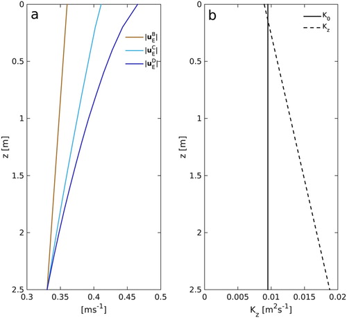
The transfer function that we consider for model C is the one obtained with a constant viscosity profile $K_0$, which is taken from Table 1 of Elipot and Gille (2009):(17) ${\mathit{H}}_{\mathrm{C}}(\nu ,z)=\frac{{\mathrm{e}}^{-i\pi /4}{\mathrm{e}}^{-z(1+i)/{\delta }_1}}{\rho \sqrt{(2\pi \nu +f)K_0}}$(17) with(18) ${\delta }_1=\sqrt{2K_0/(2\pi \nu +f)}.$(18) The diffusivity value is given by $K_0=d^{2}f/2$ (Ekman 1905; Chereskin 1995) where $d$ is the traditional Ekman depth defined as(19) $d={\delta }_1(\nu =0)=\frac{z_2-z_1}{\ln \left[⟨\frac{\left|{\mathit{u}}_{\mathrm{a}\mathrm{g}}\left(z_2\right)\right|}{\left|{\mathit{u}}_{\mathrm{a}\mathrm{g}}\left(z_1\right)\right|}⟩\right]}$(19) where angle brackets correspond to temporal averaging.

The second transfer function that we consider for model D assumes a viscosity that is finite at the surface and increases linearly with depth (Figure 3(b)) as(20) $K\left(z\right)=K_1(z_{\ast }+z)$(20) where $K_1=\kappa u_{\ast }$ (Lewis and Belcher 2004), $\kappa =0.4$ is von Karman's constant and $u_{\ast }=\sqrt{\tau /\rho }$ is the ocean friction velocity associated with the surface wind stress. The roughness length $z_{\ast }$ is parameterised as in Lewis and Belcher (2004) to account for vertical mixing induced by surface gravity waves. It is expressed by(21) $z_{\ast }=\frac{\kappa u_{\ast a}}{4f}\sqrt{\frac{{\rho }_a}{\rho }}\exp \left[-q\kappa \sqrt{\frac{\rho }{{\rho }_a}}\frac{\left|{\mathit{U}}_{10}\right|}{u_{\ast a}}\right]$(21) where $u_{\ast a}=\sqrt{\tau /{\rho }_a}$, $\rho =1000$ kg m${}^{-3}$ and ${\rho }_a=1.225$ kg m${}^{-3}$ are respectively water and air density. The value of $q=⟨\left|{\mathit{u}}_{\mathrm{o}\mathrm{b}\mathrm{s}}\right|/\left|{\mathit{U}}_{10}\right|⟩$ represents the relative strength of the surface drifter to wind speeds. It has been determined using our drift dataset and is approximately 0.03. Such a profile with a non-zero viscosity value at the surface is needed so that the surface current remains finite. It also accounts for the contribution of surface waves to mixing (Lewis and Belcher 2004).

The transfer function corresponding to this viscosity profile is taken from Elipot and Gille (2009) (see their Table 1) and is given by(22) ${\mathit{H}}_{\mathrm{D}}(\nu ,z)=\frac{1}{\rho \sqrt{i(2\pi \nu +f)K_0}}\frac{{\mathcal{K}}_0\left[\zeta \right(z\left)\right]}{{\mathcal{K}}_1\left[\zeta \right(0\left)\right]},$(22) where ${\mathcal{K}}_0$ and ${\mathcal{K}}_1$ are the 0th and 1st-order modified Bessel functions of the second kind, respectively, $K_0=K_1{z}_{\ast }$, and(23) $\zeta \left(z\right)=2\sqrt{i(z_{\ast }+z)/{\delta }_2}$(23) with(24) ${\delta }_2=K_1/(2\pi \nu +f).$(24) Finally, we have two transfer functions ${\mathit{H}}_{\mathrm{C}}$ and ${\mathit{H}}_{\mathrm{D}}$ (Equations (17(17) ${\mathit{H}}_{\mathrm{C}}(\nu ,z)=\frac{{\mathrm{e}}^{-i\pi /4}{\mathrm{e}}^{-z(1+i)/{\delta }_1}}{\rho \sqrt{(2\pi \nu +f)K_0}}$(17) ) and (22(22) ${\mathit{H}}_{\mathrm{D}}(\nu ,z)=\frac{1}{\rho \sqrt{i(2\pi \nu +f)K_0}}\frac{{\mathcal{K}}_0\left[\zeta \right(z\left)\right]}{{\mathcal{K}}_1\left[\zeta \right(0\left)\right]},$(22) ), respectively) that allow extrapolating the current ${\mathit{u}}_{E1}$ obtained from the GSL5km-RDPS model at $z_1=2.5$ m depth (center of the top grid cell) to the surface at $z_0=0$ m using Equations (14(14) ${\mathit{u}}_{\mathrm{a}\mathrm{g}}(z_0,t)={\int }_{-\mathrm{\infty }}^{+\mathrm{\infty }}\frac{\mathit{H}(z_0,\nu )}{\mathit{H}(z_1,\nu )}{\mathit{U}}_{\mathrm{a}\mathrm{g}}(z_1,\nu ){\mathrm{e}}^{2i\pi \nu t}\mathrm{d}\nu .$(14) ) and (15(15) $\mathit{u}(z_0,t)={\mathit{u}}_{\mathrm{a}\mathrm{g}}(z_0,t)+{\mathit{u}}_{\mathrm{g}}(z_0,t)+{\mathit{u}}_{\mathrm{t}\mathrm{i}\mathrm{d}\mathrm{e}}(z_1,t),$(15) ), and obtain surface currents ${\mathit{u}}_{E0}^{\mathrm{C}}$ and ${\mathit{u}}_{E0}^{\mathrm{D}}$ used for drift models C and D, respectively.

2.4. Model calibration and integration

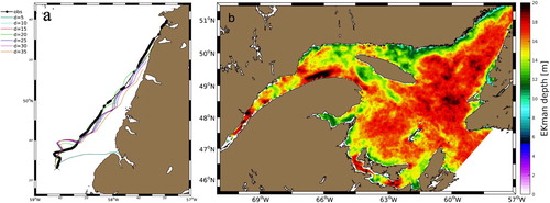
Model C has one free parameter which is the Ekman depth d. Using Equation (19(19) $d={\delta }_1(\nu =0)=\frac{z_2-z_1}{\ln \left[⟨\frac{\left|{\mathit{u}}_{\mathrm{a}\mathrm{g}}\left(z_2\right)\right|}{\left|{\mathit{u}}_{\mathrm{a}\mathrm{g}}\left(z_1\right)\right|}⟩\right]}$(19) ) with the ageostrophic currents obtained from GSL5km-RDPS, we computed the Ekman depth for all data points and we obtained $d\simeq 23\pm 15$ m ($\mathrm{m}\mathrm{e}\mathrm{a}\mathrm{n}\pm \mathrm{s}\mathrm{t}\mathrm{a}\mathrm{n}\mathrm{d}\mathrm{a}\mathrm{r}\mathrm{d}\mathrm{d}\mathrm{e}\mathrm{v}\mathrm{i}\mathrm{a}\mathrm{t}\mathrm{i}\mathrm{o}\mathrm{n}$). Before selecting one value in particular, we further evaluated the sensitivity of model C by comparing trajectories computed with different Ekman depth values between 5 and 35 m, with one trajectory taken from the drift data. Figure 4(a) shows that trajectories converge for Ekman depth values between 10 and 30 m, showing that the model is quite insensitive to this parameter in a fairly wide range. We thus choose d = 20 m for all our simulations. For small (5 m) and large (35 m) values, not only the simulated trajectories are shorter, but they tend to diverge from those obtained with intermediate values that are closer to observations. Figure 4(b) shows an example of daily-averaged Ekman depth values in the EGSL and how it is spatially distributed. Model D has also one free parameter which is time average of the speed of surface drifters relative to wind speeds, $q$. It has been determined from our observations as mentioned in the previous section.

Figure 4. (a) Buoy trajectories simulated using model C for different values of Ekman depth d, compared to the observed trajectory in the portion of the Gulf of St. Lawrence west of Newfoundland (black dots and line). (b) Daily-averaged Ekman depth calculated with Equation (19(19) $d={\delta }_1(\nu =0)=\frac{z_2-z_1}{\ln \left[⟨\frac{\left|{\mathit{u}}_{\mathrm{a}\mathrm{g}}\left(z_2\right)\right|}{\left|{\mathit{u}}_{\mathrm{a}\mathrm{g}}\left(z_1\right)\right|}⟩\right]}$(19) ) for 2 June 2014.

The wind correction coefficient ${\alpha }_i$ must be computed for each model $i=\mathrm{A}$, B, C, D as their respective Eulerian current velocities take up a different portion of the wind effect. We proceed by calculating the velocity vector difference between the observed drift and the Eulerian current velocity of model i, given as ${\mathit{\epsilon }}_{\mathit{i}}={\mathit{u}}_{\mathrm{o}\mathrm{b}\mathrm{s}}-{\mathit{u}}_{E0}^i$ for models B-D and ${\mathit{\epsilon }}_{\mathit{A}}={\mathit{u}}_{\mathrm{o}\mathrm{b}\mathrm{s}}-{\mathit{u}}_{E1}$ for model A. Then, ${\alpha }_i$ is obtained as the slope of the complex linear regression between ${\epsilon }_i$ and the wind velocity vector ${\mathit{U}}_{10}$. Values for each model are reported in Table 1. The 4th-order Runge-Kutta method is used to integrate the drift trajectories with a 1-h time step, a value below which solutions are practically similar and that preserve computational efficiency. Wind and current inputs are available at an hourly frequency and are linearly interpolated in time and space to the predicted drifter location. To compare the observed and predicted drifter velocities, we linearly interpolate wind and current velocities at the observed drifter locations. The tidal and geostrophic components are extracted from the total current and are interpolated separately.

2.5. Metrics

We assess the performance of the drift models against observations using different metrics: the complex correlation coefficient and the instantaneous angle difference between the observed and simulated drift velocities, the separation distance between the observed and simulated trajectories, and an aggregated skill score. Following Kundu (1976), let ${\mathit{u}}_{\mathrm{o}\mathrm{b}\mathrm{s}}\left(t\right)=u_{\mathrm{o}\mathrm{b}\mathrm{s}}\left(t\right)+i{v}_{\mathrm{o}\mathrm{b}\mathrm{s}}\left(t\right)$ be the complex representation of the 2D drifter velocity vector at the time t, and ${\mathit{u}}_d\left(t\right)=u_d\left(t\right)+i{v}_d\left(t\right)$ the complex representation of the velocity vector simulated by a drift model.

The complex correlation coefficient between these two series of vectors is(25) $\mathit{r}=\frac{⟨{\mathit{u}}_{\mathrm{o}\mathrm{b}\mathrm{s}}^{\ast }\left(t\right)\cdot {\mathit{u}}_{\mathrm{d}}\left(t\right)⟩}{⟨{\mathit{u}}_{\mathrm{o}\mathrm{b}\mathrm{s}}^{\ast }\left(t\right)\cdot {\mathit{u}}_{\mathrm{o}\mathrm{b}\mathrm{s}}\left(t\right){⟩}^{1/2}⟨{\mathit{u}}_{\mathrm{d}}^{\ast }\left(t\right)\cdot {\mathit{u}}_{\mathrm{d}}\left(t\right){⟩}^{1/2}}$(25) where the asterisk indicates the complex conjugate. We can write this complex correlation as $\mathit{r}=\left|\mathit{r}\right|\exp \left(\mathrm{i}\theta \right)$ where θ is the phase of the complex correlation.

The angle difference between velocity vectors ${\mathit{u}}_{\mathrm{o}\mathrm{b}\mathrm{s}}\left(t\right)$ and ${\mathit{u}}_{\mathrm{d}}\left(t\right)$ is noted $\phi \left(t\right)$ and follows the trigonometric convention (counterclockwise) with respect to the drifter velocity, such that a positive (negative) value means that the simulated velocity is to the left (right) of the observed velocity. The separation distance between observed and simulated drift trajectories, respectively $(x_{\mathrm{o}\mathrm{b}\mathrm{s}},y_{\mathrm{o}\mathrm{b}\mathrm{s}})$ and $(x_d,y_d)$, is noted $ds\left(t\right)$ and is used by many authors (e.g. Price et al. 2006; Barron et al. 2007; Caballero et al. 2008; Huntley et al. 2011; Cucco et al. 2012).

The skill score of a drift model and is defined as(26) $ssc=\left\{\begin{array}{l}1-sc\mathrm{i}\mathrm{f}sc⩽1\\ 0\mathrm{i}\mathrm{f}sc>1.\end{array}\right.$(26) where sc is the normalised cumulative Lagrangian separation distance given by(27) $sc=\frac{\sum _{n=0}^{N}d{s}_n}{\sum _{n=0}^N\sum _{m=0}^{n}d{l}_m}.$(27) The indices $n,m=0,\dots ,N$ denominate observation points along the trajectory, $d{s}_n$ are the distances between the observed and simulated positions and $d{l}_m$ are the distances between two consecutive positions on the observed trajectory. Low values of $sc$ means that a model simulates observations well. This has been proposed by Liu and Weisberg (2011) and used by others (Ivichev et al. 2012; Röhrs et al. 2012; De Dominicis et al. 2013), to evaluates entire trajectories cumulatively.

A skill of 1 means a perfect agreement between simulations and observations all along the trajectory (Röhrs et al. 2012). The bootstrap method is used to evaluate the uncertainty associated with these statistical parameters, using a thousand samples with replacement for each dataset. Results are given in Table 1. A large number of data points is needed in order to sample a variety of metoceanic conditions.

3. Results

In order to gain confidence with the chosen transfer functions, we first compare the ageostrophic current component of the GSL5km-RDPS at $z=z_1$, as obtained with Equation (11(11) ${\mathit{u}}_{\mathrm{a}\mathrm{g}}(z_1,t)=\mathit{u}(z_1,t)-{\mathit{u}}_{\mathrm{g}}(z_0,t)-{\mathit{u}}_{\mathrm{t}\mathrm{i}\mathrm{d}\mathrm{e}}(z_1,t).$(11) ), with the wind-induced ageostrophic current obtained as the inverse Fourier transform of Equation (10(10) $\mathit{U}(\nu ,z)=\mathit{H}(\nu ,z)\mathit{T}\left(\nu \right)$(10) ) evaluated at $z=z_1$, applied with both transfer functions. This is shown in Figure 5(b) for one particular buoy. Results indicate that the transfer functions allow for a reasonably good estimation of the surface ageostrophic dynamics of the model, and that they can advantageously be used to extrapolate the ageostrophic residual current of the GSL5km-RDPS model to the surface.

Figure 5. Time series of relevant quantities extracted along the observed and simulated drifting trajectory of Figure 4. (a) Vertical shear magnitude S between the top two cells of the GSL5km-RDPS along the observed trajectory. (b) The ageostrophic current magnitude $\left|{\mathit{u}}_{\mathrm{a}\mathrm{g}}^{\mathrm{M}\mathrm{o}\mathrm{d}\mathrm{e}\mathrm{l}}\right|$ estimated from the total current of the GSL5km-RDPS using Equation (11(11) ${\mathit{u}}_{\mathrm{a}\mathrm{g}}(z_1,t)=\mathit{u}(z_1,t)-{\mathit{u}}_{\mathrm{g}}(z_0,t)-{\mathit{u}}_{\mathrm{t}\mathrm{i}\mathrm{d}\mathrm{e}}(z_1,t).$(11) ) (red), and the wind-induced surface currents $\left|{\mathit{u}}_{\mathrm{a}\mathrm{g}}^{\mathrm{C}}\right|$ and $\left|{\mathit{u}}_{\mathrm{a}\mathrm{g}}^{\mathrm{D}}\right|$ estimated with transfer functions ${\mathit{H}}_{\mathrm{C}}$ and ${\mathit{H}}_{\mathrm{D}}$ and wind stress, respectively, using Equation (10(10) $\mathit{U}(\nu ,z)=\mathit{H}(\nu ,z)\mathit{T}\left(\nu \right)$(10) ). (c) Observed drift speed (black) and predicted by models A-D.

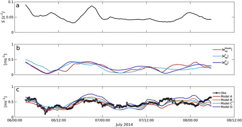
The main difference between the three extrapolation methods considered is the resulting shear between 0 and 2.5 m (Figure 3(a)), with model B yielding the weakest shear and model D the strongest. Therefore, the extrapolated surface currents are stronger than the model currents at 2.5 m, the surface currents obtained by model D being the strongest. After adding the wind correction, differences between the predicted drift speeds are sometimes reduced, but also sometimes increased (Figure 5(c)).

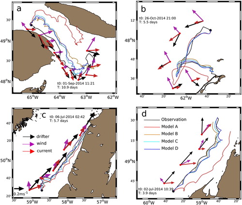
Despite the remaining discrepancies between predicted and observed drift velocities, predicted trajectories are closer to the observed trajectory for this particular drifter for models B-D (Figure 6(c,d)). Two other examples of drifting trajectories are shown in Figure 6 at different locations in the EGSL and at different times, in various conditions. While the trajectories predicted by model A using the model currents at 2.5 m sometimes depart far from the observed trajectories (e.g. in Figure 6(a)), the trajectories predicted by models B-D using currents extrapolated to the surface remain much closer. From these few examples, however, it is difficult to assess which of these models perform best in all situations. Therefore, a systematic assessment of the skills of the different drift models is carried out below using the metrics defined in Section 2.5, based on 40 trajectories with a total of 58,612 data points (Figure 2).

Figure 6. Examples of observed trajectories for four drifters (black line) (a, b, c, d) and trajectories simulated by model A (red), model B (brown), model C (light blue) and model D (dark blue). Drifter (black), wind (magenta) and current (red) daily-averaged velocity vectors are indicated along the trajectories.

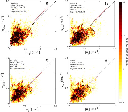
The amplitudes of the complex correlation coefficients between the predicted and observed drift velocity vectors increase from $\left|\mathit{r}\right|=0.61$ for model A to $\left|\mathit{r}\right|=0.77$ for model D (Figure 7). Therefore, surface drift is better predicted when explicitly extrapolating the top cell model currents to the surface, rather than solely relying on the parameterised wind correction term to account for the unresolved surface shear. While a simple linear extrapolation based on the shear between the two top model cells (model B) brings a modest improvement ($\left|\mathit{r}\right|=0.69$), the extrapolation methods based on Ekman dynamics (models C and D) bring further improvements ($\left|\mathit{r}\right|=0.73$ and $\left|\mathit{r}\right|=0.77$, respectively). However, the complex regression slope magnitudes indicate that predicted speeds are slightly overestimated on average by drift models which are based on extrapolated currents, while they were slightly underestimated by the control model.

Figure 7. Scatter plots between simulated and observed drift speeds for models A to D.

In addition to drift speed, drift direction must be well predicted to obtain accurate forecasts. Figure 8 shows the histograms of the difference between the instantaneous directions predicted by the drift models and the observed φ. For model A, the distribution peaks between $-{15}^{\circ }$ and $-5^{\circ }$, with a mean value of $-{3.2}^{\circ }$, indicating that predicted directions are biased on average to the right of observed directions. The spreading of the distribution is quite large with a standard deviation of 57.5${}^{\circ }$. Using extrapolation methods (models B-D), drift directions are improved: the distributions peak between $-{10}^{\circ }$ and ${10}^{\circ }$, and both the mean values and standard deviations are reduced. The best results are obtained for model D, with a mean value of ${1.3}^{\circ }$ and a standard deviation of ${42.5}^{\circ }$.

Drift speed and direction are instantaneous properties of drifters. Accurate forecasts require that they are consistently well predicted over the entire period of the forecast. To assess this, we computed separation distances ds between predicted and observed trajectories. The results are aggregated in Figure 9 and Table 1 for different forecast periods ranging from 3h to 72h. As one might expect, the separation distance increases as model errors integrate with time. For all forecast periods, model A performs the poorest while model D performs the best. The difference between models' performance is greater for shorter forecast periods: for 3-h forecasts, the mean separation distance ranges from 1.5 km for model A to 0.8 km for model D, a 41% improvement, while for 72-h forecasts, the mean separation distance ranges from 21 km for model A to 16 km for model D, a 24% improvement. The improvement of the mean separation distance for models B-D relative to model A, defined as ${\mathrm{\Delta }}_{\mathrm{A}i}=⟨(d{s}_{\mathrm{A}}-d{s}_i)/d{s}_{\mathrm{A}}⟩\times 100\text{\%}$, $i=$ B-D, is shown in Table 1. The simple linear extrapolation method (model B) already brings an improvement of about 25% with no significant trend as the forecast period increases. The extrapolation methods based on Ekman dynamics (models C and D) bring further improvement of about 31% and 35% respectively, which decreases with increasing forecast period. The improvement difference between models C and D is only a few percents. As seen from Figure 9, the median separation distance does not significantly improve beyond 12 hours, but the spread of the distribution (especially the 75th percentile) and extreme values are different even after 72 hours, which indicates that the probability to make large errors is reduced.

Figure 8. Histograms of the instantaneous angle difference between the observed and simulated drift velocity vectors $\phi$ comparing models (a) A (red) and B (brown), (b) A and C (light blue) and (c) A and D (purple). The mean ${\mu }_i={⟨\phi ⟩}_i$ and the standard deviation ${\sigma }_i$ are given for each model $i=\mathrm{A}-\mathrm{D}$.

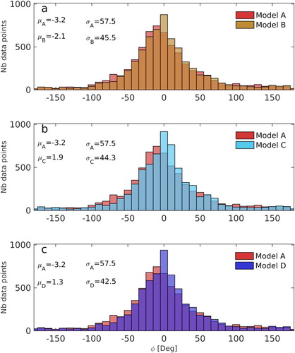
Figure 9. Box and whisker plots of the separation distance between observed and simulated trajectories for models A-D for different drift forecast periods. The horizontal line represents the median (50th percentile), box limits represent the 25th and 75th percentiles, and the whiskers represent extreme values.

The skill score defined in Section 2.5 (Equation (26(26) $ssc=\left\{\begin{array}{l}1-sc\mathrm{i}\mathrm{f}sc⩽1\\ 0\mathrm{i}\mathrm{f}sc>1.\end{array}\right.$(26) )) normalises the separation distance by the length of the drift trajectories, allowing to compare model skills at different forecast periods. Skill scores are reported in Table 1. The poorest skills are obtained by model A, while the best skills are obtained by model D for all forecast periods, reaching 0.89 for 3-h forecasts. Skill scores tend to decrease with increasing forecast period, albeit not monotonically, decreasing to 0.79 for 72-h forecasts for model D.

4. Discussion and conclusion

The formulation that is traditionally used in operational oceanography for predicting surface drift consists in adding a fraction of the 10-m wind velocity to the ocean currents provided in the centre of the top grid cell of an ocean circulation model, mathematically expressed as in Equation (3(3) ${\mathit{u}}_{\mathrm{d}}={\mathit{u}}_{E1}+\alpha {\mathit{U}}_{10}$(3) ). This wind correction term is supposed to account for many processes including windage, unresolved ocean current vertical shear, and wave-induced drift. In this study, we hypothesise that the vertical shear of the horizontal current in the upper ocean makes up for a significant part of the many wind-related contributions to the surface drift, and is not well taken into account by the wind correction term.

To test this hypothesis, we used two methods to extrapolate ocean currents taken from an ocean circulation model at known depths below the surface, to the surface. The extrapolated surface current replaces the ocean current in Equation (3(3) ${\mathit{u}}_{\mathrm{d}}={\mathit{u}}_{E1}+\alpha {\mathit{U}}_{10}$(3) ) and a new wind correction complex coefficient α is calculated. The first method (model B) uses a simple linear vector extrapolation and assumes that the near-surface shear is the same as the shear between the first two model grid cells. The second method assumes that the vertical shear is given by the wind-driven component of the current in Ekman balance with the time-varying wind and a prescribed diffusivity profile. Here we chose to test this method with constant (model C) and linear (model D) diffusivity profiles. We treat operational ocean and atmospheric models as black boxes providing ocean current and wind inputs to our drift models, with unknown biases and random errors. Hence our goal is to determine if drift forecast performances can be improved without increasing model resolution, model complexity and/or computational cost of these models.

Results show that using extrapolated surface currents instead of currents of the top grid cell of the ocean model significantly increases complex correlation with observed drift and decreases the value of α (both amplitude and phase). This means that our buoys are more driven by the surface current than the wind, and the near-surface wind-driven vertical shear can't simply be accounted for by the wind correction term ($\alpha {\mathit{U}}_{10}$). However, even though the value of $\alpha$ is reduced by a factor of 2 between model A and D, it is not zero, which means that our buoys are subject to windage and/or that other wind-driven processes are involved, such as wave-induced drift. Note that we determine the value of α using a complex linear regression, allowing rotation in the wind correction term of the drift models. The fact that it is mostly real indicates that the missing wind-driven forcing of the surface drift is in the direction of the wind. This suggests that processes like windage or the Stokes drift that are both aligned with the local wind might account for the residual wind correction term. The phase of α is small for all models but smallest for model D (see Table 1.).

Among the extrapolation methods we propose and study in this paper, the Ekman-based transfer function methods better represent the vertical shear than does a simple linear extrapolation. Indeed, models C and D outperform model B with respect to all performance metrics, supporting the idea that the wind-induced shear is consistent with the linearised horizontal momentum balance in the absence of horizontal pressure gradients (Elipot and Gille 2009). Also, model B requires knowledge of ocean currents at two depth levels. Model C requires knowledge about the Ekman depth, which is derived from currents at two depth levels. Model D, on the other hand, only needs one level, like model A. Models C and D outperform the two others, and among those two model D stands out for all metrics. Model D uses a linear diffusivity profile and has one tuning parameter ($q$, see Equation (21(21) $z_{\ast }=\frac{\kappa u_{\ast a}}{4f}\sqrt{\frac{{\rho }_a}{\rho }}\exp \left[-q\kappa \sqrt{\frac{\rho }{{\rho }_a}}\frac{\left|{\mathit{U}}_{10}\right|}{u_{\ast a}}\right]$(21) )). Model C uses a constant diffusivity profile and has also one tuning parameter ($d$, see Section 2.3). The test done by comparing the ocean model's ageostrophic current and the wind-induced current suggests that the parameterisation of $z_{\ast }$ is consistent with that of the model. Therefore, surface drift is better predicted when explicitly extrapolating the upper-cell model currents to the surface (models B-D), rather than solely relying on the parameterised wind correction term to account for the unresolved surface shear (model A). The chaotic nature of turbulent flows may explain why the improvement in terms of separation distances as a function of trajectory duration saturates with time (Figure 9). The median separation distance improves quite significantly for lead times shorter than 12 h compared to model A. For longer lead times, separation distance distributions for model B-D have a smaller upper tail, meaning that the probability of having predicted trajectories very far from the observed ones is reduced, which is desired in many particle tracking applications such as search and rescue.

Not only the drift models we propose here reduce biases compared to the standard model, but they remain computationally inexpensive. The computational cost associated with model D is 1.5 times the one associated with model A. Because both models C and D use variables that are already available and routinely produced by operational services, their implementation is straightforward and does not involve any modification to numerical modelling systems. Here we used the Canadian coupled atmosphere-ice-ocean forecasting system for the Gulf of St. Lawrence, with a vertical resolution of 5 m near the surface, which was the operational system at the time of the study. The upcoming Canadian operational system will be based on the Global Ice-Ocean Prediction System (GIOPS) and the associated nested regional configurations, that has a higher vertical resolution of 1 m near the surface (Smith et al. 2018). This may reduce the correction needed, as suggested by the results of Callies et al. (2017). Other model improvements such as coupling with atmospheric and wave models may also impact results. We thus suggest that the proposed improvements be viewed as a stop-gap measure until the operational model is updated, and a yardstick against which that new models can be assessed. Even with a higher vertical resolution, it is possible that extrapolating the vertical shear may still improve the surface drift forecasts (cf. Figure 3). Overall, because models C and D significantly improve all skill scores tested and that they are computationally affordable, we recommend extrapolating simulated near-surface Eulerian currents using the Ekman transfer function, and adjusting accordingly the wind correction term, as a way to improve drift forecasting skills and to improve response efficiency in all relevant applications.

Acknowledgements

Authors wish to thank Paul Nicot, Bruno Cayouette, the R/V Coriolis II crew during the Old Harry expedition in 2015, Comité ZIP Gaspésie and many volunteers all around the Gulf of St. Lawrence for their help in deploying and recovering drifting buoys. We also wish to thank the anonymous reviewers who helped improve the quality of the manuscript as well as the model performances with very useful advice.

Disclosure statement

No potential conflict of interest was reported by the authors.

Additional information

Funding

This work is funded by the Marine Environmental Observation, Prediction and Response (MEOPAR) Network of Centres of Excellence, Improving Marine Drift and Dispersion Forecasts (1-02-02-003.1), and by the Natural Sciences and Engineering Research Council of Canada (NSERC) Ship Time Grant Environmental conditions and dispersion processes within the Old Harry Influence Area (470204-2015). The project is a contribution to the research program of Québec-Océan.

References

- Al–Rabeh AH. 1994. Estimating surface oil spill transport due to wind in the Arabian Gulf. Ocean Eng. 21:461–465. doi: 10.1016/0029-8018(94)90019-1
- Al–Rabeh AH, Lardner RW, Gunay N. 2000. Gulfspill version 2.0: a software package for oil spills in the Arabian Gulf. Environ Model Softw. 15:425–442. doi: 10.1016/S1364-8152(00)00013-X
- Barron CN, Smedstad LF, Dastugue JM, Smedstad OM. 2007. Evaluation of ocean models using observed and simulated drifter trajectories: impact of sea surface height on synthetic profiles for data assimilation. J Geophys Res. 112(7):1–11.
- Blanke B, Raynaud S. 1997. Kinematics of the pacific equatorial undercurrent: an Eulerian and Lagrangian approach from GCM results. J Phys Oceanogr. 27:1038–1053. doi: 10.1175/1520-0485(1997)027<1038:KOTPEU>2.0.CO;2
- Bourgault D, Cyr F, Dumont D, Carter A. 2014. Numerical simulations of the spread of floating passive tracer released at the Old Harry prospect. Env Res Lett. 9(5):54001. doi: 10.1088/1748-9326/9/5/054001
- Bourgault D, Koutitonsky VG. 1999. Real-time monitoring of the freshwater discharge at the head of the st. Lawrence estuary. Atmos Ocean. 37(2):203–220. doi: 10.1080/07055900.1999.9649626
- Brandt G, Wehrmann A, Wirtz KW. 2008. Rapid invasion of Crassostrea gigas into the German Wadden Sea dominated by larval supply. J Sea Res. 59:279–296. doi: 10.1016/j.seares.2008.03.004
- Breivik Ø, Allen AA. 2008. An operational search and rescue model for the Norwegian Sea and the North Sea. J Mar Sys. 69(1–2):99–113. doi: 10.1016/j.jmarsys.2007.02.010
- Breivik Ø, Allen AA, Maisondieu C, Olagnon M. 2013. Advances in search and rescue at sea topical collection on advances in search and rescue at sea. Ocean Dyn. 63(1):83–88. doi: 10.1007/s10236-012-0581-1
- Breivik Ø, Allen AA, Maisondieu C, Roth JC. 2011. Wind-induced drift of objects at sea: the leeway field method 1. Appl Ocean Res. 33(1):100–109. doi: 10.1016/j.apor.2011.01.005
- Broche P, Demaistre J, Forget P. 1983. Mesure par radar décamétrique cohérent des courants superficiels engendrés par le vent. Oceanologica Acta. 6(1):43–53.
- Broström G, Carrasco A, Hole LR, Dick S, Janssen F, Mattsson J, Berger S. 2011. Usefulness of high resolution coastal models for operational oil spill forecast: the ‘Full City’ accident. Ocean Sci. 7:805–820. doi: 10.5194/os-7-805-2011
- Caballero A, Espino M, Sagarminaga Y, Ferrer L, Uriarte A, González M. 2008. Simulating the migration of drifters deployed in the Bay of Biscay, during the Prestige crisis. Mar Poll Bull. 56:475–482. doi: 10.1016/j.marpolbul.2007.11.005
- Callies U, Groll N, Horstmann J, Kapitza H, Klein H, Maßmann S, Schwichtenberg F. 2017. Surface drifters in the German Bight: model validation considering windage and Stokes drift. Ocean Sci. 13(5):799–827. doi: 10.5194/os-13-799-2017
- Chereskin T. 1995. Direct evidence for an Ekman balance in the California Current. J Geophys Res. 100:261–269.
- Cucco A, Sinerchia M, Ribotti A, Olita A, Fazioli L, Perilli A, Sorgente B, Borghini M, Schroeder K, Sorgente R. 2012. A high-resolution real-time forecasting system for predicting the fate of oil spills in the Strait of Bonifacio (western Mediterranean Sea). Mar Poll Bull. 64:1186–1200. doi: 10.1016/j.marpolbul.2012.03.019
- Daewel U, Schrum C, Gupta AK. 2015. The predictive potential of early life stage models (IBMs): an example for Atlantic cod Gadus morhua in the North Sea. Mar Ecol Prog Series. 534:199–219. doi: 10.3354/meps11367
- Davidson F, Allen A, Brassington G, Breivik Ø, Daniel Ø, Kamachi M, Sato S, King B, Lefevre F, Sutton M, Kaneko H. 2009. Applications of GODAE ocean current forecasts to search and rescue and ship routing. Environ Sci Technol. 3(22):176–181.
- De Dominicis M, Falchetti S, Trotta F, Pinardi N, Giacomelli L, Napolitano E, Fazioli L, Sorgente R, Haley PJ Jr, Lermusiaux PFJ, et al. 2014. A relocatable ocean model in support of environmental emergencies. Ocean Dyn. 64(9):667–688. doi: 10.1007/s10236-014-0705-x
- De Dominicis M, Leuzzi G, Monti P, Pinardi N, Poulain PM. 2012. Eddy diffusivity derived from drifter data for dispersion model applications. Ocean Dyn. 62(9):1381–1398. doi: 10.1007/s10236-012-0564-2
- De Dominicis M, Pinardi N, Zodiatis G, Archetti R. 2013. MEDSLIK-II, a Lagrangian marine surface oil spill model for short-term forecasting – Part 2: Numerical simulations and validations. Geosci Model Dev. 6:1871–1888. doi: 10.5194/gmd-6-1871-2013
- Döös K. 1995. Interocean exchange of water masses. J Geophys Res. 100(C7):13499–13514. doi: 10.1029/95JC00337
- Döös K, Meier HM, Dosche R. 2004. Royal Swedish Academy of Sciences. 33(3–4).
- Eide MS, Endresen Ø, Breivik Ø, Brude OW, Ellingsen IH, Røang K, Hauge J, Brett PO. 2007. Applications of GODAE ocean current forecasts to search and rescue and ship routing. Mar Poll Bull. 54(10):1619–1633. doi: 10.1016/j.marpolbul.2007.06.013
- Ekman VW. 1905. On the influence of the earth's rotation on ocean currents. Ark Mat Astr Fys. 2:1–36.
- Elipot S, Gille ST. 2009. Ekman layers in the Southern Ocean: spectral models and observations, vertical viscosity and boundary layer depth. Ocean Sci. 5(2):115–139. doi: 10.5194/os-5-115-2009
- Fernandez DM, Vesecky JF, Teague CC. 1996. Measurements of upper ocean surface current shear with high-frequency radar. J Geophys Res. 101(C12):28615–28625. doi: 10.1029/96JC03108
- Gästgifvars M, Lauri H, Sarkanen A, Myrberg K, Andrejev O, Ambjörn C. 2006. Modelling surface drifting of buoys during a rapidly-moving weather front in the Gulf of Finland, Baltic Sea. Estuarine Coast Shelf Sci. 70:567–576. doi: 10.1016/j.ecss.2006.06.010
- Gonella J. 1972. A rotary-component method for analysing meteorological and oceanographic vector time series. Deep-Sea Res. 19(12):833–846.
- Hackett B, Breivik Ø, Wettre C. 2006. Forecasting the drift of objects and substances in the oceans. In: Chassignet EP, Verron J, editors. Ocean weather forecasting: an integrated view of oceanography. Dordrecht: Springer; p. 507–523.
- Havens H, Luther ME, Meyers SD, Heil CA. 2010. Lagrangian particle tracking of a toxic dinoflagellate bloom within the Tampa Bay estuary. Mar Poll Bull. 60:2233–2241. doi: 10.1016/j.marpolbul.2010.08.013
- Henry LA, Mayorga-Adame CG, Fox AD, Polton JA, Ferris JS, McLellan F, McCabe C, Kutti T, Roberts MJ. 2018. Ocean sprawl facilitates dispersal and connectivity of protected species. Sci Rep. 8(1):11346. doi: 10.1038/s41598-018-29575-4
- Huntley HS, Lipphardt BL, Kirwan AD. 2011. Lagrangian predictability assessed in the East China Sea. Ocean Model. 36(1–2):163–178. doi: 10.1016/j.ocemod.2010.11.001
- Ivichev I, Hole RL, Karlin L, Wettre C, Röhrs J. 2012. Comparison of operational oil spill trajectory forecasts with surface drifter trajectories in the barents sea. Geol Geosci. 1:105.
- Jones CE, Dagestad KF, Breivik Ø, Holt B, Röhrs J, Christensen KH, Espeseth M, Brekke C, Skrunes S. 2016. Measurement and modeling of oil slick transport. J Geophys Res. 121:7759–7775. doi: 10.1002/2016JC012113
- Kjellsson J, Döös K. 2012. Surface drifters and model trajectories in the Baltic Sea. Boreal Env Res. 17(6):447–459.
- Kundu PK. 1976. Ekman veering observed near the ocean bottom. J Phys Oceanogr. 6(2):238–242. doi: 10.1175/1520-0485(1976)006<0238:EVONTO>2.0.CO;2
- Leppäranta M. 2011. The drift of sea ice. 2nd ed. Berlin, Heidelberg: Springer. (Springer Praxis books).
- Lequeux BD, Ahumada-Sempoal MA, López-Pérez A, Reyes-Hernández C. 2018. Coral connectivity between equatorial eastern Pacific marine protected areas: a biophysical modeling approach. PLoS ONE. 13(8):e0202995. doi: 10.1371/journal.pone.0202995
- Lewis DM, Belcher SE. 2004. Time-dependent, coupled, Ekman boundary layer solutions incorporating Stokes drift. Dyn Atmos Oceans. 37:313–351. doi: 10.1016/j.dynatmoce.2003.11.001
- Liu Y, Weisberg RH. 2011. Evaluation of trajectory modeling in different dynamic regions using normalized cumulative Lagrangian separation. J Geophys Res. 116(9):1–13.
- Maßmann S, Janssen F, Tborger B, Komo H, Kleine E, Menzenhauer-Schumacher I, Dick S. 2014. Operational ocean forecasting for German coastal waters. Kuste. 81(81):273–290.
- Masó M, Garcés E, Pagès F, Camp J. 2003. Drifting plastic debris as a potential vector for dispersing Harmful Algal Bloom (HAB) species. Sci Mar. 67(1):107–111. doi: 10.3989/scimar.2003.67n1107
- Mayorga–Adame GC, Batchelder HP, Spitz YH. 2017. Modeling larval connectivity of coral reef organisms in the Kenya-Tanzania region. Front Mar Sci. 4:92. doi: 10.3389/fmars.2017.00092
- Mellor GL, Yamada T. 1974. A hierarchy of turbulence closure models for planetary boundary layers. J Atmos Sci. 31(7):1791–1806. doi: 10.1175/1520-0469(1974)031<1791:AHOTCM>2.0.CO;2
- Paris CB, Le Hénaff M, Aman ZM, Subramaniam A, Helgers J, Wang DP, Kourafalou VH, Srinivasan A. 2012. Evolution of the Macondo well blowout: simulating the effects of the circulation and synthetic dispersants on the subsea oil transport. Environ Sci Technol. 46(24):13293–13302. doi: 10.1021/es303197h
- Pawlowicz R, Beardsley B, Lentz S. 2002. Classical tidal harmonic analysis including error estimates in MATLAB using T_TIDE. Comput Geosci. 28:929–937. doi: 10.1016/S0098-3004(02)00013-4
- Price JM, Reed M, Howard MK, Johnson WR, Ji ZG, Marshall CF, Guinasso NL Jr, Raineye GB. 2006. Preliminary assessment of an oil-spill trajectory model using satellite-tracked, oil-spill-simulating drifters. Environ Model Softw. 21:258–270. doi: 10.1016/j.envsoft.2004.04.025
- Price JF, Sundermeyer MA. 1999. Stratified Ekman layers. J Geophys Res. 104(C9):20467. doi: 10.1029/1999JC900164
- Röhrs J, Christensen KH, Håkon K, Vikebø F, Sundby S, Saetra Ø, Broström G. 2014. Wave-induced transport and vertical mixing of pelagic eggs and larvae. Limnol Oceanogr. 59(4):1213–1227. doi: 10.4319/lo.2014.59.4.1213
- Röhrs J, Christensen KH, Hole LR, Broström G, Drivdal M, Sundby S. 2012. Observation-based evaluation of surface wave effects on currents and trajectory forecasts. Ocean Dyn. 62(10–12):1519–1533. doi: 10.1007/s10236-012-0576-y
- Rudnick DL, Weller RA. 1993. Observations of superinertial and near-inertial wind-driven flow. J Phys Oceanogr. 23:2351–2359. doi: 10.1175/1520-0485(1993)023<2351:OOSANI>2.0.CO;2
- Saucier FJ, Roy F, Gilbert D, Pellerin P, Ritchie H. 2003. Modeling the formation and circulation processes of water masses and sea ice in the Gulf of St. Lawrence, Canada. J Geophys Res. 108(C8):2501–2520.
- Smith GC, Bélanger JM, Roy F, Pellerin P, Ritchie H, Onu K, Roch M, Zadra A, Colan DS, Winter B, et al. 2018. Impact of coupling with an ice-ocean model on global medium-range nwp forecast skill. Mon Weather Rev. 146(4):1157–1180. doi: 10.1175/MWR-D-17-0157.1
- Smith GC, Roy F, Brasnett B. 2012. Evaluation of an operational ice-ocean analysis and forecasting system for the Gulf of St Lawrence. Q J R Meteorol Soc. 139(671):419–433. doi: 10.1002/qj.1982
- Soomere T, Viikmäe B, Delpeche N, Myrberg K. 2010. Towards identification of areas of reduced risk in the Gulf of Finland, the Baltic Sea. Proc Estonian Academy Sci. 59(2):156–165. doi: 10.3176/proc.2010.2.15
- Starr M, Lair S, Michaud S, Scarratt M, Quillam M, Lefaivre D, Robert M, Wotherspoon A, Michaud R, Ménard N, et al. 2017. Multispecies mass mortality of marine fauna linked to a toxic dinoflagellate bloom. PLoS ONE. 12(5):e0176299. doi: 10.1371/journal.pone.0176299
- Van Sebille E, England MH, Froyland G. 2012. Origin, dynamics and evolution of ocean garbage patches from observed surface drifters. Env Res Lett. 7(4):044040. doi: 10.1088/1748-9326/7/4/044040
- Van Sebille E, Wilcox C, Lebreton L, Maximenko N, Hardesty BD, Franeker JAV, Eriksen M, Siegel D, Galgani F, Law KL. 2015. A global inventory of small fl oating plastic debris. Env Res Lett. 10(12). doi: 10.1088/1748-9326/10/12/124006
- Weller RA. 1981. Observations of the velocity response to wind forcing in the upper ocean. J Geophys Res. 86:1969–1977. doi: 10.1029/JC086iC03p01969