Development of small vessel advisory and forecast services system for safe navigation and operations at sea by N.D. Aditya, K.G. Sandhya, R. Harikumar and T.M. Balakrishnan

First, the discussers wish to compliment the authors, Aditya et al. (2022) (hereafter referred to as A22), on their results involving the development of a small vessel advisory and forecast services system for safe navigation and operation at sea for the Indian Ocean regime. These comments and discussion focus on the steepness index parameter ($I_s$) used within the Small Vessel Advisory Services (SVAS) system (see Figure 3 in A22) and point out that regional wave statistics can be used to determine and review the properties of $I_s$ in relation to significant wave height, allowing a robust method for determining and quantifying warning thresholds.

A22 used the steepness index as one of the three indices in the boat safety index (see Equation (6) in A22). The steepness index is given as (1) $I_s\equiv I_{steepness}={\displaystyle \frac{s_s}{0.05}\times {\displaystyle \frac{H_s}{h_0}={\displaystyle \frac{1}{c}{s}_s{H}_{s}c=0.05h_0}}}$(1) where $H_s$ is the significant wave height, $h_0$ is a region-specific constant value, $s_s=H_s/((g/2\pi )T_z^2)$ is the wave steepness defined in terms of $H_s$ and the mean zero-crossing wave period $T_z$, $g$ is the acceleration due to gravity, and the wave steepness value 0.05 corresponds to that for a Pierson–Moskowitz wave amplitude model spectrum. For the Indian Sea A22 used $h_0=2.5$ m, while Niclasen et al. (2010) used $h_0=4$ m representing North Sea conditions.

The statistical features of $I_s$ will be exemplified based on wave statistics obtained from the joint probability density function (pdf) of $H_s$ and $I_s$, provided in Appendix A, which is based on wave data from the northern North Sea. Thus it is consistent to use $h_0=4$ m representing North Sea conditions (Niclasen et al. 2010), that is, using $c=0.2$ in Equation (1).

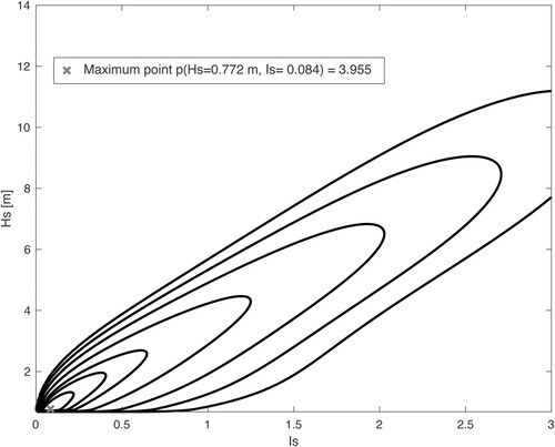
Figure 1 shows the isocontours of $p(H_s,I_s)$ with the contours p = 0.0001, 0.001, 0.01, 0.1, 0.5, 1, 2 from the outer to inner contours, respectively. Furthermore, the peak value p_max= 3.955 is located at $H_s$ = 0.722 m and $I_s$ = 0.084.

Figure 1. Isocontours of $p(H_s,I_s)$ with the contours p = 0.0001, 0.001, 0.01, 0.1, 0.5, 1, 2 from the outer to the inner contours, respectively.

Figures 2 and 3 show the conditional expected value of $I_s$ given $H_s$, $E[I_s|H_s]$ (Figure 2) and the corresponding conditional coefficient of variation $R[I_s|H_s]$ (Figure 3) versus $H_s$. From Figure 2, it appears that $E[I_s|H_s]$ increases as $H_s$ increases, reaching a value of about 3.7 for $H_s$ = 14 m. Figure 3 shows that $R[I_s|H_s]$ decreases as $H_s$ increases; from about 0.6 for $H_s$ about 1 m to about 0.01 for $H_s$ = 14 m.

Figure 2. $E[I_s|H_s]$ versus $H_s$.

Figure 3. $R[I_s|H_s]$ versus $H_s$.

Next, an example of results is given in terms of $E[I_s|H_s]$ and $R[I_s|H_s]$ where $H_s$ is obtained from Equations (A3) and (A15) as $E[H_s]=2.11$ m. Then, substituting this value of $H_s$ in Equations (A5)–(A8), (A10)–(A12) and (A14) gives ${\mu }_{I_s}=0.761$, ${\sigma }_{I_s}^2=0.0934$, $R=0.313$. Consequently, the mean value $\pm 1$ standard deviation interval of $E[I_s|E[H_s]=2.11\mathrm{m}]$ = 0.490 is 0.337–0.643.

Overall, in future applications of the SVAS system, it should be considered to implement the statistical properties of the waves, e.g. from global wave atlases such as Hogben et al. (1986) (see Appendix A).

Appendix A.

Joint pdf of $H_s$ and $I_s$

Here the joint probability density function (pdf) of $H_s$ and $I_s$ is obtained from the joint pdf of $H_s$ and $s_s$ given by Myrhaug (2018) (hereafter referred to as M18). This ($H_s$, $s_s$) distribution was deduced from the Mathisen and Bitner-Gregersen (1990) joint pdf of $H_s$ and $T_z$, obtained as a best fit to the observed scatter diagram based on data recorded by a wave buoy at the Utsira location (in the northern North Sea) on the Norwegian continental shelf during the years 1974–1986. The data represent deep water swell, wind waves, and combined swell and wind waves conditions.

It should be noted that the same results can be deduced directly from the joint pdf of $H_s$ and $T_z$ as explained in the last paragraph of this Appendix.

The joint pdf of $H_s$ and $s_s$ provided by M18 is given as (A1) $p(H_s,s_s)=p(s_s|H_s)p(H_s)$(A1) where $p(H_s)$ is the marginal pdf of $H_s$ with the following three-parameter Weibull pdf: (A2) $p(H_s)={\displaystyle \frac{{\theta }_h}{{\zeta }_h}{\left({\displaystyle \frac{H_s-{\epsilon }_h}{{\zeta }_h}}\right)}^{{\theta }_h-1}\exp \left[-{\left({\displaystyle \frac{H_s-{\epsilon }_h}{{\zeta }_h}}\right)}^{{\theta }_h}\right]H_s\ge {\epsilon }_h}$(A2) and the Weibull parameters (A3) ${\zeta }_h=1.50\mathrm{m},{\theta }_h=1.15,{\epsilon }_h=0.679\mathrm{m}$(A3) Furthermore, $p(s_s|H_s)$ is the conditional pdf of $s_s$ given $H_s$, given by the following lognormal pdf (A4) $p(s_s|H_s)={\displaystyle \frac{1}{\sqrt{2\pi }{\sigma }_{s_s}{s}_s}\exp \left[-{\displaystyle \frac{1}{2}{\left({\displaystyle \frac{ln{s}_s-{\mu }_{s_s}}{{\sigma }_{s_s}}}\right)}^2}\right]}$(A4) where ${\mu }_{s_s}$ and ${\sigma }_{s_s}^2$ are the mean value and the variance, respectively, of $ln{s}_s$, given as (A5) ${\mu }_{s_s}=ln\left({\displaystyle \frac{H_s}{g/2\pi }}\right)-2(a_1+a_2{H}_s^{a_3})$(A5) (A6) $a_1=0.933,a_2=0.578,a_3=0.395$(A6) (A7) ${\sigma }_{s_s}^2=4(b_1+b_2{e}^{b_3{H}_s}{)}^2$(A7) (A8) $b_1=0.0550,b_2=0.336,b_3=-0.585$(A8)

Here $H_s$ is in metres in Equations (A5) and (A7) (see M18 for more details).

The statistical features of $I_s$ are derived by using this joint pdf of $(H_s,s_s)$ by changing of variables from $(H_s,s_s)$ to $(H_s,I_s)$, and the joint pdf of $(H_s,I_s)$ becomes $p(H_s,I_s)=p(I_s|H_s)p(H_s)$. Thus only $p(I_s|H_s)$ is affected since $s_s=c{H}_s^{-1}{I}_s$, which by transformation of variables gives a lognormal pdf of $I_s$ given $H_s$ as (i.e. by using the Jacobian $|d{s}_s/d{I}_s|=c{H}_s^{-1}$) (A9) $p(I_s|H_s)={\displaystyle \frac{1}{\sqrt{2\pi }{\sigma }_{I_s}{I}_s}\exp \left[-{\displaystyle \frac{{(ln{I}_s-{\mu }_{I_s})}^2}{2{\sigma }_{I_s}^2}}\right]}$(A9) The conditional expected value ${\mu }_{I_s}$ and the conditional variance ${\sigma }_{I_s}^2$ of $ln{I}_s$ are (A10) ${\mu }_{I_s}=ln\left({\displaystyle \frac{H_s^2}{cg/2\pi }}\right)-2(a_1+a_2{H}_s^{a_3})$(A10) ${\sigma }_{I_s}^2={\sigma }_{s_s}^2=4(b_1+b_2{e}^{b_3{H}_s}{)}^2$(A11)

The conditional expected value and the conditional variance of $I_s$ are obtained from the known $p(I_s|H_s)$ in Equation (A9) as (Bury 1975) (A12) $E[I_s|H_s]=\exp ({\mu }_{I_s}+{\displaystyle \frac{1}{2}{\sigma }_{I_s}^2)}$(A12) (A13) $Var[I_s|H_s]=(e^{{\sigma }_{I_s}^2}-1)\exp (2{\mu }_{I_s}+{\sigma }_{I_s}^2)$(A13) Then it follows that the conditional coefficient of variation is (A14) $R[I_s|H_s]={\displaystyle \frac{{(Var[I_s|H_s])}^{1/2}}{E[I_s|H_s]}=(e^{{\sigma }_{I_s}^2}-1{)}^{1/2}}$(A14)

Moreover, $E[H_s]$ is given as (Bury 1975) (A15) $E[H_s]={\epsilon }_h+{\zeta }_h\mathrm{\Gamma }(1+{\displaystyle \frac{1}{{\theta }_h})}$(A15) where $\mathrm{\Gamma }$ is the gamma function.

As referred to, the joint pdf of $H_s$ and $I_s$ can alternatively be obtained by transforming the joint pdf of $H_s$ and $T_z$, e.g. from the Mathisen and Bitner-Gregersen (1990) joint pdf $p(H_s,T_z)=p(T_z|H_s)p(H_s)$ where $p(T_z|H_s)$ is lognormal-distributed (see Equation (B3) in M18). From Equation (1), $I_s=(2\pi /cg)(H_s^2/T_z^2)$ by substituting for $s_s$, and accordingly $T_z=(2\pi /cg{)}^{1/2}{H}_s^{}{I}_s^{-1/2}$. Thus transformation from $T_z$ to $I_s$ using the Jacobian $|d{T}_z/d{I}_s|=(2\pi /cg{)}^{1/2}{H}_s^{}{I}_s^{-3/2}/2$ gives $p(I_s|H_s)$ as in Equation (A9). Then, similar results can be obtained for other ocean areas since joint statistics of $H_s$ and $T_z$ are available, e.g. from global wave atlases such as Hogben et al. (1986).

References

- Aditya ND, Sandhya KG, Harikumar R, Balakrishnan Nair TM. 2022. Development of small vessel advisory and forecast services system for safe navigation and operations at sea. J Oper Oceanograph. 15(1):52–67. doi:10.1080/1755876X.2020.1846267.
- Bury KV. 1975. Statistical models in applied science. New York: John Wiley & Sons.
- Hogben N, Duncan NMC, Olliver GF. 1986. Global wave statistics. London: Unwin Brothers.
- Mathisen J, Bitner-Gregersen E. 1990. Joint distributions for significant wave height and wave zero-up-crossing period. Appl Ocean Res. 12(2):93–103.
- Myrhaug D. 2018. Some probabilistic properties of deep water wave steepness. Oceanologia. 60(2):187–192. doi:10.1016/j.oceano.2017.10.003.
- Niclasen BA, Simonsen K, Magnusson AK. 2010. Wave forecasts and small-vessel safety: a review of operational warning parameters. Mar Struct. 23(1):1–21. doi:10.1016/j.marstruc.2010.02.001.
Appendix A.
Joint pdf of  and