Sediment accretion in a lower-energetic location during two consecutive cold fronts

ABSTRACT

During the passage of two consecutive atmospheric cold fronts that migrated eastward along the northern Gulf of Mexico, currents, waves, and seafloor elevation were observed from instrumentation attached to a metal structure called ‘quadpod’ at the 7.5 m bathymetric contour off the coast of Panama City, Florida. During the passage of the first front, significant wave height (Hs) increased from 0.15 m to 1.2 m, and seafloor elevation relative to the quadpod increased by up to 5 cm at the quadpod location. During the passage of the second front, Hs peaked at 2 m, and seafloor elevation increased by up to 15 cm over 24 h. The increase in the seafloor elevation is consistent with the burial of surrogate munitions observed with sonar imagery and with sediment accretion from a Delft3D simulation. The model predicts cross-shore seafloor changes with erosion nearshore and accretion offshore, starting at approximately 250 m from the coast. The seafloor elevation increase is attributed to sediment accretion driven by wave forcing. The results of this study have important implications for morphological changes and object burial during a period of front-driven waves in the northern Gulf of Mexico, which is typically a lower energetic environment.

KEYWORDS:

• Morphological modelling
• nearshore
• sandy seafloor
• Delft3D
• sediment accretion
• front-driven waves

1. Introduction

Waves and currents drive sediment transport, leading to the seafloor evolution through sediment accretion and erosion (Roelvink and Reniers, 2012). Field observations have demonstrated that high-energy storm waves can produce offshore sediment transport (Komar, 1976) and erode the coastline while wave-induced undertow currents carry sediment in the offshore direction forming sand bars (Van Rijn, 2013). These morphological effects can be accentuated during consecutive storms when the interval between storms is shorter than the beach recovery period for a single storm (Morton, 1995; Callaghan et al., 2008). In the initial storm phase, rapid erosion near the beach and nearshore bar are expected, along with gradual surf zone sediment redistribution (Vousdoukas et al., 2012). The second storm produces more extensive seafloor changes taking advantage of the destabilising effect of the first storm on the seafloor that does not have enough time to recover (Lee et al., 1998).

Accurate prediction of erosion and sediment accretion can reduce the costs of environmental remediation efforts aimed at recovering underwater munitions although it is very challenging. The U.S. Army Corps of Engineers, Navy, and Marine Corps have identified more than 430 locations in the United States as potentially containing underwater munitions with polluting potential (SERDP-ESTCP, 2010). From 2001 to 2005, the U.S. Office of Naval Research (ONR) fostered research on mine burial prediction through an Accelerated Research Initiative (ARI) (Bennett, 2000). As part of efforts to improve the risk assessment to remediation actions, six degrees of freedom (6-DoF) model named IMPACT35 was developed to predict the three-dimensional trajectory of sea mines (Chu et al., 2004, 2005; Chu and Fan, 2005, 2006; Chu, 2009) and refurbished into an underwater munition scour burial (UnMUSB) model to predict seafloor munition’s mobility and burial (Chu et al., 2021, 2022; Chu and Fan 2022). The UnMUSB model requires environmental parameters such as waves, currents, and sediment accretion/erosion in order to accurately predict the location, mobility, and burial of munition. Delft3D, a freely available open-source numerical model software package (Deltares, 2019a), is capable of providing the parameters required by UnMUSB.

Previous works on sedimentation and erosion caused by consecutive storms have studied high-energy storm events in typically higher-energetic locations (Lee et al., 1998; Ferreira, 2005; Callaghan et al., 2008; Vousdoukas et al., 2012), but not on moderate-energy storm events in lower-energetic locations. In this study, Delft3D is used to predict the measured seafloor elevation obtained at a single mooring over the mid-shelf off the coast of Panama City, Florida (lower-energetic location) and to identify the mechanisms responsible for the observed sediment accretion and erosion during the passage of two consecutive atmospheric cold fronts using observed significant wave heights, mean currents, and sonar images.

2. Field experiment

2.1. Study area

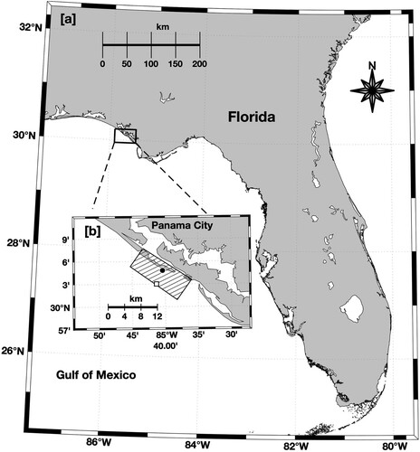
The study area, off the coast of Panama City, Florida, in the northern Gulf of Mexico (Figure 1), is considered a lower-energetic location (Calantoni et al., 2014), where the mean wave period is 8 s and the mean wave height is 0.9 m (Farrar et al., 1994). This area has a diurnal tide with a maximum tidal range of 0.4 m (Bunya et al., 2010) and seasonal winds primarily from the north in winter and fall and from the south in summer and spring with a weak mean wind speed of around 3 m/s (Chu et al., 2006). In the hurricane seasons, from June to November, high waves and surges associated with sporadic storms can cause significant morphologic changes on the coast of Panama City (Taiani et al., 2012). The sedimentation is primarily quartz sand with a grain density of approximately 2,650 kg/m³ (Plant et al., 2013). The sediment collected during TREX13 is within the fine sand category at the shallow quadpod location (solid dot in Figure 1b).

Figure 1. Northern Gulf of Mexico. (a) The location of the coast of Panama City is indicated by the black rectangle. (b) The study area is highlighted by the hatched rectangle. The black dot represents the location of the shallow quadpod at 30° 04.81’ N, 85° 40.41’ W, and the white square denotes the deep quadpod location at 30° 03.02’ N, 85° 41.34’ W.

2.2. Instrumentation

During the TREX13 in April and May 2013, two metal structures called shallow and deep quadpods were deployed cross-shore on 20 April with attached oceanographic instrumentation. The shallow quadpod is approximately 2.3 m tall at the water depth of 7.5 m (black dot in Figure 1b), and the deep quadpod is approximately 3.3 m tall at the water depth of 20 m (white dot in Figure 1b). Non-explosive surrogate munitions with different sizes and densities were placed on the seafloor in both quadpod locations (Calantoni et al., 2014). Locations of surrogates along with seafloor topography were recorded once every 12 min by a 2.25 MHz sector scanning sonar Imagenex 881 at 105 cm above the seafloor with 110 degrees of azimuth and 6 m range. Horizontal currents were measured for 20 min every half hour at 2 Hz from the top of each quadpod to the surface at 50 cm vertical resolution by upward-looking Nortek AWAC 1 MHz acoustic Doppler current profilers (ADCP) at 2.3 m above the seafloor. Mean currents were computed from the hourly depth-averaged flow. The mean water level, significant wave height (highest one-third of waves), mean wave direction, and peak wave period were estimated from AWAC pressure data. Additionally, the seafloor elevation was measured by the identified depth of maximum backscatter from a faced down 1.5 MHz Sontek pulse coherent acoustic Doppler profiler (PC-ADP) at 80 cm above the seafloor. The PC-ADP also continuously measured the seafloor up to 80 cm and the suspended sediment concentration with 5 cm bins of spatial resolution and 2 Hz of temporal resolution. All equipment was retrieved on 23 May 2013.

2.3. Time series of observed data

Considerable modifications in the seafloor were observed during TREX13 after the passage of two consecutive cold fronts in early May 2013. The evolution of current magnitude, significant wave height, and sediment accretion at the shallow quadpod are provided in Figure 2. The gray stripes in Figure 2a and b represent the two periods of sediment accretion corresponding to the first and second cold front passages. The oceanographic conditions before 4 May (i.e. before front passage) represented typical lower-energetic features with weak hourly averaged current speed ranging between 0.01 and 0.15 m/s (Figure 2a), and small significant wave height ranging between 0.2 and 0.5 m (Figure 2b). The significant wave height increased to 1.2 m during the first cold front passage and reached 2 m during the second front passage. The seafloor elevation (black line in Figure 2c) was measured from the PC-ADP maximum backscatter of the water column from the seafloor up to 0.6 m, and increased approximately 5 and 15 cm during the first and second cold front passages. Suspended sediment in the water column is also observed (greenish backscatter) starting from the first front passage. The backscatter of suspended sediment is even stronger (yellowish/reddish) during the second front passage, indicating that sediment transport is likely increasing.

Figure 2. Time series of (a) observed current magnitude (1h-average), (b) observed significant wave height, and (c) seafloor elevation (black curve) from the PC-ADP maximum backscatter of the water column from the seafloor up to 0.6 m (colour plot) from 3 to 5 May. The periods highlighted in gray represent the two periods of sediment accretion at the shallow quadpod location and correspond to the first and second cold front passages.

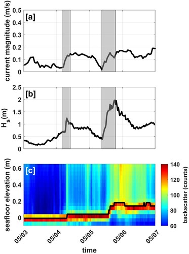
In both front passages, sediment accretion and significant wave height increased simultaneously. Such an apparent synchronisation between wave and sedimentation and the weak currents associated with the two cold front passages (Figure 2) suggest that waves primarily drive the observed morphological changes. Although similar conditions of waves and currents were observed at the deep quadpod, the seafloor elevation changes were not evident.

Klammler et al. (2021) used a poroelastic wave-sediment interaction model to infer that the 15 cm increase in seafloor elevation identified from the PC-ADP maximum backscatter (shown in Figure 2c) is a result of sediment liquefaction by loss of vertical effective stress. In addition, they estimated a 10 cm sinking of the quadpod into the sediment during the passage of the second cold front and recognised the uncertainty about the contributions of bedform migration and scour for the observed morphological data shown in Figure 2c. We use a well-known numerical model, Delft3D, to supplement their contributions to explain the observed increase in seafloor elevation.

3. Modelling system

The open-source modelling system Delft3D (Lesser et al., 2004) version 4.04.01 is implemented to predict currents, waves, sediment transport, and morphological evolution in the nearshore environment off the coast of Panama City. The flow module (Delft3D-Flow), either two-dimensional or three-dimensional, is forced by tides, winds, and density, predicts the currents and feeds the current data as input into the wave and morphology modules (Deltares, 2019a). In addition, the flow module is also able to predict suspended sediment transport, bedload transport, and bathymetric variation for both cohesive (e.g. silt and clay) and non-cohesive (e.g. gravel and sand) sediments through solving the advection–diffusion equation with the empirical formulation. However, this study is limited to the sandy seafloor. The cohesive sediments are not included. The wave module (Delft3D-Wave) uses a third-generation model ‘Simulating Waves Nearshore (SWAN)’ derived from an Eulerian wave action balance equation (Booij et al., 1999) to predict the wave generation, propagation, dissipation, and non-linear wave-wave interactions with inputs from the flow module such as water level, bathymetry, wind, and currents (Deltares, 2019b). The morphology module (Delft3D-MOR) is an integrated process-based model to predict the bathymetric change under impact of waves, currents, and sediment transport from the flow and wave modules. The bathymetric change feeds back to the flow and wave modules, and the loop restarts. Similar to earlier studies in this area (Pessanha, 2019; Chu et al., 2021), the model grids and tide-forcing boundary conditions are identified in the Delft Dashboard (DDB), which is based on MATLAB and integrated into Delft3D. Our study area is considered vertically well mixed. Hence, the two-dimensional barotropic model approach is adopted.

3.1. Grids, bathymetry, and wind input

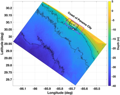
Two uniform grids with different resolutions for the flow module are nested (Figure 3) to create outer and inner grids. The outer grid (coarser resolution) is 137×75 with 50 m resolution in both alongshore and cross-shore directions. The inner grid (finer resolution) is 139 ×124 with a 20 m resolution. The sediment transport and morphological evolution are computed only in the inner grid of the flow module to compare with the TREX13 measurements. The domain for the wave module (Figure 3) is determined to avoid the boundary effect and allow the use of deep quadpod data to set up the wave boundary conditions. The wave grid is 273×111 with a 50 m resolution. The bathymetric data (Figure 3) is from the Northern Gulf Coast Digital Elevation Model from the National Oceanic and Atmospheric Administration/National Geophysical Data Centre (NOAA/NGDC) (NOAA/NGDC, 2010). The resolution of this data set varies between 1/3 and 1 arc-second (around 10 and 30 m). The wind input files are set up using the ERA5 Reanalysis data from the European Centre for Medium-Range Weather Forecasts (ECMWF), with a 0.25° (around 28 km) resolution (ECMWF, 2019).

Figure 3. Bathymetry, depth contours (10, 20, 25, and 35 m), wave (magenta), flow outer (black), and flow inner (white) computational grids enclosures are indicated on the map. The black dot represents the shallow quadpod location, and the white square denotes the deep quadpod location.

3.2. Initial and boundary conditions

Global Inverse Tide Model TPXO 8.0, included in the DDB, is used to create the boundary conditions for the flow module. For the alongshore boundary, the water level is imposed with the astronomic forcing. The water level gradient is set up to zero open boundaries (a so-called Neumann boundary condition). It allows for the flow to leave and enter the lateral boundaries with no spurious circulation (Roelvink and Walstra, 2004). The water level is set to zero initially. Additionally, the boundary conditions for sediment transport are set by specifying the inflow concentration as 0 kg/m³. The initial condition for the sediment concentration is set as 0 kg/m³, and the initial bed of sediment is set to 5 m. The wave boundary conditions are set based on the measurements from the deep quadpod location using the significant wave height, wave period, wave directions, and directional spreading. These parameters are applied uniformly on the three open boundaries.

3.3. Calibration and model parameters

The calibration is directed to adjust the parameters and allow a better agreement between the model output and measurements. The period between 21 and 27 April is selected for calibration due to observed significant variations in water level, waves, and currents. During the calibration, the model-generated water level, waves, and currents are compared to the observations, and model parameters are adjusted individually, with one being fine-tuned and others remaining unchanged.

Typically, the water level is calibrated by adjustments in the boundary conditions. However, since the minimal difference is reached in amplitude and phase between modelled and measured tides, no boundary condition adjustment is required to calibrate the water level. The waves are calibrated with different JONSWAP bottom friction coefficients and wave height to water depth ratio (γ) in the depth-induced breaking model (Battjes and Janssen, 1978) and with adjustments in the boundary conditions. The Chézy friction coefficient is calibrated with flow velocities. Based on the Courant–Friedrichs–Lewy number, the time step is set as 0.2 s for the coarse domain (50 m) and 0.1 s for the detailed domain (20 m). The model used a uniform Chézy bottom roughness of 65 m^1/2/s. Horizontal eddy viscosity and horizontal eddy diffusivity were set as 0.5 and 10 m²/s, respectively.

The computational mode for waves is set as stationary. Also, the coupling time between the flow and wave modules is set to 60 min. The JONSWAP model (Hasselmann, 1974) is used to calculate the bottom friction component of wave dissipation with constant bottom friction. Also, the depth-induced breaking (Battjes and Janssen, 1978) is set with α equal to 1 and γ equal to 0.73. The model has a directional resolution of 5° and 24 frequency bins from 0.05 Hz to 1 Hz.

The spin-up interval of 720 min is established to prevent any influence of a possible initial hydrodynamic instability on the bottom change calculation, which starts only after the spin-up interval. The sediment type is set as sand with a sediment-specific density of 2,650 kg/m³.

4. Results and discussion

4.1. Consecutive cold fronts

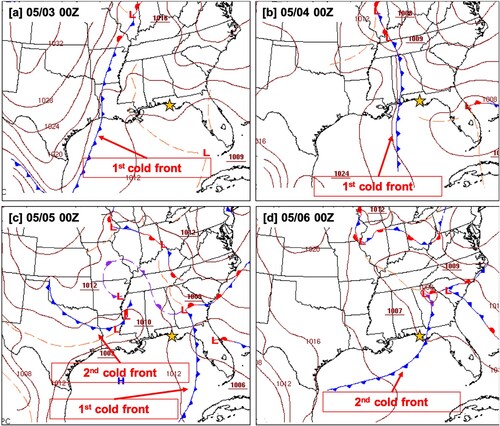
Between 4–6 May, two cold fronts passed through Panama City, driving northward swell associated with winds from the south following the historical pattern of frontal incursions into the Gulf of Mexico (DiMego et al., 1976; Guo et al., 2020). Figure 4 presents a sequence of surface weather maps from the Weather Prediction Centre website (NOAA/WPC, 2020) from 3 to 6 May. On 3 May, the first cold front extended from Arkansas to the southern U.S. and moved across Louisiana towards Florida (Figure 4a). The first cold front reached Panama City between 4–5 May (Figure 3b) and coincided with maximum significant wave heights of 1.2 m and a peak wave period of 10 s observed at the shallow quadpod location. On 5 May, the second front extended over northern Texas (Figure 4c), and crossed over Panama City between 5–6 May (Figure 4d), causing higher wave conditions. For the second cold front passage, observations at the shallow quadpod location exhibit significant wave heights of 2 m and a peak wave period of 7 s for the second cold front passage.

Figure 4. Surface analysis including passage of cold fronts through the northern Gulf of Mexico during 3–6 May 2013. The first cold front reached Panama City (highlighted by the yellow star) between 4–5 May and the second front between 5–6 May. Adapted from (NOAA/WPC, 2020).

4.2. Model performance

The model performance is quantified by skill score (Willmott, 1981), relative mean absolute error (RMAE) (Van Rijn et al., 2003), root-mean-squared error (RMSE), and bias. The skill score reveals the level of the accuracy of the model in estimating the observed variable. The skill score is 1 for the perfect agreement and 0 for the complete disagreement between the modelled and observed data. Table 1 shows a qualification of error ranges based on wave height and current magnitude (Van Rijn et al., 2003), and Table 2 condenses the statistical guidelines to determine the minimum performance of a model based on RMSE and bias (Williams and Esteves, 2017). The model capability to predict the quick increase of sediment is evaluated using observed PC-ADP maximum backscatter data, and quantified by the Brier Skill Score (BSS) (Van Rijn et al., 2003) (shown in Table 3). The model performance is evaluated using the data collected at the shallow quadpod during the TREX13 experiment.

Table 1. Qualification of model performance using RMAE for wave height and current magnitude. (Adapted from Van Rijn et al., 2003).

Qualification	Wave height (m)	Current Magnitude (m/s)
Excellent	<0.05	<0.1
Good	0.05–0.1	0.1–0.3
Reasonable/Fair	0.1–0.2	0.3–0.5
Poor	0.2–0.3	0.5–0.7
Bad	>0.3	>0.7

Table 2. Qualification of model performance using RMSE and bias. (Adapted from Williams and Esteves, 2017).

Model Predictions	RMSE	Bias
Water Level	No bigger than 0.1m	No bigger than 0.1m
Current Magnitude	Within <0.05m/s is very good, <0.1m/s is good, <0.2m/s is moderate, and 0.3m/s is poor.	No bigger than 0.15m/s

Table 3. Qualification of model performance using BSS for morphological changes. (Adapted from Van Rijn et al., 2003).

Qualification	BSS
Excellent	1.0–0.8
Good	0.8–0.6
Reasonable/fair	0.6–0.3
Poor	0.3–0
Bad	<0

4.3. Hydrodynamics

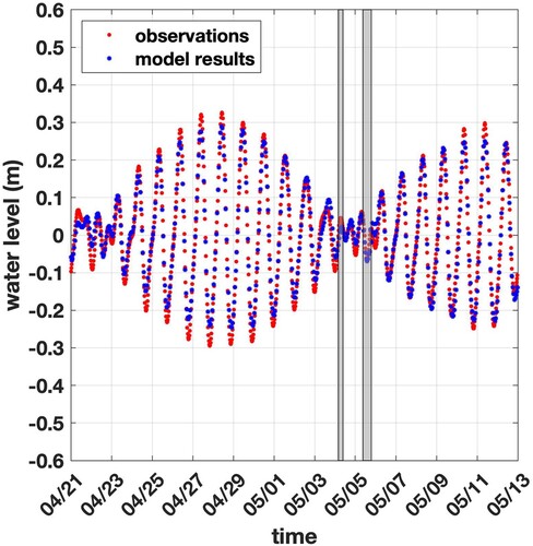
The mean water level (1h-average) relative to the local mean sea level is well predicted, although occasionally, the model underestimates the maxima and minima as much as 0.03-0.05 m (Figure 5) with the skill score as 0.99, the bias as 0.001 m, and the RMSE as 0.029 m.

Figure 5. Water level comparison between model results in blue and hourly averaged water level in red from the shallow quadpod location. The water level is referenced to the local mean sea level. The periods highlighted in gray represent the two periods of sediment accretion at the shallow quadpod location and correspond to the first and second cold front passages.

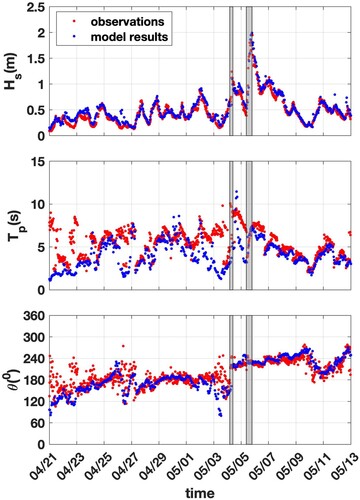
The significant wave height (Hs) and mean wave direction (θ) are well predicted (Figure 6a and c) with the skill score as 0.951, the bias as 0.062 m, the RMAE as 0.028, and the RMSE as 0.134 m for the significant wave height. Applying the RMAE criteria (Table 1), the model performance for Hs is considered ‘excellent.’ However, the wave peak period (Tp) is not well predicted. The model only qualitatively predicts the variation pattern of Tp qualitatively with underestimation in some periods, as illustrated in Figure 6b. The differences between modelled and observed values may be caused by imperfect boundary conditions or unmodeled physical processes.

Figure 6. Comparison of significant wave height (Hs), wave peak period (Tp), and mean wave direction (θ) between model results in blue and observations in red from the shallow quadpod location. The mean wave direction is reported as coming from. The periods highlighted in gray represent the two periods of sediment accretion at the shallow quadpod location and correspond to the first and second cold front passages.

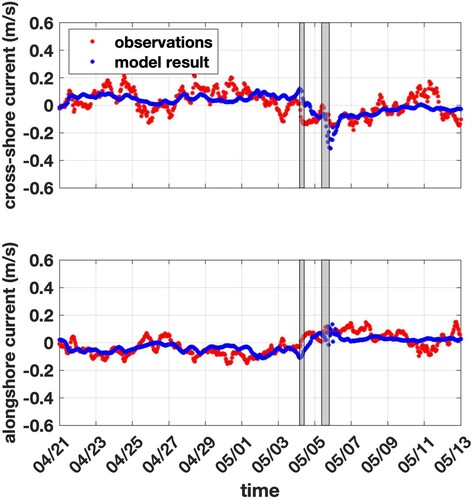
Modelled and observed hourly depth-averaged cross-shore and along-shore currents are determined by rotating the currents 155^o clockwise from north to align with the shoreline (Figure 7). The cross-shore component is represented by positive values when the flow moves onshore and negative values when the flow moves offshore (Figure 7a). The along-shore component is defined by positive values when the flow moves eastward and negative values when the flow moves westward (Figure 7b). The quality of the current speed prediction is represented by the skill score as 0.487, the bias as −0.033 m/s, the RMAE as 0.447, and the RMSE as 0.071 m/s. The bias and RMSE are within limits established in Table 2. The model performance is ‘reasonable’ considering the RMAE criteria (Table 1).

Figure 7. Comparison of cross-shore and alongshore current between model results (in blue) and hourly average currents (in red) observed at the shallow quadpod location. Positive (negative) values of current denote onshore (offshore) flow for the cross-shore component and eastward (westward) flow for the along-shore component. The periods highlighted in gray represent the two periods of sediment accretion at the shallow quadpod location and correspond to the first and second cold front passages.

4.4. Morphological changes

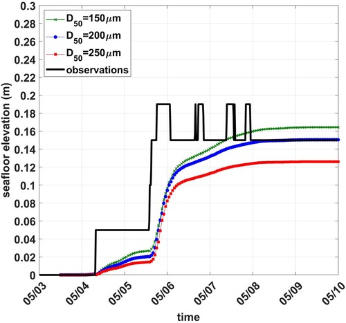
Let $\eta (x,y,t)$ be the model predicted seafloor elevation with (x, y) the cross-shore and alongshore coordinates. Figure 8 shows the model-observation inter-comparison of the seafloor elevation at the shallow quadpod location (x_s, y_s) for the period between 3 and 10 May with different median grain sizes in the model. The black curve represents the time evolution of the seafloor elevation identified from the PC-ADP maximum backscatter. Considering that more than 79% of the sediment samples collected during the TREX13 experiment are classified as fine sand (Calantoni et al., 2014), the morphological module is simulated with three median grain sizes D₅₀ (150μm, 200μm, 250μm) with D₅₀ = 200μm agrees most with the observation. The BSS is computed as 0.913, which is considered as ‘excellent performance’ according to the criteria described in Table 3.

Figure 8. Sediment accretion time series at the shallow quadpod location. The black line indicates the observed seafloor elevation measured from the PC-ADP maximum backscatter. The green, blue, and red lines represent the model output for sediment accretion with different grain sizes.

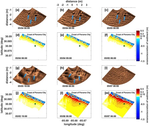
Figure 9 shows the time evolution of sector scanning sonar images and model predicted sediment erosion/accretion at the shallow quadpod location under the two consecutive cold front passages. All sonar images are averaged in a time window of 4 h centred on the date/time displayed in each image to reduce the noise. Before the passage of the first cold front on 4 May 0600 (Figure 9a), the sonar image shows sand ripples and three surrogate munitions highlighted by the blue arrows. On 4 May 0900 (Figure 9b), the incoming swell associated with the first front stirred up the bottom and increased the sediment transport. After the passage of the first cold front on 5 May 0600, the sonar image displays munitions on the seafloor and indicates that the sediment accretion is not sufficient to burial the munitions (Figure 9c). The model prediction of the sediment erosion/accretion before (4 May 0600, Figure 9d), during (4 May 0900, Figure 9e), and after (5 May 0600, Figure 9f) the passage of the first cold front agrees well with observations as minimal sedimentation at the shallow quadpod location represented by the green dot (Figure 9f). The duration of the second cold front is longer than the first front, which leads to more influence on the seafloor. During the second cold front passage on 5 May 1900 and 6 May 0600 (Figure 9g and h), the bedform changed dramatically and the sand partially covered the munitions. Eventually, the munitions were completely buried by 7 May 0600 (Figure 9i). On 8 May, all munitions near the shallow quadpod location were recovered during a maintenance dive, confirming the munitions were buried and not carried by the flow. The morphological module predicts quick sedimentation near the shallow quadpod location due to the second cold front passage (Figure 9j, l, and m), in accordance with the observations.

Figure 9. Sector scanning sonar images and model predicted seafloor elevation η(x, y, t) for sediment erosion/accretion and on 4 May 0600 (a and d), 4 May at 0900 (b and e), 5 May 0600 (c and f), 5 May 1900 (g and j), 6 May 0600 (h and l), and 7 May 0600 (I and m). Sonar images show three munitions (highlighted by the blue arrows) near the shallow quadpod location. Model output covers the detailed domain, with the shallow quadpod location represented by the green dot.

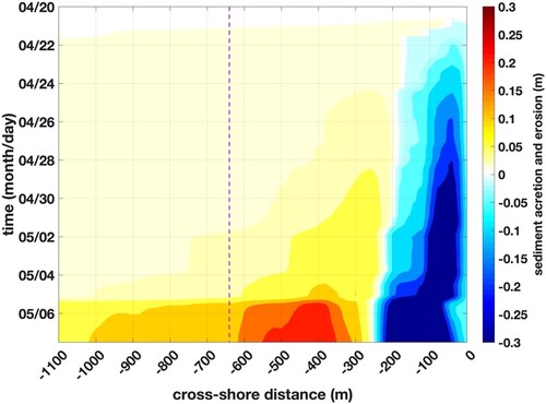
Let $\hat{\eta }(x,t)$ be the alongshore averaged $\eta (x,y,t)$ to show the temporal and cross-shore variability (Figure 10), i.e. the time evolution of the cross-shore erosion/accretion. The basic feature is the nearshore (within 250 m to the coast) erosion and offshore (more than 250 m from the coast) accretion. After the first front passage on May 4 0900, the nearshore erosion reaches a maximum around −0.30 m, and the offshore accretion varies between 0.01 and 0.09 m. During the second front passage from 5 May 1900–6 May 0600, the nearshore erosion increases to −0.45 m and the offshore accretion enhances between 0.09 and 0.25 m. The maximum sedimentation (area in red on Figure 10) is rapidly formed by the end of 5 May between 350 and 550 m offshore.

Figure 10. Temporal and cross-shore variability of $\hat{\eta }(x,t)$ between 20 April and 08 May 2013. The magenta dashed line indicates the cross-shore distance to the shallow quadpod location.

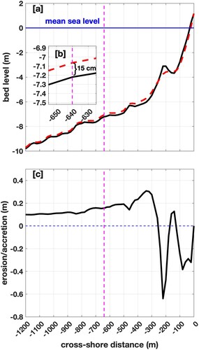
Figure 11 presents the model predicted cross-shore bed level profile through the shallow quadpod location before and after the passage of two consecutive cold fronts (Figure 11a). Inlaid in the figure is a zoomed-in region at the shallow quadpod location showing 15 cm of sediment accretion (Figure 11b). The model predicts the peak sediment erosion (−64 cm) and accretion (30 cm) occurred 220 and 340 m from the shore, respectively. The sediment accretion layer extends in the offshore direction with decreasing thickness as the distance from the shoreline increases. This blanket of 10-20 cm of accretion extends from 500–1200 m from the coastline (Figure 11c).

Figure 11. Development of the cross-shore bed level profile. (a) The black line represents the bed level before the passage of two consecutive cold fronts, and the red line is the result of the model simulation denoting the bed level after the consecutive cold front passages. (b) Zooming around the shallow quadpod location to show the 15 cm of sediment accretion. (c) The cross-shore erosion/accretion of sediment along the profile containing the shallow quadpod location. The magenta dashed line indicates the cross-shore distance to the shallow quadpod location.

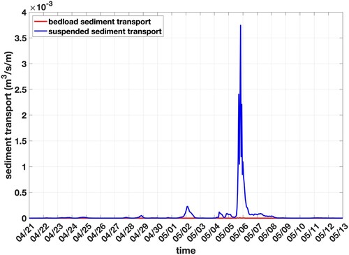
Tidal currents can greatly influence sediment transport, particularly in areas with a large tidal range. However, during the field experiment, the small tidal range varying between 0.5 m (spring tide cycle) and 0.2 m (neap tide cycle) results in weak tidal currents, especially in the neap tide cycle. To verify the influence of tidal current on sediment transport, a model simulation without waves but with tidal forcing (not shown here) revealed minimal sediment transport and no evident morphological changes in the study area, suggesting that tides play a passive role in short-term (i.e. few weeks) sediment transport and morphological changes. In contrast, the model simulation, including waves, presented peaks of suspended sediment transport at the shallow quadpod location (Figure 12) during the wave events, implying that waves play the primary role in sediment transport and morphological changes. Furthermore, the model results indicate that suspended sediment transport is predominant, and the bedload sediment transport is minimal.

Figure 12. Model results for suspended (blue line) and bedload (in red) sediment transport at the shallow quadpod location.

5. Conclusion

Interaction between waves and the seafloor during two consecutive atmospheric cold front passages over a lower-energetic area is studied using observations from the TREX13 experiment off the coast of Panama City, Florida, in April-May 2013 and the open-source modelling system Delft3D. The model accurately simulates waves, currents, and morphological changes, including a rapid increase in seafloor elevation after two consecutive cold fronts observed from the PC-ADP at the shallow quadpod (7.5 m water depth). The model simulation indicates that erosion nearshore and sediment accretion offshore starting 250 m from the coast are enhanced during the passage of the cold fronts, suggesting waves have the primary role in driving the observed morphological changes. In addition, the sediment accretion coincided with the burial of surrogate munitions observed with sonar imagery at the shallow quadpod location, which adds to the contributions of Klammler et al. (2021), who pointed out the occurrence of sediment liquefaction at the exact location during the field experiment, by indicating that sediment accretion also contributes to the observed morphological changes and munition burial. The sediment liquefaction is not included in the Delft3D morphological module and will be investigated in future studies. The results presented in this work demonstrate the possibility of using the model in the risk assessment and cost reduction related to remediation efforts through quality identification of morphological change of seafloor for the prediction of mobility and burial of underwater munitions.

Acknowledgments

The authors would like to thank Dr. Joseph Calantoni at the Naval Research Laboratory at the Stennis Space Centre for providing the TREX13 data.

Disclosure statement

No potential conflict of interest was reported by the author(s).

Additional information

Funding

This research was funded by the Strategic Environmental Research and Development Program (SERDP) with the funding document numbers of W74RDV908l8446 and W74RDV00801666.

References

- Battjes JA, Janssen JPFM. 1978. Energy loss and set-up due to breaking random waves. Proceedings of the 16th international conference on coastal engineering. Am Soc of Civ Eng. 1:569–587.
- Bennett R. 2000. Mine Burial Prediction Workshop Report and Recommendations. SEAPROBE, Inc. Technical Report Number SI-0000-03.
- Booij N, Ris RC, Holthuijsen LH. 1999. A third-generation wave model for coastal regions: 1. model description and validation. J Geophys Res. 104:7649–7666.
- Bunya S, Dietrich JC, Westerink JJ, Ebersole BA, Smith JM, Atkinson JH, Jensen R, Resio DT, Luettich RA, Dawson C, Cardone VJ. 2010. A high-resolution coupled riverine flow, tide, wind, wind wave, and storm surge model for southern louisiana and Mississippi. part I: Model development and validation. Mon Wea Rev. 138:345–377.
- Calantoni J, Staples T, Sheremet A. 2014. Long time series measurements of munitions mobility in wave-current boundary layer. Report SERDP Project Number 2320. https://www.serdp-estcp.org/Program-Areas/Munitions-Response/Munitions-Underwater/MR-2320/(language)/eng-US.
- Callaghan DP, Nielsen P, Ranasinghe R. 2008. Statistical simulation of wave climate and extreme beach erosion. Coastal Eng. 55:375–390.
- Chu PC. 2009. Mine impact burial prediction from one to three dimensions. Appl Mech Rev 62:1–25.
- Chu PC, Fan CW. 2005. Pseudo-cylinder parameterization for mine impact burial prediction. J Fluids Eng. 127:1515–1520.
- Chu PC, Fan CW. 2006. Prediction of falling cylinder through air-water-sediment columns. ASME J Appl Mechanics. 73:300–314.
- Chu PC, Fan CW. 2022. User’s Guide: Underwater Munition Scour Burial (UnMUSB) Model. Technical Report, NPS-OC-22-002, Naval Postgraduate School, Monterey, CA, USA., 1-70 (available at https://calhoun.nps.edu/bitstream/handle/10945/69292/NPS-OC-22-002.pdf?sequence=1&isAllowed=y).
- Chu PC, Fan CW, Calantoni J, Sheremet A. 2022. Prediction of mobility and burial of objects on sandy seafloor. IEEE J Oceanic Eng. 47(1):111–125.
- Chu PC, Fan CW, Evans AD, Gilles AF. 2004. Triple coordinate transforms for prediction of falling cylinder through the water column. J Appl Mech. 71:292–298.
- Chu PC, Gilles AF, Fan CW. 2005. Experiment of falling cylinder through the water column. Exp Therm Fluid Sci. 29:555–568.
- Chu PC, Pauly P, Haeger SD, Ward M. 2006. Wind and tidal effects on chemical spill in St andrew Bay system. Coastal Environ Water Quality. 1:47–68.
- Chu PC, Pessanha VS, Fan CW, Calantoni J. 2021. Coupled Delft3D-object model to predict mobility of munition on sandy seafloor. Fluids. 6(9):330.
- Deltares. 2019a. Delft3D-Flow—Simulation of multi-dimensional hydrodynamic flows and transport phenomena, including sediments, User Manual. https://content.oss.deltares.nl/delft3d/manuals/Delft3D-FLOW_User_Manual.pdf.
- Deltares. 2019b. Delft3D-Wave—Simulation of short-crested waves with SWAN, User Manual. https://content.oss.deltares.nl/delft3d/manuals/Delft3D-WAVE_User_Manual.
- DiMego GJ, Bosart LF, Endersen GW. 1976. An examination of the frequency and mean conditions surrounding frontal incursions into the Gulf of Mexico and Caribbean Sea. Mon Weather Rev. 104:709–718.
- ECMWF. 2019. ERA5 Reanalysis (0.25 Degree Latitude-Longitude Grid), Research Data Archive at the National Center for Atmospheric Research, Computational and Information Systems Laboratory, Boulder, CO, accessed on 3 July 2019, https://rda.ucar.edu/datasets/ds633.0.
- Farrar PD, Borgman LE, Glover LB, Reinhard RD, Pope J, Swain A, Ebersole BA. 1994. Storm impact assessment for beaches at Panama City, Florida. U.S. Army Engineer Waterways Experiment Station. Report CERC-94-11. http://citeseerx.ist.psu.edu/viewdoc/download?doi=10.1.1.371.2181&rep=rep1&type=pdf.
- Ferreira Ó. 2005. Storm groups versus extreme single storms: predicted erosion and management consequences. J Coast Res. 42:155–161.
- Guo B, Subrahmanyam MV, Li C. 2020. Waves on louisiana continental shelf influenced by atmospheric fronts. Sci Rep. 10:272.
- Hasselmann K. 1974. On the spectral dissipation of ocean waves due to white capping. Boundary-Layer Meteor. 6:107–127.
- Klammler, H., Penko, A.M., Staples, T., Sheremet, A. and Calantoni, J. (2021). Observations and modeling of wave-induced burial and sediment entrainment: likely importance of degree of liquefaction. J Geophys Res Oceans, 126(8). https://doi.org/10.1029/2021JC017378.
- Komar PD. 1976. Beach processes and sedimentation. USA: Prentice Hall, pp. 16–33.
- Lee GH, Nicholls RJ, Birkemeier WA. 1998. Storm-driven variability of the beach-nearshore profile at duck, north carolina, USA, 1981–1991. Mar Geol. 148:163–177.
- Lesser GR, Roelvink JA, van Kester JATM, Stelling GS. 2004. Development and validation of a three-dimensional morphological model. Coastal Eng. 51:883–915.
- Morton RA, Gibeaut JC, Paine JG. 1995. Meso-scale transfer of sand during and after storms: implications for prediction of shoreline movement. Mar Geol. 126:161–179.
- NOAA/NGDC. 2010. Northern Gulf 1 arc-second MHW Coast Digital Elevation Model, accessed on 17 December 2018, https://catalog.data.gov/dataset/northern-gulf-coast-digital-elevation-model156ed.
- NOAA/WPC. 2020. Weather Prediction Center’s Surface Analysis Archive, accessed on 10 August 2020, https://www.wpc.ncep.noaa.gov/archives/web_pages/sfc/.
- Pessanha VS. 2019. Modeling of Morphological Responses to a Storm Event During TREX13. Master’s Thesis, Naval Postgraduate School, Monterey, CA, U.S.A., December 2019.
- Plant NG, Long JW, Dalyander PS, Thompson DM, Raabe EA. 2013. Application of a hydrodynamic and sediment transport model for guidance of response efforts related to the Deepwater Horizon oil spill in the northern Gulf of Mexico along the coast of Alabama and Florida, U.S, Geological Survey, Report number 2012–1234. http://pubs.usgs.gov/of/2012/1234/.
- Roelvink D, Reniers A. 2012. A guide to modeling coastal morphology. Singapure: World Science Publishing Co. Pte. Ltd, pp. 274.
- Roelvink D, Walstra DJ. 2004. Keeping it simple by using complex models. Adv Hydro-Science Eng. 6:1–11.
- SERDP-ESTCP. 2010. Munitions in the Underwater Environment: State of the Science and Knowledge Gaps. https://www.serdp-estcp.org/Featured-Initiatives/Munitions-Response-Initiatives/Munitions-in-the-Underwater-Environment/White-Paper-Munitions-in-the-Underwater-Environment.
- Taiani L, Benedet L, Silveira L, Keehn S, Sharp N, Bonanata R. 2012. : Sand borrow area design refinement to reduce morphological impacts: A case study of Panama City Beach, Florida, USA. Coastal Eng Proceedings. 1:103–113.
- Van Rijn LC. 2013. Erosion of Coastal dunes Due to storms. Blokzijl, The Netherlands: Leovanrijn-Sediment, pp. 1–18.
- Van Rijn LC, Walstra D, Grasmeijer B, Sutherland J, Pan S, Sierra J. 2003. The predictability of cross-shore bed evolution of sandy beaches at the time scale of storms and seasons using process-based profile models. Coastal Eng. 47:295–327.
- Vousdoukas MI, Almeida LP, Ferreira Ó. 2012. Beach erosion and recovery during consecutive storms at a steep-sloping, meso-tidal beach. Earth Surf Process. Landforms. 37:583–593.
- Williams J, Esteves L. 2017. Guidance on setup, calibration, and validation of hydrodynamic, wave, and sediment models for shelf seas and estuaries. Adv Civil Eng. 2017:1–25.
- Willmott CJ. 1981. On the validation of models. Physical Geography. 2:184–194.