The contribution of livestock to climate change mitigation: a perspective from a low-income country

Abstract

The livestock sector in low- and middle-income countries could contribute significantly to reduce the rate of growth and/or the level of greenhouse gas (GHG) emissions required to achieve the 1.5 °C target of the Paris Agreement. Yet, the sector is also expected to contribute to food and income security in these countries. Using an extensive dataset on the Ethiopian livestock sector, we assessed the potential of selected interventions to increase supply of animal source protein (ASP) and reduce GHG emissions intensity or absolute emissions at national level. The business as usual (BAU) scenario was modelled by extrapolating the historical trends observed during the base years (i.e. 2010 – 2020) to the period between 2021 and 2030. Four scenarios were modelled including structural changes in cattle herd (S1) and chicken flock (S3) composition, increased milk yields of dairy cattle (S2), and a combination of all strategies (S4). We found that the total ASP produced and supplied per capita, as well as total GHG emissions increased between 2021 and 2030 across all scenarios while emission intensities per unit ASP produced decreased. However, by 2030, the total GHG emissions in S1 (i.e. 146.7 MtCO₂e) were lower than in the BAU scenario (i.e. 149.0 MtCO₂e) while the total ASP supplied per capita was higher in the former (i.e. 6.84 kg) than the latter (i.e. 6.24 kg). These findings suggest that structural changes at herd level could reduce total GHG emissions and concomitantly increase ASP supply. Therefore, structural transformation could be a highly relevant policy option for low- and middle- income countries, where the livestock sector must address multiple goals including food and income security, and global climate commitments.

Keywords:

• Greenhouse gas emissions
• livestock development strategies
• global climate objectives
• animal source protein
• low- and middle-income countries

Introduction

Greenhouse gases (GHG) are the main drivers of global climate change. Livestock production systems account for about 14.5% of all anthropogenic GHG and 70% of all emissions from agriculture, forestry, and other land use [1,2]. The main GHG from livestock include methane (CH₄) and nitrous oxide (N₂O), with the former accounting for more than 70% of livestock emissions, making CH₄ the most important non-CO₂ GHG from the agricultural sector [3,4]. Methane is a short-lived GHG that contributes to the formation of tropospheric ozone, thereby negatively affecting human health and agricultural productivity [4–6]. Over the first 20 years after being released into the atmosphere, CH₄ has a global warming potential (GWP) that is 84 times greater than that of CO₂, resulting in significant short-term effects on climate change [7]. Also, CH₄ is responsible for at least 25% of the global warming experienced worldwide [4]. Ruminants are the main emitters of CH₄, via enteric fermentation and from manure. Therefore, livestock remains a key focus of attention for addressing climate change.

While global CH₄ and N₂O emissions from livestock have increased by about 32% over the last decade, the emission trends differ between low- and middle- income countries and high income countries [8]. Total livestock GHG emissions from high income countries have remained stable while there has been an increasing trend in emissions from low- and middle- income countries (Figure 1). This increasing trend in emissions is driven by increases in population, urbanization and per capita incomes, and a concomitant demand for animal source protein (ASP) [9,10].

Figure 1. Trends in livestock greenhouse gases (methane and nitrous oxide expressed as CO₂ equivalent) emissions during the period from 2005 to 2019 for low- and middle- income countries. (Data source: [8]).

It is projected that in the decades to 2050, the largest increases in demand for ASP and thus livestock GHG emissions will be in Sub-Saharan Africa (SSA), where population and urbanization rates could almost double [10,11]. Growth in the livestock sub-sector may present opportunities for millions of smallholder farmers in the region, but could also aggravate climate change, air and water pollution, loss of biodiversity, and health risks associated with consumption of ASP [9, 12].

Trends in livestock emissions from low- and middle- income countries have an important bearing on the global potential to achieve the 1.5 °C target of the Paris Agreement [13]. As such, several low- and middle- income countries have included the livestock sector in their nationally determined contributions (NDCs) submitted to United Nations Framework Convention on Climate Change [14]. On one hand, livestock production systems in these nations are targeted to reduce the rate of growth and/or the level of emissions [15]. On the other hand, the sector is expected to increasingly contribute towards sustainable development and poverty alleviation by contributing to food and income security, and providing ecosystem services [16,17]. While many strategies that reduce GHG emissions at animal level are known, practically reconciling environmental impacts from livestock production and sustainable national development objectives remains a challenge [18–20]. Current productivity levels are low in most low- and middle- income countries while the demand for ASP is rising. Hence, increasing production efficiency has been identified as one strategy to balance national development objectives with reducing the environmental impacts of livestock in low- and middle- income countries [21–23]. Production efficiency may be improved by increasing animal and herd productivity or structural changes in the sector via a more rapid growth of animal numbers in higher productivity systems, and/or a more rapid growth in populations of low-emitting species. However, there has also been criticism that improving production efficiency and reducing emission intensity may not lead to the reductions in absolute emissions required to meet the 1.5 degree target [24].

Taking the example of Ethiopia, the present study assessed the potential of livestock development strategies to increase supply of ASP and reduce GHG emissions intensity or absolute emissions at national level in a low-income country in SSA. Ethiopia was selected as case study because it possesses the largest livestock herd in Africa, with about 70 million cattle [25]. In addition, Ethiopia’s national commitments on climate change mitigation give high priority to the livestock sector, as shown in their updated NDC [26]. First, we summarized and presented a methodology for estimating the emission intensity per unit ASP. Next, using an extensive data set on the Ethiopian livestock sector, we assessed the potential of selected development strategies to increase supply of ASP and reduce GHG emissions intensity or absolute emissions. In the discussion section, we assess our findings in the context of international discussions on the role of livestock in climate change mitigation.

Materials and methods

Emissions intensity methodology

Several studies have presented methods for estimating the emission intensity of livestock products (e.g. 23]. Here, we used a simple approach modified after [27], to accommodate the main forms of ASP found in the main livestock production systems in Ethiopia. The common denominator of all ASPs is protein and GHG emission intensities were expressed per unit ASP output as shown in Equation 1(1) $$\text{GHG}\mathrm{ }\text{intensity}\mathrm{X}=\frac{\text{total}\mathrm{ }\text{GHG}\mathrm{ }\text{emissions}}{\text{total}\mathrm{ }\text{protein}\text{output},\mathrm{X}}$$(1) : (1) $$\text{GHG}\mathrm{ }\text{intensity}\mathrm{X}=\frac{\text{total}\mathrm{ }\text{GHG}\mathrm{ }\text{emissions}}{\text{total}\mathrm{ }\text{protein}\text{output},\mathrm{X}}$$(1) where GHG intensity_x is the greenhouse gas emission intensity per unit protein produced from the livestock sector in year X (kg CO₂e/kg protein), total GHG emissions the sum of all GHGs emitted by livestock in year X (MtCO₂e/year), and total protein_output,x the total protein output from all ASP sources, including eggs, meat, and milk produced in year X (Mt protein/year).

Total GHG emissions from each livestock species and production system were estimated using the Tier 2 approach of the IPCC guidelines for different livestock species. Total GHG emissions (MtCO₂e/year) were estimated for each species and production system as the sum of emissions from different sources (Equation 2(2) $$\text{GHG}\mathrm{ }\text{emission}\mathrm{S}={\sum }_{\mathrm{S}}\mathrm{(}[\mathrm{(}{\text{EF}\_\text{CH}4}_{\mathrm{S},\mathrm{X}}+{\text{MM}\_\text{CH}4}_{\mathrm{S},\mathrm{X}}\text{) }\text{x }{\text{GWP}}_{\text{CH}4}]+[\left({\text{MM}\_\mathrm{N}2\mathrm{O}}_{\mathrm{S},\mathrm{X}}+{\text{PRP}\_\mathrm{N}2\mathrm{O}}_{\mathrm{S},\mathrm{X}}\right)\mathrm{x}\mathrm{ }{\text{GWP}}_{\mathrm{N}20}\mathrm{])}$$(2) ). (2) $$\text{GHG}\mathrm{ }\text{emission}\mathrm{S}={\sum }_{\mathrm{S}}\mathrm{(}[\mathrm{(}{\text{EF}\_\text{CH}4}_{\mathrm{S},\mathrm{X}}+{\text{MM}\_\text{CH}4}_{\mathrm{S},\mathrm{X}}\text{) }\text{x }{\text{GWP}}_{\text{CH}4}]+[\left({\text{MM}\_\mathrm{N}2\mathrm{O}}_{\mathrm{S},\mathrm{X}}+{\text{PRP}\_\mathrm{N}2\mathrm{O}}_{\mathrm{S},\mathrm{X}}\right)\mathrm{x}\mathrm{ }{\text{GWP}}_{\mathrm{N}20}\mathrm{])}$$(2) where EF_CH4 is the methane emitted via enteric fermentation by all animal species (ruminants only and not monogastrics e.g. poultry) in production system S in year X, MM_CH4 the methane emitted via manure management by all animals in production system S in year X, GWP_CH4 the global warming potential of methane, MM_N2O the sum of direct and indirect nitrous oxide emissions via manure management by all animals in production system S in year X, PRP_N2O the sum of direct and indirect nitrous oxide emissions from dung and urine deposited on pasture by all animals in production system S in year X, and GWP_N2O the global warming potential of nitrous oxide. Emissions were converted from Gg to Mt by dividing by 1000. In contrast to full lifecycle assessments (e.g. 27], the emission sources included in our study included only direct livestock emissions from enteric fermentation and manure.

The total output of ASP was estimated as (Equation 3(3) $$\text{Total}\mathrm{ }\text{Protein}\text{output},\mathrm{X}={\text{PO}}_{\text{meat},\mathrm{ }\mathrm{X}}+{\text{PO}}_{\text{milk},\mathrm{X}}+{\text{PO}}_{\text{eggs},\mathrm{X}}$$(3) ): (3) $$\text{Total}\mathrm{ }\text{Protein}\text{output},\mathrm{X}={\text{PO}}_{\text{meat},\mathrm{ }\mathrm{X}}+{\text{PO}}_{\text{milk},\mathrm{X}}+{\text{PO}}_{\text{eggs},\mathrm{X}}$$(3) where PO_meat,X, PO_milk,X, and PO_eggs,X are the total protein output (Mt protein) from meat, milk, and eggs, respectively, from all livestock species and production systems in year X.

The total protein output from meat in year X was estimated for all animal cohorts following [28] as (Equation 4(4) $${\text{PO}}_{\text{meat},\mathrm{ }\mathrm{X}}=\frac{{\sum }_{\mathrm{s}}{\mathrm{(}\mathrm{n}\_\text{off}}_{\mathrm{S},\mathrm{X}}\text{ x }{\text{LW}}_{\mathrm{S},\mathrm{X}}\text{ x }\frac{{\text{DP}}_{\mathrm{S}}}{100}\text{) }\text{x}\left(\frac{{\text{BFM}}_{\mathrm{S}}\text{ x }{\text{meat}\_\text{prot}}_{\mathrm{S}}}{100}\right)}{1000000}$$(4) ): (4) $${\text{PO}}_{\text{meat},\mathrm{ }\mathrm{X}}=\frac{{\sum }_{\mathrm{s}}{\mathrm{(}\mathrm{n}\_\text{off}}_{\mathrm{S},\mathrm{X}}\text{ x }{\text{LW}}_{\mathrm{S},\mathrm{X}}\text{ x }\frac{{\text{DP}}_{\mathrm{S}}}{100}\text{) }\text{x}\left(\frac{{\text{BFM}}_{\mathrm{S}}\text{ x }{\text{meat}\_\text{prot}}_{\mathrm{S}}}{100}\right)}{1000000}$$(4) where n_off_S,X is the total number of animals slaughtered (n) by species in production system S in year X, LW_S,X the average live weight (kg) of animals slaughtered in production system S in year X, DP_S the dressing percentage for animals by species in production system S, BFM_S the bone-free-meat percentage (ratio of bone free meat to cold carcass weight) for animals by species in production system S, meat_prot_S the mean protein content (g/100g) in the meat of the animals by species in production system S, and 1,000,000 the conversion factor from kg to Mt.

The total protein output from milk in year x was estimated as (Equation 5(5) $${\text{PO}}_{\text{milk},\mathrm{ }\mathrm{x}}=\frac{{\sum }_{\mathrm{s}}\mathrm{(}{\mathrm{(}\text{lact}\_\text{animals}}_{\mathrm{s},\mathrm{x}}\text{ x }{\text{FPCM}}_{\mathrm{s},\mathrm{x}}\text{) x (}\frac{{\text{prot}}_{\text{milk}}}{100}\mathrm{)}\mathrm{)}}{1000000}$$(5) ): (5) $${\text{PO}}_{\text{milk},\mathrm{ }\mathrm{x}}=\frac{{\sum }_{\mathrm{s}}\mathrm{(}{\mathrm{(}\text{lact}\_\text{animals}}_{\mathrm{s},\mathrm{x}}\text{ x }{\text{FPCM}}_{\mathrm{s},\mathrm{x}}\text{) x (}\frac{{\text{prot}}_{\text{milk}}}{100}\mathrm{)}\mathrm{)}}{1000000}$$(5) where lact_animals_s,x is the total number of lactating animals (n) by species in production system S in year X, FPCM_s,x the mean annual milk yield (kg) corrected for fat and protein per lactating animal by species in production system S in year X, prot_milk the mean protein content of milk (g/100g) by species and production system, and 1,000,000 the conversion factor from kg to Mt. The mean annual milk yields of cows and small ruminants were corrected for fat and protein following Equations 6(6) $$\text{FPCM}=\text{MY}\text{ x (}0.337+\mathrm{(}0.116\text{ x }\text{MF}\mathrm{)}+\mathrm{(}0.06\text{ x }\text{MP}\mathrm{)}\mathrm{)}$$(6) and 7(7) $$\text{FPCM}=\text{MY}\text{ x (}0.25+\mathrm{(}0.085\text{ x }\text{MF}\mathrm{)}+\mathrm{(}0.035\text{ x }\text{MP}\mathrm{)}\mathrm{)}$$(7) , respectively [27, 29]. (6) $$\text{FPCM}=\text{MY}\text{ x (}0.337+\mathrm{(}0.116\text{ x }\text{MF}\mathrm{)}+\mathrm{(}0.06\text{ x }\text{MP}\mathrm{)}\mathrm{)}$$(6) (7) $$\text{FPCM}=\text{MY}\text{ x (}0.25+\mathrm{(}0.085\text{ x }\text{MF}\mathrm{)}+\mathrm{(}0.035\text{ x }\text{MP}\mathrm{)}\mathrm{)}$$(7) where MY is the mean annual milk yield (kg) per lactating animal, MF the milk fat content (g/100g), and MP the milk protein content (g/100g).

Total protein output from eggs was estimated as (Equation 8(8) $${\text{PO}}_{\text{eggs},\mathrm{ }\mathrm{x}}=\frac{{\sum }_{\mathrm{s}}{\mathrm{(}\text{chicken}\_\text{pop}}_{\mathrm{s},\mathrm{x}}\text{ x }{\text{eggs}\_\text{laid}}_{\mathrm{s},\mathrm{x}}\text{ x }{\text{egg}\_\text{wght}}_{\mathrm{s},\mathrm{x}}\text{ x }{\text{prot}}_{\text{egg}}\mathrm{)}}{1000000}$$(8) ): (8) $${\text{PO}}_{\text{eggs},\mathrm{ }\mathrm{x}}=\frac{{\sum }_{\mathrm{s}}{\mathrm{(}\text{chicken}\_\text{pop}}_{\mathrm{s},\mathrm{x}}\text{ x }{\text{eggs}\_\text{laid}}_{\mathrm{s},\mathrm{x}}\text{ x }{\text{egg}\_\text{wght}}_{\mathrm{s},\mathrm{x}}\text{ x }{\text{prot}}_{\text{egg}}\mathrm{)}}{1000000}$$(8) where chicken_pop_s,x is the total population of hens (n) in production system S laying eggs for human consumption only in year X, eggs_laid_S,X the total number of eggs laid (n) per hen for human consumption in production system S in year X, egg_wght_S,X the mean egg weight from production system S in year X, prot_egg the mean protein fraction in eggs, and 1,000,000 the conversion factor from kg to Mt.

Case study on the Ethiopian livestock sector

Ethiopia is a landlocked nation in the Horn of Africa, and the second most populated country on the continent [11]. The country’s economy is mainly driven by tourism and agriculture, with the latter employing over 75% of the active labor force [26]. The Ethiopian livestock sector is an important pillar of the nation’s economy, accounting for 18.7% of national GDP and up to 19% of foreign exchange earnings [30]. The livestock sector is also responsible for over 60% of all agricultural GHG emissions, with cattle, sheep, and goats emitting 107 Mt CO₂e in 2018 [31].

The country recently updated its NDC and integrated a sector-wise plan for climate change adaptation and mitigation of GHG emissions within its national Ten Year Development plan (10YDP) that runs from 2020 to 2030 [26]. The NDC projects that emissions from the livestock sector would reach 194.8 Mt CO₂e by 2030 if no changes are made to current production practices (i.e. business-as-usual [BAU]). The NDC defined policy interventions to achieve a 7.6% (i.e. −14.8 Mt CO₂e) reduction in emissions from the sector by 2030 relative to BAU projections, conditional on receiving international financial support to supplement Ethiopia’s own resources [26].

In the next section, first we calculated an emission intensity BAU scenario for Ethiopia using data from 2010 to 2020. Next, we projected the livestock population and productivity from 2021 to 2030 under different scenarios to evaluate the impact of different livestock development strategies on emission intensities and per capita ASP supply.

Emission intensity baseline for Ethiopia

A three-step approach was employed to estimate emission intensity for the base period (i.e. 2010 to 2020) per Mt protein from cattle, sheep, goats, and chickens in Ethiopia. First, we assembled data on animal populations for different production systems, and their productive and reproductive performances. The data for 2010 to 2018 were reported¹ by production system in [31] and have been adopted for the present study (Table 1). For 2019 and 2020, the population, productive and reproductive performance, and offtake data were extracted from the annual agricultural sample survey reports of the Ethiopian Central Statistical Agency [25, 33] and analyzed using the same methods as in [31].

Table 1. Livestock species, production systems and livestock categories considered for estimating greenhouse gas emissions in Ethiopia.

Species	Production systems	Livestock types
Cattle	Mixed crop-livestock	Dual purpose cattle
	Pastoral and agropastoral	Dual purpose cattle
	Smallholder intensive	Dairy cattle
	Commercial	Dairy cattle
Sheep and goats	Mixed crop-livestock	Hybrid and exotic
	Pastoral and agropastoral	Indigenous
Chicken*	Low productivity	Indigenous and hybrid chicken
	Average productivity	Exotic chicken
	High productivity	Commercial chicken

* GHG emissions from chickens were not reported in [31]. The production systems shown are based on the categories suggested in the IPCC Guidelines [32] which were aligned with chicken sub-categories reported by the Ethiopian Central Statistical Agency (See Table 4).

Second, we estimated the total annual GHG emissions from cattle, sheep, goats, and chickens in Ethiopia from 2010 to 2020 as the sum of emissions from all sources as shown in Equation 2(2) $$\text{GHG}\mathrm{ }\text{emission}\mathrm{S}={\sum }_{\mathrm{S}}\mathrm{(}[\mathrm{(}{\text{EF}\_\text{CH}4}_{\mathrm{S},\mathrm{X}}+{\text{MM}\_\text{CH}4}_{\mathrm{S},\mathrm{X}}\text{) }\text{x }{\text{GWP}}_{\text{CH}4}]+[\left({\text{MM}\_\mathrm{N}2\mathrm{O}}_{\mathrm{S},\mathrm{X}}+{\text{PRP}\_\mathrm{N}2\mathrm{O}}_{\mathrm{S},\mathrm{X}}\right)\mathrm{x}\mathrm{ }{\text{GWP}}_{\mathrm{N}20}\mathrm{])}$$(2) above. We employed the Tier 2 methodology of the IPCC [34] to estimate emissions from different sources for cattle, sheep, and goats in Ethiopia. When country specific data needed to estimate emission factors for CH₄ and N₂O from manure management for all three species were unavailable, we used default values from IPCC [32] guidelines, similar to [31]. Due to a lack of sufficient data to apply the Tier 2 method, GHG emissions from chickens were estimated using the Tier 1 method [32]. Default values for the parameters required (Table 2) were extracted from the IPCC [32] guidelines for each level of chicken productivity in Ethiopia and applied following Equation 2(2) $$\text{GHG}\mathrm{ }\text{emission}\mathrm{S}={\sum }_{\mathrm{S}}\mathrm{(}[\mathrm{(}{\text{EF}\_\text{CH}4}_{\mathrm{S},\mathrm{X}}+{\text{MM}\_\text{CH}4}_{\mathrm{S},\mathrm{X}}\text{) }\text{x }{\text{GWP}}_{\text{CH}4}]+[\left({\text{MM}\_\mathrm{N}2\mathrm{O}}_{\mathrm{S},\mathrm{X}}+{\text{PRP}\_\mathrm{N}2\mathrm{O}}_{\mathrm{S},\mathrm{X}}\right)\mathrm{x}\mathrm{ }{\text{GWP}}_{\mathrm{N}20}\mathrm{])}$$(2) above to estimate total GHG emissions. To ensure our emission estimates were consistent with those in Ethiopia’s NDC, the present study employed 1, 28, and 265 as the GWP values for CO₂, CH₄ and N₂O, respectively [39].

Table 2. Overview of parameters and default values used to estimate Tier 1 greenhouse gas emissions for chickens in Ethiopia.

Emissions	Parameters	Productivity levels
		Low	Average^35	High
Methane (CH4)	Volatile solids excretion rate (kg/1000 kg animal mass/day) ^36	13.0	12.6	12.3
	Live weight (kg)^37	1.6	1.8	2.0
	Volatile solids excretion (kg/animal/year)^38	7.35	8.16	8.98
	Maximum CH4 producing capacity (m^3 CH4/kg VS)^2	0.24	0.615	0.375
	CH4 conversion factor for manure management system (%) ^23	0.007	0.015	0.227
	Emission factor (kg CH4/head/yr) ^33	0.013	0.075	0.763
Nitrous oxide (N2O)	Nitrogen excretion rate (kg N/1000 kg animal mass/day) ^25	1.44	1.29	1.16
	Emission factor [EF3] from manure management (kg N2O-N/kg N)^22	0.0015	0.0015	0.0015
	Direct N2O emissions from manure management (kg N2O/year)^30	0.0019	0.0019	0.0019

¹ Own defined level to accommodate production systems whose definition lies between low and high productivity. Values for the average productivity level were obtained by averaging the default values for each parameter reported in [32] for low and high chicken productivity systems.

² ([32], Table 10.13 A);.

³ Own data;.

⁴ ([32], Equation 10.22 A);.

⁵ ([32], Table 10.16);.

⁶ ([32], Table 10.17). In low productive systems, 50 % of manure remains on pasture/where chickens scavenge and 50 % is spread daily after removal from the confinement facility, while in high productivity systems, 90 % of the manure produced is stored in pits for 1 month and the remaining 10 % is allowed to accumulate with litter.

⁷ Obtained by multiplying ^4,5 and ⁶ at each productivity level.

⁸ ([32], Table 10.19);.

⁹ ([32], Table 10 A.9). In low productivity systems, 50 % of manure remains on pasture/wherever the chickens scavenge and 50 % is spread daily after removal from the confinement facility, while in high productivity systems, 90 % of the manure produced is stored in pits for 1 month and the remaining 10 % is allowed to accumulate with litter; and.

¹⁰ ([32], Equation 10.25).

Third, we estimated the total protein output from each livestock species according to Equations 3(3) $$\text{Total}\mathrm{ }\text{Protein}\text{output},\mathrm{X}={\text{PO}}_{\text{meat},\mathrm{ }\mathrm{X}}+{\text{PO}}_{\text{milk},\mathrm{X}}+{\text{PO}}_{\text{eggs},\mathrm{X}}$$(3) to 8(8) $${\text{PO}}_{\text{eggs},\mathrm{ }\mathrm{x}}=\frac{{\sum }_{\mathrm{s}}{\mathrm{(}\text{chicken}\_\text{pop}}_{\mathrm{s},\mathrm{x}}\text{ x }{\text{eggs}\_\text{laid}}_{\mathrm{s},\mathrm{x}}\text{ x }{\text{egg}\_\text{wght}}_{\mathrm{s},\mathrm{x}}\text{ x }{\text{prot}}_{\text{egg}}\mathrm{)}}{1000000}$$(8) . The Ethiopian Central Statistical Agency reports the total animal offtake (i.e. sales and slaughtered) by species, breed, sex and geographical zone of production in its annual agricultural sample surveys. Offtake data were extracted from the annual agricultural sample surveys for the period from 2010 to 2020. However, the annual agricultural sample surveys do not cover households in urban and peri-urban areas, or farms owned by companies. Therefore, three assumptions were made to fill data gaps in the animal offtake data:

1. The annual offtake rate on commercial dairy farms was assumed to be 15% of the total population;

2. All cattle kept on smallholder feedlots in the mixed crop-livestock system in each year were assumed to be sold and slaughtered in that year; and

3. All cattle kept on commercial feedlots in the urban and peri-urban areas were assumed to be sold in that year and the total meat output corresponds to the total volume (tonnes) of bovine meat exported.

The total volume of meat exported from Ethiopia was obtained from the International Trade Center (using the sum of the categories ‘0201 – meat of bovine animals, fresh or chilled’ and ‘0202 – meat of bovine animals, frozen’ (https://www.trademap.org/Index.aspx). The number of animals exported was calculated as: (9) $$\mathrm{N}=\frac{\text{meat}\mathrm{ }\text{exported}\text{ x }1000}{\text{carcass}\mathrm{ }\text{weight}\text{ x }\text{animal}\mathrm{ }\text{slaughter}\mathrm{ }\text{weight}\mathrm{ }}$$(9) where N is the number of animals slaughtered for export, meat exported the total volume of meat exported (tonnes), 1000 the factor to convert from tonnes to kg, carcass weight the weight of the cattle after slaughter and removal of most internal organs, head and skin, and animal slaughter weight the live weight of the animal sold by feedlots (see Table 3 for default values). The milk offtake (i.e., marketed milk) was estimated by multiplying the number of lactating cows by the annual average milk yield reported in [31], minus calf consumption.

Table 3. Default values used for live weight, dressing percentage, bone free meat, and fat and protein contents for cattle, sheep, and goat products in Ethiopia.

Species (product)	Parameter	Pastoral & agropastoral system		Mixed crop-livestock system		Commercial feedlot	Smallholder feedlot	Commercial dairy
		Male	Female	Male	Female	Male	Male	Female
Cattle (meat)	Average live weight* (kg)	340	295	343	286	362	326	429
	Dressing percentage (%)	47	47	47	47	47	47	47
	Bone free meat (%)	75	75	75	75	75	75	75
	Meat protein content (g/100 g)	21.13	21.13	21.13	21.13	21.13	21.13	21.13
Cattle (milk)	Milk protein (g/100 g)	–	3.5	–	3.5	–	–	3.5
	Milk fat (g/100 g)	–	4.0	–	4.0	–	–	4.0
Sheep (meat)	Average live weight (kg)	34	31	29	28	–	–	–
	Dressing percentage (%)	45	45	45	45	–	–	–
	Bone free meat (%)	70	70	70	70	–	–	–
	Meat protein content (g/100 g)	20.13	20.13	20.13	20.13	–	–	–
Goats (meat)	Average live weight (kg)	30	30	28	27	–	–	–
	Dressing percentage (%)	48	48	48	48	–	–	–
	Bone free meat (%)	70	70	70	70	–	–	–
	Meat protein content (g/100 g)	19.20	19.20	19.20	19.20	–	–	–

* Average live weight values were obtained from the inventory of GHG of cattle, sheep and goats in Ethiopia [31].

The daily milk consumed by calves was obtained from [31] for each production system and multiplied by 90 days (i.e. period before weaning) to obtain total consumption by calves. Data on offtake of chicken eggs were obtained from the annual agricultural sample surveys for each year. The protein outputs from cattle, sheep, goats, and chickens were estimated following Equations 4(4) $${\text{PO}}_{\text{meat},\mathrm{ }\mathrm{X}}=\frac{{\sum }_{\mathrm{s}}{\mathrm{(}\mathrm{n}\_\text{off}}_{\mathrm{S},\mathrm{X}}\text{ x }{\text{LW}}_{\mathrm{S},\mathrm{X}}\text{ x }\frac{{\text{DP}}_{\mathrm{S}}}{100}\text{) }\text{x}\left(\frac{{\text{BFM}}_{\mathrm{S}}\text{ x }{\text{meat}\_\text{prot}}_{\mathrm{S}}}{100}\right)}{1000000}$$(4) , 5(5) $${\text{PO}}_{\text{milk},\mathrm{ }\mathrm{x}}=\frac{{\sum }_{\mathrm{s}}\mathrm{(}{\mathrm{(}\text{lact}\_\text{animals}}_{\mathrm{s},\mathrm{x}}\text{ x }{\text{FPCM}}_{\mathrm{s},\mathrm{x}}\text{) x (}\frac{{\text{prot}}_{\text{milk}}}{100}\mathrm{)}\mathrm{)}}{1000000}$$(5) , 6(6) $$\text{FPCM}=\text{MY}\text{ x (}0.337+\mathrm{(}0.116\text{ x }\text{MF}\mathrm{)}+\mathrm{(}0.06\text{ x }\text{MP}\mathrm{)}\mathrm{)}$$(6) , and 8(8) $${\text{PO}}_{\text{eggs},\mathrm{ }\mathrm{x}}=\frac{{\sum }_{\mathrm{s}}{\mathrm{(}\text{chicken}\_\text{pop}}_{\mathrm{s},\mathrm{x}}\text{ x }{\text{eggs}\_\text{laid}}_{\mathrm{s},\mathrm{x}}\text{ x }{\text{egg}\_\text{wght}}_{\mathrm{s},\mathrm{x}}\text{ x }{\text{prot}}_{\text{egg}}\mathrm{)}}{1000000}$$(8) above. The default values used for dressing percentages, bone-free meat, meat protein content, egg weights and protein contents were obtained from [28] and are summarized in Tables 3 and 4. Then, using the data generated from this three-step approach, emission intensities were estimated for each year from 2010 to 2020 following Equation 1(1) $$\text{GHG}\mathrm{ }\text{intensity}\mathrm{X}=\frac{\text{total}\mathrm{ }\text{GHG}\mathrm{ }\text{emissions}}{\text{total}\mathrm{ }\text{protein}\text{output},\mathrm{X}}$$(1) above.

Table 4. Overview of poultry farm types and characteristics in Ethiopia, and the corresponding default values used for live weight, dressing percentage, bone free meat, and protein contents for poultry products.

Product	Parameter	Farm types
		traditional	improved traditional		commercial
Poultry	Production system	scavenging	semi-scavenging		fully confined
	Productivity level	low	average	average	high
	Breed types	indigenous	hybrid	exotic	exotic
	Annual egg production*	42	150	150	250
Meat	Average live weight (kg)**	1.4	1.6	1.6	2.0
	Dressing percentage (%)	55	55	55	55
	Bone free meat (%)	75	75	75	75
	Meat protein content (g/100 g)	19	19	19	19
Eggs	Egg weight (kg)	0.038	0.048	0.060	0.060
	Egg protein (%)	12.4	12.4	12.4	12.4

* Values for traditional and improved traditional farms were obtained from [40] and from [41] for commercial farms.

** Average live weight values for traditional and improved traditional farms were obtained from [40] and [41] for commercial farms.

Finally, as a measure of ASP supply at national level, the annual total protein produced by cattle, sheep, goats, and poultry in Ethiopia was divided by the country’s total annual population for each year from 2010 to 2020. The human population estimates for Ethiopia from 2010 to 2030 were obtained from United Nations Population data².

Modelling sector policy interventions for Ethiopia

Following the policy interventions proposed in Ethiopia’s ten-year livestock sector development plan, four scenarios were modelled to assess the impact of selected measures on emission intensities and per capita ASP supply. The BAU scenario, which assumed no intervention strategies, was modelled for in Ethiopia between 2021 and 2030. The BAU scenario showed expected GHG emissions, emissions intensities per unit protein from cattle, sheep, goats, and chicken, and the supply of ASP per capita from 2021 to 2030. The BAU scenario was modelled by extrapolating the historical trends observed during the base years (2010 to 2020) to the period from 2021 to 2030 for key livestock parameters (e.g. population, productive and reproductive performance, and offtake). These data were then used to estimate the expected GHG emissions, emission intensities per unit ASP produced, and per capita ASP supply.

The extrapolation was done using the ‘Forecast.Linear’ function in Microsoft® Excel® from Microsoft 365 MSO (Version 2109 Build 16.0.14430.20292) as follows: (7) $$\text{Predicted}=\text{FORECAST}.\text{LINEAR}\mathrm{(}\mathrm{x},\mathrm{ }\text{known}\_\text{ys},\mathrm{ }\text{known}\_\text{xs})$$(7) where Predicted is the predicted value for a variable y (i.e. population, projected productive and reproductive performance, offtake, and the emission factor) in year x, known_ys the reported value for a variable y (i.e. population, productive and reproductive performance, offtake, calculated emission factor) in year x, and the known_xs the year (i.e. 2010 to 2020) for which existing data has been reported or estimated.

For all four scenarios modelled in the present study, only the intervention targets are described. All strategies (e.g. health improvement) required to address existing challenges in the livestock sector and achieve the intervention targets were described in [40]. The first scenario (S1) focused on improving dairy production by structural changes in herd composition, where indigenous cattle were replaced with improved breeds. Thus, S1 corresponds to the ‘Improved Family Dairy’ intervention defined in Ethiopia’s Livestock Master Plan [40]. The intervention is assumed to increase the number of cross-bred cattle via artificial insemination (AI) and replace seven million local breed cattle (i.e. ca. 12.3% of the indigenous breed cattle in the mixed crop-livestock system by 2030) with 3.6 million cross-bred cattle by 2030. Scenario S1 assumed that each cross-bred cow inseminated replaced 1.95 cattle in the mixed-crop livestock system [40]. The following additional assumptions were made: (i) the animal replacement rate would be constant over the ten years period (i.e. 700,000 local cattle replaced by 358,974 cross-bred cattle annually); (ii) normal rather than sexed semen would be used for AI, giving equal chances for male and female calf births, so 50% of all cross-bred calves obtained via AI would be male and the rest female; (iii) an increase in the cross-bred population of producing cows and a corresponding increased milk production started in year four (i.e. 2024) and continued arithmetically until 2030 to allow time for cross-bred calves to mature and give birth. The decrease in the population of local cattle due to breed replacement via AI was assumed to start in year four (i.e. 2024) and continue arithmetically until 2030; and (iv) an increased offtake via slaughtering of male cattle due to the growing male cattle population (i.e. 179,487 male calves born each year). Then, we estimated the ASP output for the new cattle population structure, the corresponding emission intensities, and the per capita ASP supply for S1 following the methods explained in Section 2.1 above.

The second scenario involved boosting daily milk yields of local and improved cattle breeds in mixed-crop livestock, smallholder and commercial dairy systems by improving diet quality compared to the BAU scenario (S2). Previous studies have shown that improving feed quality positively influences milk yields in East Africa [36]. Evidence from existing projects in Ethiopia (unpublished data), showed that increasing the digestibility of cattle diets by 2.4% and 2.9% resulted in up to 36% and 25% increase in daily milk yields of local and improved breeds, respectively. The improvement in feed digestibility was achieved by (i) reducing grazing and dependence on crop residues while increasing use of improved fodder plants (e.g. alfalfa, Rhodes grass and desho grass); and (ii) increasing concentrate supplementation for improved breeds from 6% to 9% of the total feed offered daily. Thus, the scenario assumes an increase in the digestibility of dairy cattle diets from 54.9% to 56.2% and 61.8% to 63.6% in the mixed crop-livestock and smallholder dairy systems, respectively, and an increase in daily milk yields by 36% and 25% for local and improved breeds respectively by the year 2030. Next, we calculated the emission factors for all GHG sources for 2030 and interpolated with the emission factors for 2020 using the ‘Forecast.Linear’ function in Microsoft® Excel® to estimate total GHG emissions from 2021 to 2030. Then, we estimated the ASP output considering the increased milk yield performance, the corresponding emission intensities, and the per capita ASP supply as described in Section 2.1 above.

Third, we modelled a structural change to increase smallholder and commercial poultry production (S3). For S3, the breed composition of the national chicken flock was changed by reducing the population of low performing birds and increasing that of high performing birds via crossbreeding. The underlying strategies to achieve the targets of S3 were adopted from the poultry development roadmap [40]. This scenario assumed that the traditional scavenging chicken (indigenous breed) population would decrease by 2.3 million (i.e. ca. 5,9%) while the improved semi-scavenging (hybrid breed) chicken population would increase by 7.4 million in 2030. The chicken population in commercial units would increase by 83.5 million (i.e. 14 million layers and 79.5 million broilers) in 2030. Thus, S3 would lead to an increased volume of egg and meat offtake from improved poultry breeds. Then, we estimated the ASP output considering the increased egg and chicken offtake, the emission intensities, and the per capita ASP supply, as described in Section 2.1 above.

For the last scenario, we combined intervention strategies S1, S2, and S3 to simulate their combined effect on ASP output, GHG emission intensities and per capita ASP supply in Ethiopia (S4).

Sensitivity analysis

A detailed uncertainty analysis of the underlying activity data (e.g. population, live weight and weight gain, and milk yield) and IPCC coefficients used to estimate emissions in the base years of the present study was previously reported in [31]. Here, we further assessed the main assumptions in the projections from 2021 to 2030. We employed the “one-factor-at-a -time” approach to assess the sensitivity of the independent parameters determining total emissions and total ASP outputs in our scenarios. The 2020³ BAU scenario was run 74 times after changing the independent parameters’ values by +10% and −10%, respectively, to account for potential variability in total emissions and in total ASP output within our scenarios. The two independent parameters selected and modified included population size (n, for cattle, sheep, goats and poultry in all production systems modelled) and emission factors (kg GHG/head/year, for cattle, sheep and goat production systems⁴) by species and production system.

The sensitivity of the annual livestock emissions and the total ASP produced to variations in population size and emission factors (i.e. the locus of changes in our scenarios) in the present study were assessed using the Sensitivity Index (SI) and percentage variation (PV), following [42]. The SI was estimated as: (10) $$\text{SI}=\frac{\left(\frac{\left({\mathrm{y}}_2- {\mathrm{y}}_1\right)}{{\mathrm{y}}_{\text{mean}}}\right)}{\left(\frac{\left({\mathrm{x}}_2- {\mathrm{x}}_1\right)}{{\mathrm{x}}_{\text{mean}}}\right)}$$(10) where x₁ is the default input/independent parameter (population and emission factors) as reported in the inventory data, x₂ is the value of the modified (± 10%) input/dependent parameter (population and emission factors), x_mean is the mean of x₁ and x₂, y₁ is the default value of the output/dependent parameter (total emissions and ASP produced), y₂ is the modified value of the output/dependent parameter, and y_mean is the mean of y₁ and y₂.

Generally, the greater the SI, the more sensitive the projected output values are to the factor variation [43]. Also, an SI = 1 signifies that modifying the value of the model parameters and/or input variables resulted in the same variation in the output variable [44].

PV was estimated as: (11) $$\text{PV}=\frac{{\mathrm{y}}_2-\mathrm{ }{\mathrm{y}}_1}{{\mathrm{y}}_1}*100$$(11) where y₁ is the default value of the output/dependent parameter (total emissions and ASP produced) and y₂ is the modified value of the output/dependent parameter.

The PV shows how much variation occurs in the output/dependent parameter as a result of the changes in the independent parameter.

Results

Historical animal source protein output and associated emissions

Historically, the total ASP from cattle, sheep, goats, and chickens and the per capita supply of ASP in Ethiopia increased from 0.486 Mt and 5.54 kg in 2010 to 0.714 Mt and 6.21 kg in 2020 (Table 5), respectively, representing increases of 47% and 12%, respectively.

Table 5. Animal source protein produced and supplied per capita from cattle, sheep, goats, and chickens in Ethiopia between 2010 and 2020, and the corresponding greenhouse gas emissions and intensities.

Variable	Year
	2010	2012	2014	2016	2018	2020
*Total ASP produced	0.486	0.519	0.539	0.591	0.630	0.714
^#GHG emissions	96.4	98.1	104.2	108.2	113.9	127.8
^§Emission intensity	196.5	188.9	193.4	182.9	180.8	179.1
^&Total ASP supply	5.54	5.60	5.49	5.71	5.77	6.21

* ASP: animal source protein in Mt/year,

^# GHG: greenhouse gas in Mt CO₂e/year,

^§ emission intensity in kg CO₂e/kg animal source protein, and

^& total animal source protein supply in kg/person/year.

Total GHG emissions (Mt CO₂e) increased by 34% between 2010 and 2020 while emission intensities (t CO₂e) per unit ASP produced decreased by 9% between 2010 to 2020 (Table 5). On average, 92.6%, 6.0%, and 1.4% of total ASP supply came from cattle, sheep and goats, and chicken, respectively, between 2010 and 2020. Cattle, sheep and goats, and chicken, respectively, were responsible for 89.5%, 10.4% and 0.1% of the annual average increase in total livestock GHG emissions in Ethiopia from 2010 to 2020.

Impact of interventions on animal source protein and emissions indicators

The general trend across all scenarios showed an increase in both total ASP produced and per capita ASP supply in Ethiopia between 2021 and 2030 (Figure 2).

Figure 2. Projected effect of selected intervention strategies on animal source protein produced (A) and supplied per capita (B) in Ethiopia from 2021 to 2030.

BAU: business-as-usual scenario i.e., an extrapolation of the historical trend observed during 2010–2020; S1: improved dairy production scenario by replacing seven million local breeds with 3.6 million cross-breeds; S2: improved dairy production scenario by increasing feed digestibility on mixed crop-livestock farms; S3: improved poultry production scenario via reduced indigenous chicken population, increased hybrid and exotic breeds population, as well as commercial production; and S4: combining all interventions from S1 to S3 within one scenario.

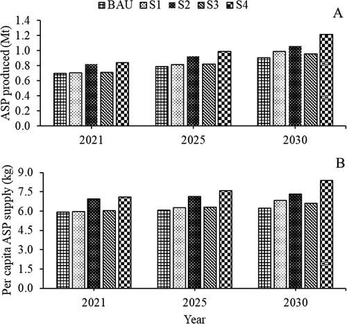
The smallest increases in both ASP produced and supply per capita occurred in the BAU scenario (0.905 Mt and 6.24 kg/person in 2030, respectively), while the highest increase was obtained with S4 (1.214 Mt and 8.38 kg/person in 2030, respectively) (Figure 2). Improving feed digestibility in S2 resulted in higher ASP produced and available per capita than the structural changes in cattle herd and chicken flock composition modelled in S1 and S3 (Figure 2).

Figure 3A and B show that the total GHG emissions from cattle, sheep, goats, and chicken increased as total ASP produced increased, while emission intensities decreased during the period from 2021 to 2030. The highest increase in total GHG emissions by 2030 relative to 2020 was observed in S2 (i.e. increasing from 126.2 MtCO₂e to 152.2 MtCO₂e) while the lowest was observed in S1 (i.e. increasing 124.8 MtCO₂e to 146.7 MtCO₂e). The total increase in GHG emissions from S3 and S4 by 2030 were 18% and 19% respectively relative to 2020.

Figure 3. Impact of simulated intervention strategies on the total greenhouse gas emissions (A) and the emission intensities per unit animal source protein (ASP) in Ethiopia from 2021 to 2030.

BAU: business-as-usual scenario i.e., an extrapolation of the historical trend observed during the base years; S1: improved dairy production scenario by replacing seven million local breeds with 3.6 million cross-breeds; S2: improved dairy production scenario by increasing feed digestibility on mixed crop-livestock farms; S3: improved poultry production scenario via reduced indigenous chicken population, increased hybrid and exotic breeds population, as well as commercial production; and S4: combining all interventions from S1 to S3 within one scenario.

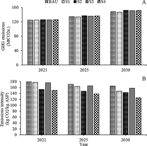
In contrast to total GHG emissions, emission intensities per kg of animal source protein decreased (Figure 3B) across all scenarios until 2030, with the highest and lowest decreases observed in S4 (i.e. 150.7 kg CO₂e to 125.0 kg CO₂e) and the BAU (i.e.,179.2 kg CO₂e to 164.7 kg CO₂e) scenarios, respectively.

Sensitivity analysis

The largest SI and PV for total GHG emissions and ASP output were due to modifications in the livestock population in the mixed crop-livestock and pastoral/agropastoral systems (Table 6). The changes made to the poultry population in different production systems resulted in the lowest SI and PV.

Table 6. Results of sensitivity analysis showing the effect of varying livestock populations on total emissions and total animal source protein outputs in 2020.

Production system/breeds	*Pop2020 (n)	Variation (%)	^#SIemissions (Mt CO2e)	^##PV (%)	^§SIASP (Mt)	^§§PV (%)
Other cattle
Pastoral/agropastoral	12,967,069	+10	0.15	1.5	0.23	2.2
		−10	0.14	-1.5	0.22	-2.2
Mixed crop-livestock	55,496,248	+10	0.68	6.7	0.53	5.2
		−10	0.66	-6.7	0.52	-5.3
Dairy cattle
Smallholder intensive	1,828,458	+10	0.03	0.3	0.13	1.3
		−10	0.03	−0.3	0.12	−1.3
Commercial	668,495	+10	0.01	0.1	0.04	0.4
		−10	0.09	−0.9	0.05	−0.6
Sheep
Pastoral/agropastoral	18,331,072	+10	0.03	0.3	0.01	0.1
		−10	0.03	−0.3	0.01	−0.1
Mixed crop-livestock	24,583,793	+10	0.03	0.3	0.02	0.2
		−10	0.03	−0.3	0.02	−0.2
Goats
Pastoral/agropastoral	30,035,747	+10	0.05	0.4	0.02	0.2
		−10	0.04	−0.4	0.02	−0.2
Mixed crop-livestock	22,427,788	+10	0.03	0.3	0.02	0.2
		−10	0.03	−0.3	0.02	−0.2
Poultry
Indigenous breeds	44,940,924	+10	0.00	0.0	0.00	0.0
		−10	0.00	0.0	0.01	−0.1
Hybrid breeds	5,194,345	+10	0.00	0.0	0.00	0.0
		−10	0.00	0.0	0.00	0.0
Exotic breeds	6,857,718	+10	0.00	0.0	0.00	0.0
	6,857,718	−10	0.00	0.0	0.00	0.0
Commercial breed	4,788,982	+10	0.00	0.0	0.01	−0.1
		−10	0.00	0.0	0.01	−0.1

* Pop₂₀₂₀: The default population of livestock in each production system reported for 2020,

^# SIemissions: the sensitivity index for total greenhouse gases emitted in response to ± 10 % variations in the default livestock population,

^## PV: the percentage variation in total greenhouse gases emissions due to the modified population,

^§ SI_ASP: the sensitivity index for total animal source protein produced due to variations in livestock population, and

^§§ PV: the percentage variation in total animal source protein output due to variations in population.

Of the three emission factors considered in our analysis, modifications to enteric fermentation emission factors resulted in the largest SI and PV (Table 7). In particular, the largest SI and PV were observed when changing the emission factors for cattle in mixed crop-livestock and pastoral/agropastoral systems, while the lowest were observed for sheep and goats. Modifying the emission factors for N₂O yielded the lowest variations in total GHG emissions in cattle, sheep, and goat production systems.

Table 7. Results of sensitivity analysis showing the effect of varying emission factors for different livestock sources on total emissions during a reference year (i.e. 2020).

Production system/breeds	*Emission factors	^&EF2020 (kg/head/yr)	Variation (%)	^#SIemissions (Mt CO2 e)	^##PV (%)
Other cattle
Pastoral/agropastoral	Enteric CH4	46.6	+10	0.14	1.3
			−10	0.13	−1.3
	MMS CH4	2.43	+10	0.01	0.1
			−10	0.01	−0.1
	MMS N2O	0.36	+10	0.01	0.1
			−10	0.01	−0.1
Mixed crop-livestock	Enteric CH4	48.26	+10	0.60	5.9
			−10	0.58	−5.9
	MMS CH4	3.52	+10	0.04	0.4
			−10	0.04	−0.4
	MMS N2O	0.35	+10	0.05	0.5
			−10	0.03	−0.3
Dairy cattle
Smallholder intensive	Enteric CH4	57.55	+10	0.02	0.2
			−10	0.02	-.02
	MMS CH4	15.72	+10	0.01	0.1
			−10	0.01	−0.1
	MMS N2O	0.78	+10	0.00	0.0
			−10	0.00	0.0
Commercial	Enteric CH4	53.17	+10	0.01	0.1
			−10	0.01	−0.1
	MMS CH4	14.15	+10	0.00	0.0
			−10	0.00	0.0
	MMS N2O	0.72	+10	0.00	0.0
			−10	0.00	0.0
Sheep
Pastoral/agropastoral	Enteric CH4	6.59	+10	0.03	0.3
			−10	0.03	−0.3
	MMS CH4	0.14	+10	0.00	0.0
			−10	0.00	0.0
	MMS N2O	0.03	+10	0.00	0.0
			−10	0.00	0.0
Mixed crop-livestock	Enteric CH4	5.72	+10	0.03	0.3
			−10	0.03	−0.3
	MMS CH4	0.13	+10	0.00	0.0
			−10	0.00	0.0
	MMS N2O	0.03	+10	0.00	0.0
			−10	0.00	0.0
Goats
Pastoral/agropastoral	Enteric CH4	6.08	+10	0.04	0.4
			−10	0.04	−0.4
	MMS CH4	0.17	+10	0.00	0.0
			−10	0.00	0.0
	MMS N2O	0.038	+10	0.00	0.0
			−10	0.00	0.0
Mixed crop-livestock	Enteric CH4	5.99	+10	0.03	0.3
			−10	0.03	−0.3
	MMS CH4	0.17	+10	0.00	0.0
			−10	0.00	0.0
	MMS N2O	0.038	+10	0.00	0.0
			−10	0.00	0.0

* Emission factors: MMS CH₄ and MMS N₂O refer to methane emissions and nitrous oxide emissions from the manure management systems respectively,

^& EF₂₀₂₀: The default emission factors estimated using activity data for livestock in each production system reported in the selected year (i.e. 2020),

^# SI_emissions: the sensitivity index for total GHG emissions in response to ± 10 % variations in the default emission factors used during the selected year (i.e. 2020), and

^## PV: the percentage variation in total greenhouse gases emissions due to variations in the emission factor.

Discussion

Historical and projected emissions and emission intensity

The present study showed that during the last decade, total GHG emissions from the main livestock species in Ethiopia increased by 34% in 2020 relative to 2010. This increase was driven by growing livestock populations (especially dual-purpose cattle), with a minor contribution from increased productivity in the smallholder and commercial dairy sectors [31]. Globally, most of the recent and future increase in livestock GHG emissions has been from low- and middle-income countries [8]. The historical trend in total GHG emissions from the major livestock species in Ethiopia has followed the same pattern as in low- and middle-income countries in general (Figure 1). However, the emission intensity per unit ASP produced decreased by 8.8% over the same period in Ethiopia. This is consistent with the long-term trend in low- and middle-income countries, which have contributed most to increased livestock emissions in recent decades, and where emission intensity has decreased at a greater rate than in high income countries [2].

The scenarios (S1 to S4) modelled in the present study showed that the projected total GHG emissions from livestock in Ethiopia will likely continue to increase while emission intensities will decrease. These findings are consistent with the trends in total GHG emissions and emission intensities observed at global level. However, we estimated a slower rate of increase in total GHG emissions in S1 compared to that in the BAU scenario in the present study. Scenario S1 had an average annual increase in total GHG emission of 1.40% between 2021 and 2030 compared to 1.55% in the BAU scenario and resulted in lower total GHG emissions in 2030 (i.e. 146.7 MtCO₂e) than in the BAU scenario (i.e. 149.0 MtCO₂e). The main reason for this was that changes in livestock population structure due to replacing 1.95 indigenous cattle with one crossbred cattle in the mixed crop-livestock system resulted in a lower (i.e. 4% smaller) cattle population in S1 than in the BAU scenario. It is well established that the total GHG emissions from livestock is directly proportional to their population size [27, 45]. It is noteworthy that the per capita supply of ASP by 2030 was higher in S1 (i.e. 6.84 kg/year) than in the BAU scenario (i.e. 6.24 kg/year). This finding stands out because it shows that structural changes in the livestock herd could reduce total GHG emissions and concomitantly increase ASP supply. Thus, in addition to animal- or herd- level technical options frequently investigated in the literature [18, 20,21], sector strategies need to be further investigated to establish their potential to limit and/or reduce livestock GHG emissions in low- and middle-income countries.

For S2, S3 and S4, the projected GHG emissions until 2030 were all higher than in the BAU scenario, implying that no mitigation would be achieved in absolute terms from the implemented strategies. Scenario S3 also involved a structural change strategy in which the indigenous chicken population was reduced while increasing that of hybrid and exotic chickens. A similar reduction in total GHG emissions by 2030 was not observed as in S1 because chickens were responsible for less than 0.2% of all emissions in our study. Considering that it takes about 72 commercial chickens to emit as much as one male cattle in the mixed crop-livestock system (own estimates), a sector strategy focusing only on poultry would need to be at very large scale in order to significantly affect total national livestock GHG emissions. Thus, we deduce that sector transformation strategies could serve as suitable mitigation options if the structural changes in the total population focus on key livestock categories.

National GHG abatement strategies

The livestock sector in most low- and middle-income countries makes significant contributions to food supply, employment and rural incomes [16, 35], as well as to GHG emissions [38, 46]. To reconcile food and income security objectives in the livestock sector with environmental objectives, the right policy options or strategies must be chosen. The policy strategies modelled in the present study were designed to ‘combine mitigation, efficiency gains and output growth in the livestock sector of Ethiopia’ ( [26], page 13). Policy options that promote environmental objectives for the livestock sector include technical options implemented at individual animal or farm level⁵, but also structural options at sub-sector and sector levels [47]. It is not clear whether technical options in general offer a higher potential than structural options to reduce the emission intensity of livestock products [1]. For example, improving feed digestibility (i.e. a technical option) in S2 resulted in a GHG emissions intensity reduction of 20% (i.e. from 179.1 kg CO₂e to 143.4 kg CO₂e) per kg ASP produced between 2020 and 2030 compared to a 17% decrease in S1 when the cattle herd composition was restructured. Yet, both technical and structural change face complex implementation barriers in low- and middle-income countries [22, 46]. For example, feeding oil (lipids) to cattle is another technical option which could help mitigate GHG emissions from cattle in low- and middle-income countries, but it is often not economically feasible. Similarly, structural changes may require that more elements in the enabling environment are put in place, and such systemic changes are more difficult to influence through policy measures. Nevertheless, noting that the mitigation effects (per unit ASP) of S1 and S2 were of the same order of magnitude, we suggest that leveraging structural changes in the livestock sector (as in S1) should be given more attention because these changes may help address food and income security as well as environmental objectives [21] in rapidly growing livestock economies. As discussed in Section 4.1 above, only S1 achieved a reduction in total GHG emissions by 2030 compared to the BAU scenario, which makes it the most potent option for abating GHG emissions in our study. Furthermore, evidence from S4 showed that the greatest benefits in terms of food and income security as well as environmental objectives can be obtained when deploying a package of interventions. Integrated action involving multiple stakeholders is thus crucial to achieve the maximum GHG mitigation potential offered by the livestock sector [48].

Country versus global perspectives

Important differences exist in terms of per capita livestock emissions between low-and middle-income countries and high income countries [8]. For example, global per capita livestock emissions (i.e. direct livestock emissions) in 2020 stood at 0.51 t CO₂e, compared to 1.07 t CO₂e for Ethiopia (low-income country) and 0.77 t CO₂e for the United States (high-income country). On the one hand, these values reflect the higher efficiency of livestock production in high-income countries compared to low-income countries. On the other hand, the per capita emissions show that different solutions would be needed to accommodate the growing livestock sector in low- and middle-income countries. In addition, it is important to note that the focus of the present study was on direct livestock emission sources. However, there are also emissions from other sources in livestock product supply chains in low- and middle-income countries, although they account for a much smaller proportion of total supply chain emissions than in high income countries [27]. This means that in low- and middle-income countries, the current focus for potential GHG mitigation interventions should be on direct livestock emissions, which may be different from the priority for high-income countries.

The academic literature on the contribution of livestock to GHG emissions and the need to reduce consumption of ASP has grown rapidly in recent years and became a choice topic of the media in high-income countries. The EAT Lancet paper [49] in particular has been very influential as it suggested that global climate change boundaries could be kept if the whole global population consumed a relatively low level of ASP per capita. While many such articles and the media may focus on ASP consumption patterns in high income countries, no distinction is often made with respect to low- and middle-income countries. Livestock sector related policies in low- and middle-income countries like Ethiopia must address multiple goals, including nutrition and food security, income growth and employment [16, 50]. The challenge for policy makers in these countries is to balance national development objectives with climate change mitigation objectives. A focus on production efficiency has also been criticized as promoting a narrative of ‘climate change delay’ [24], but it may be an appropriate way to balance multiple objectives in low- and middle-income countries. Many rural people in Ethiopia are mainly (e.g. in Borana) or at least partially dependent on livestock for their livelihoods [51]. On the consumption side, there are both undernourished people (e.g. low ASP consumption among infants and school children) and obesity among some groups, with different challenges among rural and urban groups [37]. Therefore, policy recommendations must always seek to balance livestock production and sustainable national development by providing locally context-specific solutions to the global livestock emission challenges [50].

It is unlikely that a reduction in demand for ASP will occur during the next decade in most low- and middle-income countries. Hence, the need to improve production efficiency while increasing total ASP produced to meet the growing demand [23]. Focusing on improving production efficiency in low- and middle-income countries could accommodate current national development objectives and also pave the way for more ambitious demand-side measures to reduce total GHG emissions under higher productivity in the future [24]. There is a strong correlation between GHG emission intensity per unit ASP and the efficiency of nutrient and digestible energy use in livestock [52,53]. This means that any interventions that improves production efficiency (i.e. emission intensity/kg ASP) could help slow down the rate of growth in total GHG emissions. Evidence from our study shows that the emission intensities per kg ASP were lower in S4, S2, S1 and S3 (from lowest to highest) compared to the BAU scenario in 2030 (Figure 3B). Improving livestock production efficiency may thus by an important way by which low- and middle-income countries can contribute to global climate commitments while addressing national context-specific food and income security issues.

Sensitivity analysis

The results of our analysis suggest that our forecasting approach is suitable to capture the changes in our output parameters of interest (i.e. total GHG emissions and ASP) as a result of variation in the activity data used (i.e. population and emission factors). The total GHG emissions and ASP output in the present study were most sensitive to changes in the size of livestock populations and emission factors in the mixed crop-livestock and pastoral/agropastoral systems. For example, in our scenarios modifying the population of cattle in the mixed crop-livestock system by 10% resulted in 7% and 5% change in the total GHG emissions and ASP output respectively (Table 6). These findings are in line with those reported by [27] and [45], who indicated that livestock population numbers are directly proportional to total GHG emissions. Also, our forecasting approach seems robust because modifying the population size did not result in an equivalent or proportional change in total GHG emissions and ASP output. Although the relationships between these parameters are linear, it is not “one to one” and thus per unit changes in population size resulted in smaller changes in the output variables. Similar to modifications in population size, changes in emission factors also resulted in variations in total GHG emissions, with the largest variations (PV) observed in the mixed crop-livestock and pastoral/agropastoral systems.

The sensitivity analysis also suggests that interventions that target mixed crop-livestock systems and pastoral/agropastoral cattle systems could yield the highest mitigation potential. This is supported by our forecasting analysis in S1 where artificial insemination was used to replace indigenous breeds with cross-bred cattle, which resulted in lower total GHG emissions and more ASP supply per capita than in the BAU scenario. It is important to note that replacing indigenous cattle by cross-bred cattle is not a new practice in Ethiopia but one that has been on-going for years [54]. Such structural changes could be further explored to see how they can contribute to mitigating livestock GHG emissions.

Limitations of this study

The present study has some limitations. First, the projections made for the period between 2021 to 2030 assumed a linear interaction between livestock development strategies, livestock performance, and livestock emissions. However, livestock production systems are complex systems where components interact non-linearly [35]. Whereas our sensitivity analysis suggested that our forecasting approach is robust, the assumptions made in the present study may still lead to under- or overestimations of the modelled outputs. Modelling studies like the present one cannot claim to fully represent reality and often simplify the livestock systems being studied to inform field research [55]. The present study does not claim to have fully captured reality, but we explored different interventions to inform further research on which livestock production strategies have a potential to simultaneously address national development and global climate objectives. Second [31], highlighted and discussed the uncertainty associated with the population and performance activity data for cattle, sheep, and goat production systems modelled in the present study. This uncertainty may also have affected the accuracy of the GHG estimates in the present study.

Conclusions

Our study highlighted how national livestock development strategies can increase ASP production and supply while also reducing total GHG emissions in a low- and middle-income country. The present study revealed that structural changes in the herd composition of key livestock categories (i.e. cattle) resulted in 1.6% less total GHG emissions and 9.6% more ASP supplied per capita in S1 by 2030 compared to the BAU scenario. These findings highlight that, in additional technical options implemented at the individual animal or farm level, more attention should be paid to strategies that promote structural change in the livestock sector. This is because a structural sector transformation could be a highly relevant policy option in the context of rapidly growing livestock sectors in low- and middle-income countries, and may provide ways to simultaneously address multiple goals, including food and income security and global climate commitments. Therefore, there is a need for further studies to assess the true potential of structural strategies in the livestock sector and their impact on total GHG emissions in low- and middle-income countries.

Acknowledgements

The present study was implemented as part of the CGIAR Research Program on Climate Change, Agriculture and Food Security (CCAFS), which was carried out with financial support from the CGIAR Fund Donors and through bilateral funding agreements (see https://ccafs.cgiar.ord/donors).

Disclosure statement

No potential conflict of interest was reported by the author(s).

Data availability statement

All datasets used in the present study are available from the corresponding author upon request.

Notes

1 The summarized data and all details on how the production systems, the animal categories, and productive and reproductive performance were defined and calculated are reported in Annexes 1 to 5 of 55).

2 https://data.un.org/Data.aspx?d=PopDiv&f=variableID%3A12

3 Since the present study was not done using a mean default value at one point in time but over several years, we selected the latest year for which reported data was available (i.e., 2020) as the default mean for our sensitivity analysis.

4 Poultry were not included because the emissions factors used the Tier 1 default values of the IPCC, and thus no changes were made in the present study.

5 This approach is the focus of reviews on livestock mitigation options, e.g. 55), 55), 55).

References

- Gerber JS, Steinfeld H, Henderson B, et al. Tackling climate change through livestock: a global assessment of emissions and mitigation opportunities. Rome: Food and Agriculture Organization of the United Nations; 2013a. 1 online resource (XXI, 115 pagina’s).
- Caro D, Davis SJ, Bastianoni S, et al. Global and regional trends in greenhouse gas emissions from livestock. Climatic Change. 2014;126(1–2):203–216. doi:10.1007/s10584-014-1197-x.
- Lamb WF, Wiedmann T, Pongratz J, et al. A review of trends and drivers of greenhouse gas emissions by sector from 1990 to 2018. Environ Res Lett. 2021;16(7):073005. doi:10.1088/1748-9326/abee4e.
- UNEP/CCAC. (Ed.), Global methane assessment: benefits and costs of mitigating methane emissions. Nairobi, Kenya: United Nations Environment Programme; 2021.
- Turner MC, Jerrett M, Pope CA, et al. Long-term ozone exposure and mortality in a large prospective study. Am J Respir Crit Care Med. 2016;193(10):1134–1142. doi:10.1164/rccm.201508-1633OC.
- Shindell D, Faluvegi G, Kasibhatla P, et al. Spatial patterns of crop yield change by emitted pollutant. Earths Future. 2019;7(2):101–112. doi:10.1029/2018EF001030.
- IPCC. Climate change 2013: the physical science basis: working group I contribution to the Fifth assessment report of the Intergovernmental Panel on Climate Change. Thomas F. Stocker, (Ed.), Working Group I co-chair, University of Bern [and nine others]. New York: Cambridge University Press; 2013.
- FAOSTAT. Emissions totals. Food and Agriculture Organization of the United Nations; 2021. https://www.fao.org/faostat/en/#data/GT. Accessed 18 November 2021.
- Herrero M, Thornton PK. Livestock and global change: emerging issues for sustainable food systems. Proc Natl Acad Sci U S A. 2013;110(52):20878–20881. doi:10.1073/pnas.1321844111.
- Latino LR, Pica-Ciamarra U, Wisser D. Africa: the livestock revolution urbanizes. Glob Food Sec. 2020;26:100399. doi:10.1016/j.gfs.2020.100399.
- UNDESA. World population prospects 2019. United Nations, Department of Economic and Social Affairs, Population Division; 2019. https://population.un.org/wpp/DataQuery/. Accessed 20 December 2019.
- O’Mara FP. The significance of livestock as a contributor to global greenhouse gas emissions today and in the near future. Animal Feed Science and Technology. 2011;166–167:7–15. doi:10.1016/j.anifeedsci.2011.04.074.
- UNFCCC. Adoption of the Paris Agreement. United Nations framework convention on climate change; 2015. https://unfccc.int/resource/docs/2015/cop21/eng/l09r01.pdf. Accessed 1 November 2022.
- Rose S, Khatri-Chhetri A, Stier M, et al. Livestock management ambition in the new and updated nationally determined contributions: 2020-2021: analysis of agricultural Sub-sectors in national climate change strategies. Wageningen, The Netherlands: CGIAR Research Program on Climate Change, Agriculture & Food Security (CCAFS); 2021.
- Rojas-Downing MM, Nejadhashemi AP, Harrigan T, et al. Climate change and livestock: impacts, adaptation, and mitigation. Climate Risk Manage. 2017;16:145–163. doi:10.1016/j.crm.2017.02.001.
- Nouala S, Pica-Ciamarra U, Otte J, et al. Policy Note: investing in livestock to drive economic growth in Africa: rationales and Priorities. ALive Policy Note: Investing in Livestock to Drive Economic Growth in Africa. ALIVE; 2011. http://www.fao.org/ag/againfo/resources/newsletter/docs/policynote-investinginlivestock.pdf. Accessed 8 September 2021.
- Herrero M, Grace D, Njuki J, et al. The roles of livestock in developing countries. Animal. 2013;7 Suppl 1:3–18. doi:10.1017/S1751731112001954.
- Gerber PJ, Hristov AN, Henderson B, et al. Technical options for the mitigation of direct methane and nitrous oxide emissions from livestock: a review. Animal. 2013b;7 Suppl 2:220–234. doi:10.1017/S1751731113000876.
- Gerber PJ, Steinfeld H, Henderson B, et al. Tackling climate change through livestock: a global assessment of emissions and mitigation opportunities/Food and Agriculture Organization of the United Nations. Rome: Food and Agriculture Organization of the United Nations; 2013c.
- Herrero M, Henderson B, Havlík P, et al. Greenhouse gas mitigation potentials in the livestock sector. Nature Clim Change. 2016;6(5):452–461. doi:10.1038/nclimate2925.
- Havlík P, Valin H, Herrero M, et al. Climate change mitigation through livestock system transitions. Proc Natl Acad Sci U S A. 2014;111(10):3709–3714. doi:10.1073/pnas.1308044111.
- Enahoro D, Mason-D’Croz D, Mul M, et al. Supporting sustainable expansion of livestock production in South Asia and Sub-Saharan Africa: scenario analysis of investment options. Global Food Security. 2019;20:114–121. doi:10.1016/j.gfs.2019.01.001.
- Chang J, Peng S, Yin Y, et al. The key role of production efficiency changes in livestock methane emission mitigation. AGU Advances. 2021;2(2):e2021AV000391. doi:10.1029/2021AV000391.
- Rigolot C. Narratives Behind livestock methane mitigation studies matter. AGU Adv. 2021;2(4):e2021AV000526. doi:10.1029/2021AV000526.
- CSA. Agricultural Sample survey 2020/21 [2013 E.C]: report on livestock and livestock characteristics (private peasant holdings) Statistical Bulletin 589. Addis Ababa: Central Statistical Agency of the Federal Democratic Republic of Ethiopia; 2021. https://www.statsethiopia.gov.et/wp-content/uploads/2021/05/REVISED_2013.LIVESTOCK-REPORT.FINAL-1.pdf. Accessed 9 September 2021.
- FDRE. Updated nationally determined contribution. Addis Ababa, Ethiopia: Environment, Forest, and Climate Change Commission of the Federal Democratic Republic of Ethiopia; 2021. https://www4.unfccc.int/sites/ndcstaging/PublishedDocuments/Ethiopia%20First/Ethiopia%27s%20updated%20NDC%20JULY%202021%20Submission_.pdf. Accessed 29 September 2021.
- Opio C, Gerber P, Mottet A, et al. Greenhouse gas emissions from ruminant supply chains – a global life cycle assessment. Rome, Italy: Food and Agriculture Organization; 2013. http://www.fao.org/3/i3461e/i3461e.pdf.
- FAO. Global livestock environmental assessment model: model description Version 2.0. Rome, Italy: Food and Agriculture Organization; 2018. http://www.fao.org/fileadmin/user_upload/gleam/docs/GLEAM_2.0_Model_description.pdf. Accessed 14 September 21.
- FAO, ILRI. Smallholder dairy methodology: draft methodology for quantification of GHG emission reductions from improved management in smallholder dairy production systems using a standardized baseline; 2016. https://cgspace.cgiar.org/handle/10568/77602. Accessed 9 October 21.
- Eshetie T, Hussien K, Teshome T, et al. Meat production, consumption and marketing tradeoffs and potentials in Ethiopia and its effect on GDP growth: a review. J Market Consumer Res. 2018;42:17–24.
- Wilkes A, Wassie SE, Tadesse M, et al. Inventory of greenhouse gas emissions from cattle, sheep and goats in Ethiopia (1994-2018) calculated using the IPCC tier 2 approach. Addis Ababa, Ethiopia: Environment and Climate Change Directorate of the Ministry of Agriculture: CGIAR Research Program on Climate Change, Agriculture and Food Security; 2020. https://ccafs.cgiar.org/resources/publications/inventory-greenhouse-gas-emissions-cattle-sheep-and-goats-ethiopia-1994. Accessed 30 September 2021.
- IPCC. Refinement to the 2006 IPCC guidelines for national greenhouse gas inventories. Kanagawa, Japan: Intergovernmental Panel on Climate Change, IGES; 2019. https://www.ipcc-nggip.iges.or.jp/public/2019rf/index.html. Accessed 10 September 21.
- CSA. Agricultural sample survey 2019/20 [2012 E.C.].: Report on livestcok and livestock characteristics (private peasant holdings) Statistical Bulletin 587. Addis Ababa, Ethiopia: Central Statistical Agency, Federal Democratic Republic of Ethiopia; 2020.
- IPCC. Guidelines for national GHG inventories. Kanagawa, Japan: Intergovernmental Panel on Climate Change, IGES; 2006. https://www.ipcc-nggip.iges.or.jp/public/2006gl/pdf/0_Overview/V0_1_Overview.pdf. Accessed 9 September 21.
- Bateki CA, Cadisch G, Dickhoefer U. Modelling sustainable intensification of grassland-based ruminant production systems: a review. Global Food Security. 2019;23:85–92. doi:10.1016/j.gfs.2019.04.004.
- Bateki CA, van Dijk S, Wilkes A, et al. Meta-analysis of the effects of on-farm management strategies on milk yields of dairy cattle on smallholder farms in the tropics. Animal. 2020;14(12):2619–2627. doi:10.1017/S1751731120001548.
- Blakstad MM, Danaei G, Tadesse AW, et al. Life expectancy and agricultural environmental impacts in Addis Ababa can be improved through optimized plant and animal protein consumption. Nat Food. 2021;2(4):291–298. doi:10.1038/s43016-021-00264-2.
- Bouwman L, Goldewijk KK, van der Hoek KW, et al. Exploring global changes in nitrogen and phosphorus cycles in agriculture induced by livestock production over the 1900-2050 period. Proc Natl Acad Sci U S A. 2013;110(52):20882–20887. doi:10.1073/pnas.1012878108.
- IPCC. Climate Change 2014: contribution of working group III to the Fifth Assessment Report of the Intergovernmental Panel on Climate Change. Geneva, Switzerland: IPCC; 2014. https://ar5-syr.ipcc.ch/ipcc/ipcc/resources/pdf/IPCC_SynthesisReport.pdf. Accessed 21 October 2021.
- Shapiro BI, Gebru G, Desta S, et al. Ethiopia livestock master plan ILRI Project Report. Nairobi, Kenya: International Livestock Research Institute; 2015.
- Tewodros A, Mebrate G. Exotic chicken production performance, status and challenges in Ethiopia. Int J Vet Sci Res. 2019;5(2):039–045. doi:10.17352/ijvsr.000040.
- Félix R, Xanthoulis D. Analyse de sensibilite du modele mathematique" erosion productivity impact calculator"(EPIC) par l‘approche One-Factor-At-A-Time (OAT). Biotechnologie, Agronomie, Société Et Environnement. 2005;9(3):179–190.
- Graux AI, Gaurut M, Agabriel J, et al. Development of the pasture simulation model for assessing livestock production under climate change. Agriculture, Ecosyst Environ. 2011;144(1):69–91. doi:10.1016/j.agee.2011.07.001.
- Laguionie P, Roupsard P, Maro D, et al. Simultaneous quantification of the contributions of dry, washout and rainout deposition to the total deposition of particle-bound 7Be and 210Pb on an urban catchment area on a monthly scale. J Aerosol Sci. 2014;77:67–84. doi:10.1016/j.jaerosci.2014.07.008.
- Tongwane MI, Moeletsi ME. A review of greenhouse gas emissions from the agriculture sector in africa. Agricultural Syst. 2018;166:124–134. doi:10.1016/j.agsy.2018.08.011.
- Herrero M, Thornton PK, Gerber P, et al. Livestock, livelihoods and the environment: understanding the trade-offs. Curr Opin Environ Sustainability. 2009;1(2):111–120. doi:10.1016/j.cosust.2009.10.003.
- Frank S, Beach R, Havlík P, et al. Structural change as a key component for agricultural non-CO2 mitigation efforts. Nat Commun. 2018;9(1):1060. doi:10.1038/s41467-018-03489-1.
- Harrison MT, Cullen BR, Mayberry DE, et al. Carbon myopia: the urgent need for integrated social, economic and environmental action in the livestock sector. Glob Chang Biol. 2021;27(22):5726–5761. doi:10.1111/gcb.15816.
- Willett W, Rockström J, Loken B, et al. Food in the anthropocene: the EAT–lancet commission on healthy diets from sustainable food systems. The Lancet. 2019;393(10170):447–492. doi:10.1016/S0140-6736(18)31788-4.
- Mehrabi Z, Gill M, van Wijk M, et al. Livestock policy for sustainable development. Nat Food. 2020;1(3):160–165. doi:10.1038/s43016-020-0042-9.
- Megersa B, Markemann A, Angassa A, et al. The role of livestock diversification in ensuring household food security under a changing climate in Borana, Ethiopia. Food Sec. 2014;6(1):15–28. doi:10.1007/s12571-013-0314-4.
- Yan T, Mayne CS, Gordon FG, et al. Mitigation of enteric methane emissions through improving efficiency of energy utilization and productivity in lactating dairy cows. J Dairy Sci. 2010;93(6):2630–2638. doi:10.3168/jds.2009-2929.
- White RR. Increasing energy and protein use efficiency improves opportunities to decrease land use, water use, and greenhouse gas emissions from dairy production. Agricultural Syst. 2016;146:20–29. doi:10.1016/j.agsy.2016.03.013.
- Feyissa AA, Senbeta F, Tolera A, et al. Unlocking the potential of smallholder dairy farm: evidence from the Central highland of Ethiopia. J Agriculture Food Res. 2022;11:100467.
- Reilly M, Willenbockel D. Managing uncertainty: a review of food system scenario analysis and modelling. Philos Trans R Soc Lond B Biol Sci. 2010;365(1554):3049–3063. doi:10.1098/rstb.2010.0141.