Comparing greenhouse gas footprints and payback times of crop-based biofuel production worldwide

Abstract

Two metrics are typically used to quantify the full greenhouse gas (GHG) balance of biofuel production: the GHG footprint (in kg CO₂-eq/MJ bioenergy produced) and the GHG payback time (in years). The goal of the present study was to quantify and compare spatially explicit GHG footprints and payback times of crop-based bioethanol and biodiesel production, focusing on locations where the four main feedstocks – corn, sugarcane, soybean and rapeseed – are currently cultivated. The largest GHG footprints and longest payback times were found for sugarcane in the tropics, owing to large original carbon stocks in the tropical ecoregions. The lowest GHG footprints and shortest payback times were found in the temperate ecoregions of the USA and Europe, with relatively low initial carbon stocks. For corn, GHG footprints were below the fossil reference and payback times were shorter than 30 years in 71–74% of cumulative production (for sugarcane, in 29–30% of the cumulative production). Soybean and rapeseed have intermediate results, at 49–62% of the cumulative production. The two metrics were highly correlated, except for locations where an infinite payback time was calculated. Overall, GHG footprints and payback times yield similar results when it comes to quantifying GHG balances of biofuels.

Keywords:

• First-generation biofuels
• GHG footprints
• GHG payback times
• land transformation
• land occupation
• metrics

Introduction

Numerous national and international biofuel policies have led to biofuels becoming a considerable energy source for road transportation over the last decades [1, 2]. For example, the USA created the Renewable Fuel Standard Program to raise the share of renewable fuels to almost 10% between 2005 and 2017 [3]. Likewise, the Directive on the Promotion of Use of Biofuels encourages EU Member States to achieve at least a 10% share of biofuels in total transport-related fuel consumption by 2020 [4]. Investing in biofuels is considered to be an important strategy to reach the 2016 Paris Agreement goals [5]. One reason for governments to promote use of biofuels is that they were commonly considered to be a cleaner alternative to fossil fuels when it comes to greenhouse gas (GHG) emissions [6, 7]. However, biofuel production may be associated with land-use change and related biogenic carbon emissions, as it requires fertile agricultural land for feedstock cultivation [8]. Given that croplands generally store less carbon and nitrogen in their soil and biomass than the original natural vegetation, land transformation often causes a net loss of GHGs to the atmosphere that may be attributed to the biofuel production in that location [9, 10]. Studies that account for GHG emissions related to transformation of natural vegetation into croplands find that these emissions can be significant contributors to the GHG balance of biofuels, and thereby determine to what extent biofuels are advantageous over fossil fuels from a GHG perspective [11–15].

Two metrics, typically used to quantify the full GHG balance of biofuel production, are the GHG footprint (in kg CO₂-eq/MJ bioenergy produced) and the GHG payback time (in years) [16]. An advantage of the footprint approach is that it allows for easy comparison with a wide variety of other energy sources, as shown for example by Hoefnagels et al. [17] and Kendall and Yuan [18]. GHG footprints have been derived for a wide variety of first-generation biofuel production systems [e.g. 17, 19–21]. For the GHG payback times metric (GPBTs), the initial GHG emissions from land transformation are considered an ‘investment’ that can be ‘paid back’ if the fossil fuel is replaced by a biofuel with lower fossil GHG emissions during production and use for a certain period [11, 12, 15, 22]. Therefore, the GPBT provides insight into how long biofuels should be produced on the same location before they can be considered a preferable alternative to their fossil counterparts. GPBTs for crop-based biofuels have been derived at the country and continental scale [12, 13, 23], and at the global scale [15, 24]. GHG footprints and GPBTs require mostly the same data inputs, but calculations are done in a different way. To our knowledge, it has not been investigated whether the two metrics yield the same conclusions when quantifying the total GHG balance of biofuels.

Here, we quantified and compared spatially explicit GHG footprints and GPBTs for a selection of crop-based biofuels on a 5-minute grid resolution worldwide. We focused on production of corn- and sugarcane-based bioethanol, and rapeseed- and soybean-based biodiesel, which represent almost 90% of the global biofuel production [25].

Materials and methods

Framework

GHG footprints

GHG footprints were calculated using Equation (1)(1) $${\mathit{GHG}}_{\mathit{biofuel},x,i,j}=\frac{\frac{{\mathit{GHG}}_{\mathit{biogenic},i}}{\mathit{LT}}+{\mathit{GHG}}_{\mathit{prod},x,i,j}}{Y_{x,i,j}\times {\mathit{BF}}_x\times E_x}$$(1) : (1) $${\mathit{GHG}}_{\mathit{biofuel},x,i,j}=\frac{\frac{{\mathit{GHG}}_{\mathit{biogenic},i}}{\mathit{LT}}+{\mathit{GHG}}_{\mathit{prod},x,i,j}}{Y_{x,i,j}\times {\mathit{BF}}_x\times E_x}$$(1) where

GHG_{biofuel,x,i,j} = the GHG footprint of biofuel production for each combination of crop x at location i for management strategy j (in kg CO₂-eq/MJ of bioenergy produced);

GHG_biogenic,i = the biogenic GHG emission from natural biomass and soil upon land transformation for location i (in kg CO₂-eq/ha);

LT = the time the agricultural field is in production (set at a default period of 30 years);

GHG_prod,x,i,j = the GHG emission during production and use of chemicals and farm machinery, including fertilizer application, of crop x at location i for management strategy j (in kg CO₂-eq/ha/year);

Y_x,i,j = the yield of crop x at location i for management strategy j (in kg crop/ha/year);

BF_x = the biofuel conversion efficiency of crop x (in kg biofuel/kg crop); and

E_x = the energy content of a biofuel derived from crop x (in MJ/kg biofuel).

Three farm management strategies with different nitrogen and irrigation inputs were accounted for: (1) no-input, rain-fed; (2) high-input, rain-fed; and (3) high-input, irrigated farming. If a location contains multiple farm management strategies for cultivation of a particular crop, GHG footprints are calculated for each farm strategy, and outcomes were considered separately for all analyses. Only for the creation of geographic information system (GIS) maps, a weighted average was calculated based on the share of these management strategies in the total production of the grid cell.

GHG payback times

GPBTs were calculated for combinations of crop type x, location i, and management strategy j, using Equation (2)(2) $${\mathit{GPBT}}_{\mathit{biofuel},x,i,j}=\frac{{\mathit{GHG}}_{\mathit{biogenic},i}}{{\mathit{GHG}}_{\mathit{bm},x}\times \mathrm{ }{Y_{x,i,j}\times {\mathit{BF}}_x\times E_x-\mathit{GHG}}_{\mathit{prod},x.i.j}}$$(2) : (2) $${\mathit{GPBT}}_{\mathit{biofuel},x,i,j}=\frac{{\mathit{GHG}}_{\mathit{biogenic},i}}{{\mathit{GHG}}_{\mathit{bm},x}\times \mathrm{ }{Y_{x,i,j}\times {\mathit{BF}}_x\times E_x-\mathit{GHG}}_{\mathit{prod},x.i.j}}$$(2) where

GPBT_{biofuel,x,i,j} = the GHG payback time (in years); and

GHG_bm,x = the GHG emission of fossil fuel production that is replaced by biofuel from crop x (in kg CO₂-eq/MJ of fossil energy produced).

This equation may yield negative outcomes when the cropland has a larger total biogenic carbon stock than the original vegetation (i.e. negative GHG_biogenic), or when the ongoing GHG emissions during biofuel production exceed the GHG emissions of fossil fuel production. The first situation translates to an instant payback of the GHG emissions from land transformation (i.e. 0 years), while the latter means that no payback will ever be achieved (i.e. infinite years) [15].

Data input

Yields, conversion efficiencies and energy densities

Locations of feedstock cultivation, yields and cropland area under different farm management strategies were collected from the 2005 Spatial Production Allocation Model (SPAM), which estimates crop distribution, yields and area at a 5-minute resolution based on production statistics, land cover, and the suitability of landscape, climate and soil [26]. We included all locations of corn, sugarcane, rapeseed, and soybean production, assuming that all production locations could potentially contribute to biofuel production. The conversion efficiencies of the different feedstocks and energy densities of the different biofuels are provided in Table S1.

Biogenic GHG emissions

In each location where one of the four biofuel feedstocks is cultivated (based on SPAM), we calculated the biogenic GHG emissions, i.e. emissions of carbon dioxide (CO₂) and nitrous oxide (N₂O) from the soil and biomass due to land transformation and occupation. These biogenic GHG emissions were derived using Equation (5)(5) $${\mathit{GHG}}_{\mathit{biogenic}}=\left(\Delta {\mathit{GHG}}_{\mathit{soil}}\mathrm{ }+\mathrm{ }{\Delta \mathit{GHG}}_{\mathit{biomass}}\right)$$(5) : (5) $${\mathit{GHG}}_{\mathit{biogenic}}=\left(\Delta {\mathit{GHG}}_{\mathit{soil}}\mathrm{ }+\mathrm{ }{\Delta \mathit{GHG}}_{\mathit{biomass}}\right)$$(5) where

ΔGHG_soil = the difference in soil carbon and nitrogen stocks between the natural ecosystem and the cropland in a certain grid cell, expressed in kg CO₂-eq/ha;

ΔGHG_biomass = the difference in biomass carbon stocks between the natural ecosystem and the cropland in a certain grid cell, expressed in kg CO₂-eq/ha.

We used the ecoregion map from Olsen et al. [27] to determine whether the reference vegetation of a certain location was forest or grassland. Carbon stocks of natural forest biomass and soil organic carbon (SOC) contents of natural forests and croplands were collected from the Global Trade and Analysis Project [28]. The carbon stocks of natural grassland biomass were collected from Ruesch and Gibbs [29]. The SOC of natural grasslands was derived for 18 agro-ecological zones (AEZs) around the globe, using the Harmonized World Soil Database (FAO et al. 2012) [30](see Supporting Information S1 for more details). For the changes in SOC stocks upon land transformation, we focused on the top 30 cm of soil. Emissions of N₂O resulting from soil mineralization were assumed to be directly proportional to the loss of soil carbon, following Flynn et al. [31]. Finally, the carbon stored in crop biomass was set to zero because annual harvesting of crops hinders the long-term storage of carbon [15].

GHG emissions related to biofuel and fossil fuel production

Emissions of fossil CO₂, fossil methane (CH₄) and N₂O related to biofuel production were collected from the ecoinvent v. 3 Life Cycle Inventory database [32]. This includes emissions due to energy and material use during agricultural processes such as sowing, plowing, harvesting, and the production and application of pesticides, phosphorus fertilizers, and irrigation water, as well as during the refining process (i.e. esterification of oils and fermentation of sugars). These emission data are feedstock specific, but generic for different countries. Only N₂O emissions related to nitrogen fertilizer application were derived in a spatially explicit manner. Application rates of nitrogen fertilizer under high-input, rain-fed and high-input, irrigated management were calculated with the Environmental Policy Integrated Climate (EPIC) crop growth simulation model [33]. Corresponding N₂O emissions were calculated as per Shcherbak et al. [34]. More details on the calculation of GHG emissions related to nitrogen fertilizer application can be found in the Supplementary material.

GHG emissions during the production and combustion of unleaded petrol and fossil diesel, required for the GPBT calculations, were also collected from ecoinvent [32]. Unleaded petrol and fossil diesel would be replaced by bioethanol and biodiesel, respectively. Fossil benchmarks of 8.8 × 10⁻² and 8.2 × 10⁻² CO₂-eq/MJ were calculated for petrol and diesel, respectively. The same fuel production process (and corresponding GHG emission) was assumed for all countries.

Allocation

We allocated the GHG emissions related to biofuel production between the main product (i.e. bioethanol or biodiesel) and any major by-products of crop cultivation (e.g. corn stover, rapeseed straw) and crop refining (e.g. distillers grains from corn, meal and glycerine from soybean) based on their respective economic values. Economic allocation is recommended for production systems where main products and by-products have different end uses [35] (Wang et al. 2011)[36], and has been adopted by earlier studies on biofuel-related payback times as well [11]. The allocation factors can be found in the Supplementary material (Table S2).

Results

GHG footprints and GPBTs were calculated for a total of 225,715 combinations of crop type, management type and location, located throughout 27,821 different grid cells around the globe, 152 countries and all continents except Antarctica. The results for the footprints and GPBTs and a comparison thereof are presented below.

GHG footprints

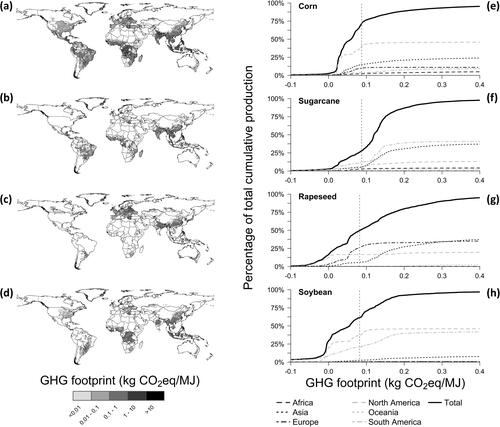
The production-weighted average GHG footprint of biofuels was 0.11 kg CO₂-eq/MJ of bioenergy. The production-weighted average footprints of corn, sugarcane, rapeseed and soybean were 0.11, 0.13, 0.12 and 0.08 kg CO₂-eq/MJ, respectively. The largest footprints were found in the tropical regions, where croplands replaced carbon-rich rainforests (Figure 1a–d). Footprints smaller than the fossil reference were particularly found in temperate regions, including the cases of corn and soybean production in the USA and rapeseed production in most of Europe. The cumulative biofuel production in relation to the GHG footprint shows that 29–71% of the cumulative potential biofuel production stays below the fossil reference, with sugarcane at the low end and corn at the high end of the range (Figure 1e–h).

Figure 1. Spatial distribution of grid-specific greenhouse gas (GHG) footprints around the world (a–d) and relative cumulative production of bioenergy from bioethanol and biodiesel in relation to these GHG footprints (e–h). Dotted lines represent the GHG footprint of the fossil benchmarks, i.e. 8.8 × 10⁻² and 8.2 × 10⁻² kg CO₂-eq per MJ for petrol and diesel, respectively.

GHG payback times

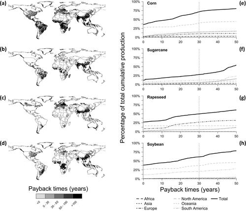
Similar to the GHG footprints, the longest GPBTs were found in the tropical regions (Figure 2a–d). GPBTs of 0 years were found in almost 11% of the calculations, resulting from cropland carbon stocks that exceed the natural reference carbon stocks. This was especially notable in the central USA, where we found that the SOC of croplands often exceeded the summed SOC and biomass carbon of the original mixed and short grassland vegetation. Infinite GPBTs were found in 6% of the calculations, indicating that the initial GHG emissions from land transformation could never be paid back, because the GHG emissions due to yearly biofuel production exceed those of fossil fuel production. When comparing different management strategies in the same location, corn was found to have the longest GPBTs when cultivated under high-input, irrigated farm management, while the GPBTs for soybean were longest under no/low-input, rain-fed management. The cumulative biofuel production in relation to the GPBT shows that 30–74% of the cumulative potential biofuel production stays below the 30 years, with corn at the high end and sugarcane at the low end of the range (Figure 1e–h).

Figure 2. Spatial distribution of grid-specific greenhouse gas payback times (GPBTs) around the world (a–d) and relative cumulative production of bioenergy from bioethanol and biodiesel in relation to these GPBTs (e–h). Dotted lines represent a GPBT of 30 years. For the creation of maps, when data were available for multiple management strategies within one grid cell, a weighted average was calculated based on the share of these management strategies in the total production of this grid cell, but excluding infinite values.

Comparison between footprints and payback times

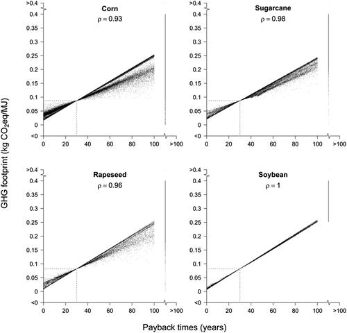
As both GHG footprints and payback times were derived at a grid-specific level, we can assess whether the two metrics lead to the same conclusions. The Spearman rank correlation coefficients are between 0.93 and 1.00 for the four crops considered, indicating very high to near complete overlap in ranks among indicators (Figure 3). In other words, locations found to be favorable according to the GHG footprint are often also favorable according to the GBPT and vice versa. An exception to this trend is found for a number of locations where the payback time is infinite but the corresponding GHG footprint is still smaller than the fossil reference. This combination is found for 0.7, 0.2 and 0.4% of the grid cells for corn, sugarcane and rapeseed, respectively, and for none of the soybean grid cells. This is the result of a combination of GHG emissions during biofuel production that exceed the GHG emissions of fossil fuel production, in locations with high crop yields.

Figure 3. Comparison of greenhouse gas (GHG) footprints and GHG payback times (GPBTs) for four biofuel feedstocks. Each data point is a combination of crop, management strategy, and grid cell. The ρ is the Spearman rank correlation coefficient between the GHG footprints and GHG payback times for each crop.

Discussion

Interpretation

Our study shows that it is possible to reduce GHG emissions by replacing fossil fuels with biofuels, but only when the locations for feedstock cultivation are carefully chosen. We found that corn has the most potential, as its GHG footprints are, on average, the smallest and its payback times are the shortest, while sugarcane has the highest GHG footprints and payback times. In contrast to our findings, previous work showed that the growth characteristics and crop-to-fuel ratios of sugarcane are in fact advantageous compared to other feedstocks [e.g. 11, 12], so our results must be explained by its cultivation solely in tropical and subtropical regions with large natural biogenic carbon stocks that are released after land transformation. This also implies that, despite the better overall outcomes for soybean in the present study, it would hardly be a better alternative to sugarcane when grown in these same tropical regions. Corn, rapeseed and soybean all perform better when grown in the temperate regions, as biogenic carbon emissions are lower there. This may suggest that biofuel production should be located in these temperate regions, but it would only improve the global GHG balance if indirect land use change (ILUC) in the tropics can be mitigated [37].

The comparison of the GHG footprints and payback times showed that there is a high correlation between the two metrics (rho = 0.93–1.00). This finding implies that the two metrics typically provide the same insights in the comparison between crops and between sites. The most important difference between these metrics is the fact that calculation of the GHG footprint requires making an assumption about the number of years the agricultural field will be in production, i.e. the lifetime LT, as the biogenic emissions from land transformation must be allocated over all crops produced during this period. Some small-scale case studies may have real data or realistic estimates of these lifetimes. However, global studies like the present one cannot identify these lifetimes in a spatially explicit manner and are therefore likely to use a generic number, which introduces uncertainty in the outcomes. This uncertainty can be avoided by calculating GPBTs, which use time as an outcome rather than an input. However, if the yield-corrected fossil benchmark provides a slightly lower GHG emission compared to GHG emissions of the biofuel production (in kg CO₂/ha/year), the payback time becomes infinite without further specification in the range. In contrast, the footprint metric provides a more continuous and natural range over the sites and crops. Furthermore, footprints are more straightforwardly compared with the GHG life-cycle emissions of the fossil reference, or other energy sources [e.g. 17].

Uncertainties and assumptions

The outcomes of our study should be interpreted in consideration of several assumptions and uncertainties regarding the methodology and data selection. For instance, we did not account for ILUC that may occur when current cropland is now used to cultivate biofuel crops and food/feed is sourced from elsewhere. ILUC is considered to be an important driver of deforestation worldwide [38, 39]. It could be argued that the reference state of the location where food or feed production is displaced to in favor of biofuel production should be used in our calculations. Following this line of reasoning, producing biofuels in a location with a short payback time or small footprint could induce crop production for food or feed purposes elsewhere, where payback times and footprints are less optimal. Previous work concludes that the use of (soy) biodiesel results in more ILUC than the use of (corn) bioethanol, in part due to its low yield and demand as vegetable oil [40]. However, the impact of ILUC varies with the location of crop production, which in turn depends on complex economic and political considerations. Covering these complex dynamics was beyond the scope of the current work.

Second, we assumed a default plantation time of 30 years for the GHG footprint calculations without considering the exact point in time that cropland was established. For croplands established more than 30 years ago, it may, however, be argued that the initial biogenic carbon emissions should not be included in the GHG footprint calculations of current crop production [see e.g. 41]. Well-established empirical plantation times of croplands would certainly help to improve the GHG footprint calculations in this respect.

It should further be noted that the calculations of the GHG footprints and GPBTs are influenced by the allocation method adopted. Here we allocated the GHG emissions between the biofuel and any by-products based on their respective economic values. Of the three main allocation methods proposed by the International Organization for Standardization ISO 14040, the economic method allocates the largest percentage of emissions to the biofuel. In other words, the footprints and GPBTs would have turned out smaller if energy-based allocation was adopted.

Negative GPBTs were found in the present study, which means that in certain locations cropland soils contain more carbon and nitrogen than did the original ecosystem’s soil and biomass. This is especially notable in the steppes and prairies of the central US and southern Canada, due to relatively low estimates of SOC in natural grasslands and relatively large estimates of SOC in croplands. However there is too little previous work available to validate our input data in this region. One exception is the work by Burke et al. [42], who report SOC stocks in natural grasslands of the central US to be approximately 30–50 Mg C/ha, where we found an average SOC of 37.7 Mg C/ha. Regarding the croplands, Gibbs et al. [28] state that the SOC stocks they provide are likely overestimations, but they do not quantify the expected difference.

Conclusions

Our study shows that corn has the lowest GHG footprints and payback times of the four crops considered. In contrast, sugarcane showed relatively high GHG footprints and payback times due to relatively large biogenic emissions following the clearing of natural vegetation in tropical regions. Corn has GHG footprints below the fossil reference and GPBTs shorter than 30 years in 71–74% of cumulative production, while for sugarcane this is this case in 29–30% of the cumulative production. For soybean and rapeseed, 49–62% of the cumulative production has a GHG footprint lower than the fossil reference and GPBTs shorter than 30 years. The two metrics were highly correlated, implying that the selection of either one of these metrics is typically a matter of taste.

Acknowledgements

The authors wish to thank Erwin Schmid (BOKU) for running the EPIC model simulations. PE was financed by FP7-grant DESIRE (ENV.2012.6.3-3) and MH was financed by the ERC-Consolidation Grant SIZE (Proposal No. 647224).

Disclosure statement

No potential conflict of interest was reported by the authors.

Additional information

Funding

The authors wish to thank Erwin Schmid (BOKU) for running the EPIC model simulations. PE was financed by FP7-grant DESIRE (ENV.2012.6.3-3) and MH was financed by the ERC-Consolidation Grant SIZE (Proposal No. 647224).

References

- Goldemberg J, Mello FFC, Cerri CEP, et al. Meeting the global demand for biofuels in 2021 through sustainable land use change policy. Energy Policy. 2014;69:14–18.
- Su Y, Zhang P, Su Y. An overview of biofuels policies and industrialization in the major biofuel producing countries. Renew Sustain Energy Rev. 2015;50:991–1003.
- US EPA. (2005). Renewable Fuel Standard Program. Available from https://www.epa.gov/renewable-fuel-standard-program.
- Renewable Energy Directive. 2009. Available from http://ec.europa.eu/energy/en/topics/renewable-energy/biofuels.
- Goldemberg J. How much could biomass contribute to reaching the Paris Agreement goals? Biofuels Bioprod Bioref. 2017;11:237–238.
- Goldemberg J, Coelho ST, Lucon O. How adequate policies can push renewables. Energy Policy. 2004;32:1141–1146.
- Thompson W, Whistance J, Meyer S. Effects of US biofuel policies on US and world petroleum product markets with consequences for greenhouse gas emissions. Energy Policy. 2011;39:5509–5518.
- Daioglou V, Doelman JC, Stehfest E, et al. Greenhouse gas emission curves for advanced biofuel supply chains. Nature Clim Change. 2017;7:920–924.
- Danielsen F, Beukema H, Burgess ND, et al. Biofuel plantation on forested lands: Double jeopardy for biodiversity and climate. Conserv Biol. 2009;23:348–358.
- Müller-Wenk R, Brandão M. Climatic impact of land use in LCA – carbon transfers between vegetation/soil and air. Int J Life Cycle Assess. 2010;15:172–182.
- Fargione J, Hill J, Tilman D, et al. Land clearing and the biofuel carbon debt. Science 2008;319:1235–1238.
- Gibbs HK, Johnston M, Foley JA, et al. Carbon payback times for crop-based biofuel expansion in the tropics: The effects of changing yield and technology. Environ Res Lett. 2008;3:1–10.
- Searchinger T, Heimlich R, Houghton RA, et al. Use of U.S. croplands for biofuels increases greenhouse gases through emissions from land-use change. Science 2008;319:1238–1240.
- Hallgren W, Schlosser CA, Monier E, et al. Climate impacts of a large-scale biofuels expansion. Geophys Res Lett. 2013;40:1624–1630.
- Elshout PMF, Van Zelm R, Balkovic J, et al. Greenhouse-gas payback times for crop-based biofuels. Nature Clim Change. 2015;5:604–610.
- Malça J, Freire F. Life-cycle studies of biodiesel in Europe: a review addressing the variability of results and modeling issues. Renew Sustain Energy Rev. 2011;15:338–351.
- Hoefnagels R, Smeets E, Faaij A. Greenhouse gas footprints of different biofuel production systems. Renew Sustain Energy Rev. 2010;14:1661–1694.
- Kendall A, Yuan J. Comparing life cycle assessments of different biofuel options. Curr Opin Chem Biol. 2013;17:439–443.
- Hammond GP, Seth SM. Carbon and environmental footprinting of global biofuel production. Appl Energy. 2013;112:547–559.
- Pfister S, Scherer L. Uncertainty analysis of the environmental sustainability of biofuels. Energy, Sustain Soc. 2015;5:30.
- Mekonnen MM, Romanelli TL, Ray C, et al. Water, energy, and carbon footprints of bioethanol from the U.S. and Brazil. Environ Sci Technol. 2018;52:14508–14518.
- Nguyen TH, Williams S, Paustian K. Impact of ecosystem carbon stock change on greenhouse gas emissions and carbon payback periods of cassava-based ethanol in Vietnam. Biomass Bioenergy. 2017;100:126–137.
- Kim H, Kim S, Dale BE. Biofuels, land use change, and greenhouse gas emissions: Some unexplored variables. Environ Sci Technol. 2009;43:961–967.
- Yang Y, Suh S. Marginal yield, technological advances, and emissions timing in corn ethanol’s carbon payback time. Int J Life Cycle Assess. 2015;20:226–232.
- Searchinger T, C, Hanson, J, Ranganathan et al. Creating a Sustainable Food Future: A Menu of Solutions to Sustainably Feed More Than 9 Billion People by 2050. Washington D.C., World Resources Institute, World Bank, UNEP and UNDP. World Resources Report 2013-14: Interim Findings, 2013.
- You L, U, Wood-Sichra, S, Fritz et al. (2014). Spatial Production Allocation Model (SPAM) 2005 v2.0. May 22, 2015. Available from http://mapspam.info.
- Olsen DM, Dinerstein E, Wikramanayake ED, et al. Terrestrial ecoregions of the world: A new map of life on earth. BioScience 2001;51:933–938.2.0.CO;2]
- Gibbs HK, Yui S, Plevin RJ. New estimates of soil and biomass carbon stocks for global economic models. GTAP Technical Paper No.33, 2014.
- Ruesch A, Gibbs HK. (2008). New IPCC Tier-1 Global Biomass Map for the Year 2000. Oak Ridge National Laboratory, Oak Ridge, Tennessee, Available online from the Carbon Dioxide Information Analysis Center. Available from http://cdiac.ornl.gov.
- FAO, IIASA, ISRIC, ISSCAS and JRC (2012). Harmonized World Soil Database (version1.2) Rome Italy and IIASA Laxenburg, Austria.
- Flynn HC, Canals L. M I, Keller E, et al. Quantifying global greenhouse gas emissions from land-use change for crop production. Glob Change Biol. 2012;18:1622–1635.
- Weidema BP, C, Bauer, R, Hischier, et al. Overview and methodology. Data Quality Guideline for the ecoinvent database version 3. St. Gallen, The Ecoinvent Centre. Ecoinvent Report. 2013;1.
- Williams JR, Jones CA, Dyke PT. A modeling approach to determining the relationship between erosion and soil productivity. Trans ASAE. 1984;27:129–0144.
- Shcherbak I, Millar N, Robertson GP. Global metaanalysis of the nonlinear response of soil nitrous oxide (N2O) emissions to fertilizer nitrogen. Proc Natl Acad Sci USA. 2014;111:9199–9204.
- ISO. (1997). Environmental management – Life cycle assessment – Principles and framework, ISO 14040, 1st ed., June.
- Wang, M, Huo, H, Arora, S. Methods of dealing with co-products of biofuels in life-cycle analysis and consequent results within the U.S. context. Energy Policy. 2011;39:5726–5736. doi:https://doi.org/10.1016/j.enpol.2010.03.052.
- Gerssen-Gondelach SJ, Wicke B, Faaij APC. GHG emissions and other environmental impacts of indirect land use change mitigation. GCB Bioenergy. 2017;9:725–742.
- Lambin EF, Meyfroidt P. Global land use change, economic globalization, and the looming land scarcity. Proc Natl Acad Sci USA. 2011;108:3465–3472.
- Matthew K, Griffin WM, Matthews HS. Indirect land use change and biofuel policy. Environ Res Lett. 2009;4:034008.
- Broch A, Hoekman SK, Unnasch S. A review of variability in indirect land use change assessment and modeling in biofuel policy. Environ Sci Policy. 2013;29:147–157.
- Garcia R, Freire F. Carbon footprint of particleboard: a comparison between ISO/TS 14067, GHG Protocol, PAS 2050 and Climate Declaration. J Clean Prod. 2014;66:199–209.
- Burke IC, Yonker CM, Parton WJ, et al. Texture, climate and cultivation effects on soil organic matter content in U.S. grassland soils. Soil Sci Soc Am J. 1989;53:800–805.