Detection and characterisation of short fatigue cracks by inductive thermography

ABSTRACT

Inductive thermography can be excellently used to detect surface cracks in metals. A short induction heating pulse (0.1-1s) induces eddy currents in the sample and an infrared camera records the surface temperature distribution. As cracks disturb the eddy current distribution and the heat diffusion, they become visible in the infrared images. In this paper it is investigated, how different parameters influence the surface pattern around short cracks (0.5-12mm length). The main emphasis is on finite element simulations, but some experimental results are presented, too. The influence of crack geometry, as crack depth, length, inclination angle and crack shape below the surface are investigated for ferro-magnetic and austenitic steel. Around the crack tips high temperature ‘hot spots’ can be observed, which intensity increases with the crack depth. But this intensity is strongly affected by the crack shape, whether it is rectangular, trapezoid or half-penny shape. For longer cracks (6-8mm length) simulation results show, that in the middle of the crack the phase distribution can be used to estimate the crack depth. Furthermore, the effect of experimental parameters, as excitation frequency, heating pulse duration and the angle between crack line and induction coil are investigated in order to optimize an experimental setup.

KEYWORDS:

• Thermography
• induction thermography
• crack detection
• crack depth
• crack length
• crack shape

Introduction

In the case of inductive thermography the work-piece is heated with a short (0.1–1 s) inductive heating pulse and an infrared (IR) camera records the surface temperature. A surface breaking crack disturbs the eddy current distribution as the current flows around it, causing a local inhomogeneous heating around the crack. Additionally, the heat flux is also affected by the crack. Due to these two effects surface cracks can be excellently detected in metallic surfaces by evaluating the infrared images. The technique is non-destructive and contact-free and it can be fully automated using image processing methods.

In the last few years, several investigations have been published proving the applicability of this method. The first industrial application was reported around 30 years ago [1]. Steel bars and billets were tested for surface cracks during motion through an induction coil and by evaluating the signal of four infrared line scanners placed around the steel bar. In the last 20 years, FPA (focal-plane-array) cameras became more powerful and dropped in price, initiating more scientific research in the area of thermographic inspection [2]. Inductive thermography is one of the active thermography methods, which have been studied and developed by several groups in the few last years. The working group around Busse investigated induction thermography to detect subsurface defects in steel and in CFRP (carbon fibre reinforced polymer) samples in a modulated way (lock-in technique) and with pulse heating (burst thermography) [3]. Aluminium fatigue surface cracks have been also detected using the lock-in technique [4]. Analytical and numerical models [5–7] have been set up for modelling cracks perpendicular to the surface in steel materials. In these simplified models, the cracks were modelled either as a long notch or as a short slot going through the whole sample thickness [6,7]. Experimental results for surface crack detection with induction thermography have been reported by several groups in different ferro-magnetic samples, for example, in forged parts [8,9] and in rail surfaces [10–12]. As these head checks lay typically inclined to the surface, further numerical models have been set up for angular defects [11–14]. As induction thermography became an important NDT (non-destructive testing) method for detecting surface cracks in industrial applications [15], many efforts have been undertaken [16] to set up a standard [17].

The deeper a crack is, the larger obstacle it creates for the eddy currents and for the heat flux, therefore the signal around a crack increases with its depth. This dependency on the crack depth has been intensively investigated in the last years for long cracks [14,18], which were simulated in 2D models, neglecting the influence of the crack length at the surface. Short, vertical cracks were investigated in austenitic steel [19] and in ferro-magnetic steel [12,20], but this paper presents an extensive study of short cracks using finite element simulations. First a short introduction about induction thermography is given. Then it is examined, how the crack length at the surface, its depth, its profile and its inclination angle below the surface influence the typical ‘butterfly’ pattern obtained by evaluating the infrared image sequence. The investigations were carried out for ferro-magnetic as well as for austenitic steel materials, to compare the different behaviour of these two materials. The influence of typical experimental setup parameters, as excitation frequency, heating pulse duration and the angle between crack line and induction coil are inspected, too. At the end of the paper some experimental results are presented, but the main emphasis of the paper was placed on the simulations.

2. Induction thermography and phase images

The induced eddy current decays exponentially below the surface and the coefficient of this exponential decay is called the skin depth or penetration depth. For its value it is valid:

(1) $\delta =\sqrt{\frac{1}{\pi {\mu }_0{\mu }_r\sigma f}}$(1)

where µ₀ denotes the permeability of vacuum with the value of 4π10⁻⁷ Vs/Am; µ_r is the relative magnetic permeability of the material; σ is its electrical conductivity and f is the excitation frequency. For austenitic steel the skin depth is about 1.35 mm, if the excitation frequency is 200 kHz. In the case of the ferro-magnetic steel, mainly due to its magnetic property with µ_r = 600, for the same excitation frequency this penetration depth is only 0.034 mm. These two materials have been selected for this study, as they present two different kind of behaviour. In the case of ferro-magnetic material the penetration depth is much smaller than the crack depth with d= 0.5–2 mm, which is usually the goal to be detected by a non-destructive testing (NDT). On the other hand, in the case of austenitic steel the eddy current penetration depth is approximately equal to the crack depth. It has been shown in previous publications [14,21] that if $\delta \ll d$, then the crack is selectively heated, and along the crack line a higher temperature increase can be observed. On the other hand, when $\delta \approx d$ then in the vicinity of the crack at the surface a lower temperature increase can be measured, than at the defect-free, sound surface.

Due to a surface crack a non-uniform temperature distribution is generated, which initiates a diffusion process to equalise the temperature differences. Generally, a diffusion process, i.e. also heat diffusion, can be characterised by the diffusion length, describing approximately how far the heat flows in a given time t:

(2) $d_{th}=2\sqrt{\kappa t}$(2)

where κ denotes the thermal diffusivity of the material, determined by

(3) $\kappa =\frac{\lambda }{\rho c}$(3)

where λ denotes the thermal conductivity, ρ the density and c the specific heat capacity of the material. Table 1 summarises the material parameters for these two steel materials.

Table 1. Material parameters

Material	Electrical Conductivity σ [Ω ^−1m^−1]	Relative Permeability µr [-]	Thermal Conductivity λ [W m^−1K^−1]	Density ρ [kg m^−3]	Spec. heat capacity, c [Jkg^−1K^−1]	Penetration Depth δ, if f= 200 kHz [mm]	Thermal Diffusion Length dth, if t= 0.1 s [mm]
Steel ferro-magn.	1.85 × 10^6	600	40	8400	410	0.034	2.16
Steel AISI304 non-magn.	7 × 10^5	1	16	8000	500	1.35	1.26

Inductive heating has the advantage that the eddy current and therefore the heating itself is generated directly in the material, and the heating process is not affected by the absorption coefficient of the surface, which is a usual problem by optically excited thermographic inspection. However, the emissivity value has an influence on the thermal radiation detected by the IR camera. In order to reduce the effect of the inhomogeneous emissivity and the effect of the inhomogeneous heating, a phase value is calculated by Fourier transform [22]:

(4) $F_{\tau }=\underset{0}{\overset{\tau }{\int }}T(t)e^{-i2\pi t/\tau }dt,\mathrm{\Phi }=arctan\left(\frac{Im\left(F_{\tau }\right)}{Re\left(F_{\tau }\right)}\right)$(4)

where τ = t_pulse + t_cooldown and t_cooldown is taken in the range of t_pulse/2 and t_pulse. In this study t_cooldown = t_pulse/2 was chosen, but also a selection of t_cooldown = t_pulse leads to very similar results to the presented ones.

The Fourier transform is calculated for each pixel separately, and instead of inspecting one single temperature image, such a phase image is evaluated to localise defects. The question arises, what is the physical meaning of such a phase image. In the case of detection of subsurface defects e.g. after optical excitation using flash or halogen lamps, the phase images are interpreted as the phase values of reflected thermal waves from a defect below the surface. In the case of surface cracks, as they are investigated in this paper, there is no such kind of reflection, therefore the thermal wave interpretation is not appropriate. On the other hand, the phase shows how quickly or slowly the temperature is increasing and decreasing during the heating pulse. Hence, if the temperature increases quicker during the heating pulse than at the defect-free surface and/or decreasing quicker during the cool-down, then the phase value is higher than at the sound surface. At locations where the temperature increases slower, or the heat is accumulating and decreasing slower during the cool-down time, the phase value is lower than at the defect-free surface [22]. Therefore, the phase image can be interpreted as a visualisation of the speed of the temperature change.

As it can be recognised from Eq.(4(4) $F_{\tau }=\underset{0}{\overset{\tau }{\int }}T(t)e^{-i2\pi t/\tau }dt,\mathrm{\Phi }=arctan\left(\frac{Im\left(F_{\tau }\right)}{Re\left(F_{\tau }\right)}\right)$(4) ) that the phase value is normalised. Theoretically, it does not depend on the amount of heat applied to the sample. Additionally, it also does not depend on the emissivity, which influences the measured absolute amount of radiation. This independency is theoretical, as on the other hand any measurement is affected by noise. If the temperature increase is in the range of noise, the phase image is also affected by noise. But since the phase image is calculated from n images, where n is the number of recorded images during τ, the noise in the phase image is reduced by $\sqrt{n}$ [23]. Further noise reduction can be achieved, if not only one single heating pulse but multiple pulses are applied, as it is also done in lock-in measurements [23].

3. Simulation for short cracks and phase images

In this paper simulation results are presented with the main goal to investigate how different parameters affect the phase distribution around short cracks. Two materials were selected for comparison: ferro-magnetic steel and austenitic steel. The corresponding material parameters are listed in Table 1. The behaviour of these two materials is very different due to the large difference in the magnetic permeability and consequently in the eddy current penetration depth.

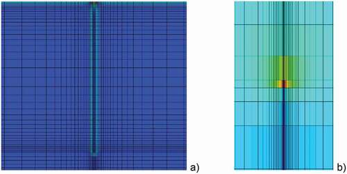
Finite element simulations were carried out using the multi-physics simulator ANSYS [24], to model the eddy current distribution, the generated Joule heating and the temperature distribution around short surface cracks. In the simulations 3D hexahedral grids with 20-node elements were used. The size of the grid was adapted to the size of the defect and to the eddy current penetration depth. Figure 1 shows two examples, how the grid is adapted around the crack tip in the depth (Figure 1a) and at the surface (Figure 1b). Additionally, close to the crack line the size of the grid is exponentially reduced. On the other hand, far away from the crack the grid size is increased, in order to optimise the necessary simulation capacities. Especially in the case simulating the eddy current heating, it is important to have a grid size, which is able to resolve the rapid changes in the eddy current density in the range of the penetration depth.

Figure 1. Gridding around a crack with 1 mm depth and 5 mm length in close-up, by simulating the Joule heating in ferro magnetic steel. a: cross-section through the middle of the crack; at the surface, at the end of the crack and close to the crack line the grid size is strongly reduced. b: Gridding at the surface around the crack tip; high grid density is applied around the crack line and around the crack tip, where a heating hot spot occurs

In the first step of the simulation the eddy current distribution and the Joule heating is calculated. The electromagnetic part of the model consists of about 300,000 elements, from which 130,000 model the sample, 20,000 the induction coil and 150,000 the surrounding air. One single straight line coil placed above the work-piece is modelled, generating an approximately homogeneous magnetic field around the crack. In the second step the heat flow is simulated. The thermal modelling was only performed for the work-piece, while the elements of the coil and the air were not included in the thermal calculation. The heating pulse and the cool-down without heating was simulated in 30 time steps. It has been observed that a higher resolution in the time is not necessary, its effect was negligible small. On the other hand, in the measurements the number of the recorded images n is important, as the noise in the phase image is reduced by $\sqrt{n}$ [23].

Figure 2 compares results for austenitic and for ferro-magnetic steel for an excitation frequency of 200 kHz. The simulated crack is l = 10 mm long and d = 1 mm deep. As the eddy current penetration depth in ferro-magnetic steel (δ = 0.034 mm) is very small compared to the crack depth, the eddy currents follow the line of the crack, see Figure 2a. The whole crack side is selectively heated, causing a higher temperature along the line of the crack. Additionally, around the tip of the crack a high current density occurs, hence here a hot spot can be observed in the temperature image, see Figure 2b [20].

Figure 2. Magnitude of the magnetic field (a, c) around a 10 mm long and 1 mm deep crack; and the temperature distribution after 0.1 s inductive heating pulse with 200 kHz excitation frequency (b, d). Figs. a and b are calculated for ferro-magnetic steel; c and d for austenitic steel. The images show only the half of the model in order to see also the distribution below the surface in the middle of the crack [20]

In the austenitic steel for the same excitation frequency the eddy current penetration depth is larger than the crack depth (δ = 1.35 mm, d = 1 mm). The current lines are deflected by the surface cracks (see Figure 2c), therefore the current density at the surface close to the crack line is reduced and the Joule heating and the temperature are less in the vicinity of the crack than at the faultless surface, see Figure 2d. But around the crack tip at the surface the same phenomena can be observed as for ferro-magnetic steel: the eddy current flows around the crack tips, causing higher current density and higher Joule heating in the vicinity of the crack tips, and hot spots occur in the temperature distribution.

Figure 3a and 3b show the temperature distribution at the surface for the same models as Figure 2. The magnetic field lies in the x-direction, and the eddy currents flow perpendicular to it in the y-direction. It is well to observe that in the case of ferro-magnetic steel in the mid of the crack the temperature is higher than at the sound surface far away from the crack. On the other hand, in the case of the austenitic steel the temperature is less in this region.

Figure 3. Temperature distribution after 0.1 s heating around a 10 mm long and 1 mm deep crack in ferro-magnetic steel (a) and in austenitic steel (b); phase images for the same cracks: (c) in ferro-magnetic steel and (d) in austenitic steel; phase images for a short crack with 2 mm length and 1 mm depth in ferro-magnetic steel (e) and in austenitic steel (f) [20]

In the mid of the crack the eddy current flows below the crack. But in the vicinity of the crack tips the currents flow close to the surface around the tip, causing a higher eddy current and Joule heating density in this region. In the corresponding phase images (Figure 3c and in Figure 3d) the crack tips have the highest phase values, because the temperature during the heating increases most rapidly in the vicinity of the crack tips and in the cool-down phase the temperature decreases most rapidly here. In the mid part of the cracks the same phase distribution can be observed as for long cracks. This is only valid, if the crack is not too short. In the case of shorter cracks, as shown in Figure 3e and 3f for 2 mm long cracks, the hot spots at the crack tips affect the phase distribution also in the middle of the crack, and in both cases, for ferro-magnetic and austenitic steel, the phase value in the middle is less than at the sound surface.

4. Influence of crack length

In Figure 4 simulation results for different crack lengths in the range of 1 mm up to 12 mm are depicted. In the phase profiles along the crack lines the hot spots at the crack ends are well visible for both materials. In these hot spots additional heat is generated, which flows to the surrounding region, causing there a slower temperature decrease than at the defect-free surface. This heat accumulation becomes visible due to a low phase value in the phase image. If the crack length is shorter than this affected range around the crack tip, then the phase value in the middle of the crack is also influenced by the heat flow from the crack tips and the phase value becomes different from the value which could be observed for a long crack. It depends on different parameters, for which crack length the phase value in the mid position of a short crack is the same as for a long crack, as e.g.:

• Heating pulse duration;

• Thermal diffusivity of the material;

• Crack depth.

Figure 4. Phase profiles along the crack calculated for different crack lengths; heating pulse = 0.1 s, crack depth = 1 mm, in ferro-magnetic steel (a), austenitic steel (b). In both figures the line belonging to the shortest crack length, where the phase value in the mid of the crack is approximately equal to the phase value of a very long crack, is plotted as a thick black line

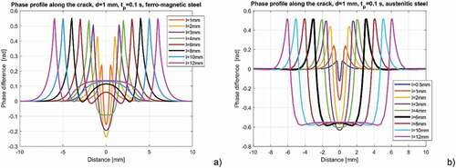
But the range of this critical crack length is around 6–10 mm, and this is valid for both types of steel material. In the case of a 1 mm deep crack in ferro-magnetic steel with 0.1 s heating pulse the crack length 8 mm shows the same behaviour in the middle of the crack as for a long crack. For austenitic steel in the case of 1 mm deep crack and 0.1 s heating pulse duration the limit is about 6 mm length. These two curves are plotted with a thicker black line in Figure 4.

5. Influence of crack depth

The deeper a crack is, the larger obstacle it presents for the eddy currents and for the heat flow. Therefore, the phase contrast around a crack is increasing with the crack depth [14]. Figure 5 compares the phase profiles across and along the cracks for different crack depths. The length of all these cracks is 10 mm. In Figure 5a and 5b, it can be noticed that not only the phase contrast in the central position but also the phase values at crack tips increase with the crack depth.

Figure 5. Phase profiles along the crack calculated for different crack depths; heating pulse = 0.1 s, crack length = 10 mm, in ferro-magnetic steel (a), in austenitic steel (b). In figures c and d phase profiles across the cracks in the mid positions are compared to the ones across long cracks, the latter ones are plotted by dashed lines; Figures e and f show the phase plotted as a surface with the definitions for the profiles: red lines mark the phase profile along the crack and yellow lines show for the phase profile across the crack in its middle

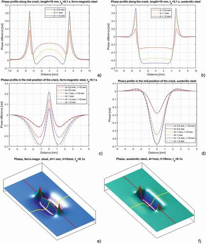
In Figure 5c and 5d, the phase profiles across the 10 mm long cracks are plotted together with the phases calculated for long cracks. The main difference in the modelling is, that long cracks can be simulated in a 2D model, in a cross-section across the crack. For short cracks the simulation model has to be setup in 3D, in order to consider the length of the crack and the flow around the crack tips. As in Figure 5c and 5d can be seen, for the crack with a length of 10 mm the phase in the mid position of the crack is almost identical to the long ones.

In Figure 5e and 5f the phase distribution is plotted as a surface, with a red and with a yellow line, which demonstrates the definitions of the two kinds of profiles: along and across the crack.

5.1. Phase contrast in austenitic steel

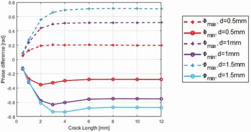
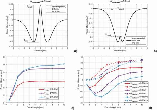
In the austenitic steel a crack can be characterised by two phase values: the maximum phase value at the crack tip (Φ_max) and the minimum phase value at the centre of the crack (Φ_min). Figure 6 shows how these two phase values are changing with the crack depth and length. For better comparison phase differences are depicted in the figure, and the difference to the phase of the defect-free surface is plotted. It can be well observed that the deeper the crack is, the larger are both phase differences Φ_max and |Φ_min|. For short cracks up to about 2 mm length both Φ_max and |Φ_min| are less than those for longer cracks. Between 2 and 6 mm length it is a transition range, and cracks with 6 mm length or longer show the same phase differences Φ_max and Φ_min independently on the crack length. This statement is valid for all the three investigated crack depths from 0.5 mm up to 1.5 mm.

Figure 6. Phase at the crack tip (Φ_max) and phase at the middle of the crack (Φ_min) depending on the length of the crack, calculated for three different crack depth values. For the simulations austenitic steel parameters were used, heating pulse = 0.1 s, excitation frequency = 200 kHz. In the diagram the phase difference to the phase at the sound surface is plotted

5.2. Phase contrast in ferro-magnetic steel

In the case of austenitic steel, the eddy current penetration depth is larger or comparable to the investigated crack depth values. Hence, there is a maximum phase value at the crack tip, and a negative minimum phase value at the crack position. Also in ferro-magnetic steel the maximum phase value occurs at the tip of the crack. But the phase distribution around the line is more complex, as it can be seen in Figure 5c. Since the crack is selectively heated, a high temperature and a high phase value occurs along its line. But in a distance of about 1.3 mm from the crack line the phase has a minimum value. This is only valid for longer cracks, for short cracks the crack line itself does not show a higher phase value, as it can be noticed by comparing Figure 3c and Figure 3e. Therefore, the phase contrast, which is relevant for the detection of a crack, is defined in two ways, as it is depicted in Figure 7a and 7b:

(5) ${\mathrm{\Phi }}_{contrast1}={\mathrm{\Phi }}_{crack}-{\mathrm{\Phi }}_{min}$(5)

(6) ${\mathrm{\Phi }}_{contrast2}={\mathrm{\Phi }}_{crack}-{\mathrm{\Phi }}_{sound}$(6)

Figure 7. A and b show the two different ways to define the phase contrast for ferro-magnetic steel; c: Φ_max at the crack tip calculated for three different crack depth values and plotted in dependency of the crack length; d: both phase contrasts according to Eqs.5(5) ${\mathrm{\Phi }}_{contrast1}={\mathrm{\Phi }}_{crack}-{\mathrm{\Phi }}_{min}$(5) and 6(6) ${\mathrm{\Phi }}_{contrast2}={\mathrm{\Phi }}_{crack}-{\mathrm{\Phi }}_{sound}$(6) , for the same cracks as in fig.c; the simulations were calculated for heating pulse = 0.1 s and excitation frequency = 200 kHz

Depending on which of these contrasts the absolute value is larger, it will be noticed in an image and used to characterise the crack:

(7) $\begin{array}{rl}& if\left|{\mathrm{\Phi }}_{contrast1}\right|>\left|{\mathrm{\Phi }}_{contrast2}\right|,then{\mathrm{\Phi }}_{contrast}={\mathrm{\Phi }}_{contrast1}\\ & else{\mathrm{\Phi }}_{contrast}={\mathrm{\Phi }}_{contrast2}\end{array}$(7)

5.3. Comparison of phase contrast for ferro-magnetic and austenitic steel

Comparing Figure 6 for austenitic steel and Figure 7 for ferro-magnetic steel, the following points can be recognised:

• Short cracks with length of 0.5–2 mm look similar for both materials: both hot spots at the end of the cracks are visible and between them the phase value is negative. This can be also seen in Figure 3e and 3f.

• Cracks with 2–6 mm length show also similar patterns with two hot spots and negative phase values between them. But this negative value in the middle of the crack in absolute value is larger than for significantly longer cracks. The additional heat flow from the hot spots to their vicinity causes there a heat accumulation and the temperature decreases slower than at the sound surface. Consequently, at the position of the crack the phase value becomes lower.

• Cracks longer than 6–8 mm have the same phase contrast in the middle position as long cracks, the length of the crack has no effect on the phase contrast.

• The deeper the crack is, the larger is the phase value Φ_max at the hot spot. A crack represents a large obstacle for the eddy currents, causing a large amount of additional Joule heating in the vicinity of the crack ends, which further means an increased phase value at the tips.

• Φ_max is increasing up to a crack length of about 2–4 mm, for longer cracks Φ_max shows a constant value.

6. Influence of the crack profile

All the simulated defects presented until now have a rectangular shape inside the material. Natural, fatigue cracks have usually a different profile, which is closer to a half-penny shape instead of a rectangular one [19]. Usually the crack does not penetrate abruptly to the maximum crack depth, but it starts slowly with a lower slope until achieving the deepest point. In order to analyse the effect of the crack profile further simulations were calculated for cracks with trapezoid shape. Figure 8 and Figure 9 show phase images, where the crack length at the surface is 10 mm, but inside the material the length is shorter. The crack ends penetrate slanted into the material, having a trapezoid shape, see Figure 8c.

Figure 8. Simulation results for 10 mm long and 1 mm deep vertical cracks in ferro-magnetic steel with different cross-section profiles; top a: rectangular profile, l_depth = 10 mm, bottom a: l_depth = 5 mm, fig. b: comparing the profiles along the crack; fig. c: sketch of the trapezoid shaped crack with the length definitions

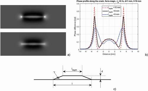
Figure 9. Simulation results for 10 mm long and 1 mm deep vertical cracks in austenitic steel with different cross-section profiles; top a: rectangular profile, l_depth = 10 mm, bottom a: l_depth = 5 mm, fig. b: comparing the profiles along the crack

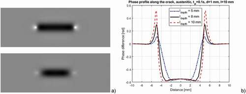
Comparing the phase images (Figures 8a and 9a) and the phase profiles along the crack line (Figures 8b and 9b), it can be observed that the ‘hot spots’ at the crack tips are much less dominant for the trapezoid shaped cracks than for the rectangular ones. In Figures 8b and 9b it can be noticed, that the smaller the angle γ, the less is the phase value at the hot spot. Figure 10 compares the phase values for ferro-magnetic and for austenitic steel, assuming a rectangular and a trapezoid shaped crack. For these calculations γ = 45° was taken, if the crack was at least 4 times longer than its depth, otherwise a steeper angle:

(8) $\begin{array}{rl}& ifl\ge 4d,then{l}_{depth}=l-2d\left(\gamma ={45}^{\circ }\right)\\ & else{l}_{depth}=l/2\left(\gamma =arctan\left(\frac{d}{l/4}\right)\right)\end{array}$(8)

Figure 10. Phase maximum, phase minimum and contrast for ferro-magnetic (a) and for austenitic (b) steel, comparing cracks with rectangular shape (l_depth = l_surf) and cracks with trapezoid shape (l_depth < l_surf)

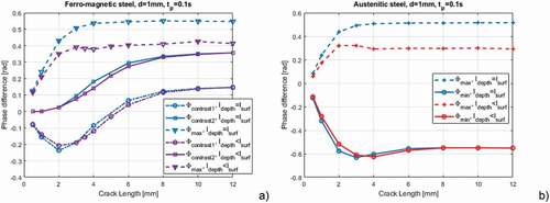
In Figure 10 it can be observed for both materials, that the phase at the mid part of the crack is hardly affected by the shape of the defect. Φ_min for the austenitic steel and both Φ_contrast1 and Φ_contrast2 are almost the same for the rectangular and for the trapezoid shape. On the other hand, the phase value at the crack tip Φ_max is strongly decreasing with the angle γ. This dependency of Φ_max on the phase profile is important to consider, as this means that the phase value at the crack tip cannot be used for estimation of the depth of the crack. This phase value is only characteristic for the angle γ, how the crack penetrates into the material.

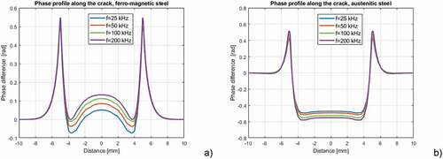
7. Influence of the excitation frequency

The excitation frequency determines the eddy current penetration depth according to Eq.1(1) $\delta =\sqrt{\frac{1}{\pi {\mu }_0{\mu }_r\sigma f}}$(1) , larger frequency resulting a smaller penetration depth. On the other hand, the total Joule heating induced in the sample is proportional to $\sqrt{f}$, assuming that the induction generator can generate at each frequency the same electrical current in the induction coil [25]. But induction generators work only in a specified frequency range. There are generators, which work at the resonance frequency of their circuit, consisting of internal capacities and the external induction coil. For this kind of generator it is very tedious to change the resonance frequency, as capacities inside the generator has to be exchanged. Other type of generator works with pulse width modulation, where it is easier to modify the working frequency in a specified range. Figure 11 shows phase profiles simulated for different excitation frequencies. It can be seen that in the case of austenitic steel, the influence of the frequency on the phase contrast is rather small. In the case of ferro-magnetic steel a slight increase of the phase in the centre of the crack can be observed, if the excitation frequency is increased.

Figure 11. Phase profiles along the crack calculated for different excitation frequencies, crack depth = 1 mm, crack length = 10 mm, in ferro-magnetic steel (a) and in austenitic steel (b)

8. Influence of the heating pulse duration

The eddy current distribution is disturbed by a crack causing an inhomogeneous Joule heating and an inhomogeneous temperature distribution. But the heat flow starts to equalise this inhomogeneity even during the heating pulse. The longer the heating pulse, the more this temperature difference diminishes. Figure 12 compares the phase profiles for different heating pulse durations. It can be noticed in Figure 12a and b how the heat diffuses from the hot spots away in the vicinity of the crack tips. For longer heating pulse the intensity of the peak is reducing and the size of the hot spot is increasing.

Figure 12. Phase profiles along the crack calculated for different heating pulse durations, crack depth = 1 mm, crack length = 10 mm, in ferro-magnetic steel (a) and in austenitic steel (b); phase profiles across the mid of the crack in ferro-magnetic steel (c) and austenitic steel (d)

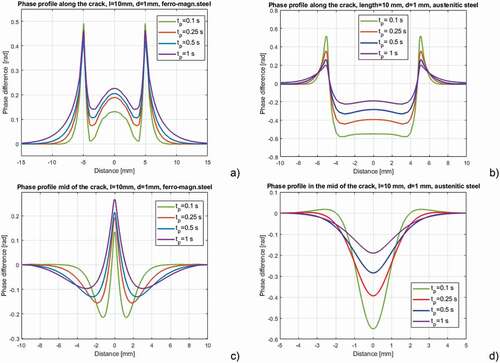
In the case of ferro-magnetic steel, the phase contrast at the crack position is less affected by the pulse length than it is the case for the austenitic steel. But the signal around the crack becomes wider due to the heat diffusion, and the width of the effected range around the crack can be estimated by the thermal diffusion length, see Eq.2(2) $d_{th}=2\sqrt{\kappa t}$(2) . Therefore, if more defects lying close to each other, which should be separately detected, then a short heating pulse is recommended, otherwise the signals of the separate cracks influence each other.

In the case of austenitic steel, the phase contrast Φ_min at the mid of the crack is strongly decreasing with longer pulse duration. In a non-magnetic material the efficiency of the inductive heating is low, as the generated Joule heating is proportional to $\sqrt{{\mu }_r}$ [25]. In order to achieve a higher temperature increase, an idea could be to increase the heating pulse length. On the other hand, as it can be seen from Figure 12b and d, with increasing pulse length the phase contrast decreases, and the detectability becomes less. Since due to the short pulses the phase contrast remains high, another possibility is to apply multiple short pulses [23]. With increasing the number of applied pulses the noise in the image can be reduced [23].

9. Influence of the inclination angle of the crack

All the cracks investigated in the previous sections were vertical cracks, that means the crack was penetrating under 90° into the material. In many cases, cracks have an inclination angle, which has also influence on the temperature and on the phase distribution observed at the surface. Figure 13 shows phase distribution around four cracks with different angles in ferro-magnetic steel and for Figure 14 the same cracks were modelled but in austenitic steel. Due to the difference in the angle on both sides of the crack, the phase distribution becomes asymmetric. At the side of the crack with the small angle the heat is trapped longer, therefore at this side the phase has a lower phase value. This behaviour is identical to the one observed for long cracks [14], but for short cracks additionally hot spots at the crack tips occur.

Figure 13. Phase distribution for 1 mm deep and 6 mm long cracks in ferro-magnetic steel with different inclination angles below the surface: 90° (a), 60° (b), 45° (c), 30° (d) between crack and surface. The images show 12 × 12 mm² area around the cracks and all the images have the same scaling, corresponding to the colorbar at the right side

Figure 14. Phase distribution for 1 mm deep and 6 mm long cracks in austenitic steel with different inclination angles below the surface: 90° (a), 60° (b), 45° (c), 30° (d) between crack and surface. The images show 12 × 12 mm² area around the cracks and all the images have the same scaling, corresponding to the colorbar at the right side

10. Influence of the angle between crack line and coil

In the previous sections the induced eddy currents were applied perpendicular to the crack line. In this case the disturbance caused by a crack is the largest, resulting the largest contrast between the crack and the defect-free surface. But if cracks can lie in any direction at the surface, then it is not possible to maintain always this optimal inspection setup.

Figures 15 and 16 demonstrates how the angle between the crack line and the induced eddy currents influences the phase distribution. The so-called ‘butterfly’ pattern around the crack becomes asymmetric, the hot spots are pushed a bit away from the crack tip and the low phase value region along the crack line varies in its intensity. If the angle is less than 90°, then the phase contrast decreases. In the case when the crack is parallel to the eddy current line, then the crack does not deflect the eddy currents, therefore the crack cannot be detected. To overcome this direction dependency of the crack detection, it has been suggested to use two induction generators inducing magnetic fields perpendicular to each other with different excitation frequencies, causing a rotating magnetic field [9,18].

Figure 15. Phase distribution for 1 mm deep and 6 mm long vertical cracks in ferro-magnetic steel with different angles between the crack lines and the induced eddy currents: 90° (a), 60° (b), 45° (c), 30° (d). The images show 12 × 12 mm² area around the cracks and all the images have the same scaling, corresponding to the colorbar at the right side

Figure 16. Phase distribution for 1 mm deep and 6 mm long vertical cracks in austenitic steel with different angles between the crack lines and the induced eddy currents: 90° (a), 60° (b), 45° (c), 30° (d). The images show 12 × 12 mm² area around the cracks and all the images have the same scaling, corresponding to the colorbar at the right side

It is notable, that a dependency of the detectability on the crack orientation is also the case for other magnetic induced NDT testing methods, as e.g. for magnetic particle testing. A crack can be only detected, if the magnetic field is disturbed by the crack. Hence for an entire inspection of a surface with any crack orientation two magnetic fields with 90° to each other have to be applied. This is done either by two inspection steps after each other or by applying magnetic excitations with different frequencies.

Figures 17 and 18 show how the phase pattern changes for an inclined crack when the angle between the crack line and induced eddy currents varied from 90° to 30°. All the cracks have 30° angle to the surface. Figure 17 shows the phase distribution simulated for ferro-magnetic and Figure 18 for austenitic steel. The asymmetric phase distribution at the sides of the crack can be observed and the phase contrast decreases strongly with decreasing angle between the crack line and the eddy currents.

Figure 17. Phase distribution for 1 mm deep and 6 mm long cracks in ferro-magnetic steel, all the cracks have 30° inclination angle to the surface and different angles between the crack lines and the induced eddy currents: 90° (a), 60° (b), 45° (c), 30° (d). The images show 12 × 12 mm² area around the cracks and all the images have the same scaling, corresponding to the colorbar at the right side

Figure 18. Phase distribution for 1 mm deep and 6 mm long cracks in austenitic steel, all the cracks have 30° inclination angle to the surface and different angles between the crack lines and the induced eddy currents: 90° (a), 60° (b), 45° (c), 30° (d). The images show 12 × 12 mm² area around the cracks and all the images have the same scaling, corresponding to the colorbar at the right side

It is to notable that Figure 17a is identical to Figure 13d and Figure 18a is identical to Figure 14d. Furthermore, Figure 13a is identical to Figure 15a and Figure 14a is identical to Figure 16a, but the scaling of the images was selected in such a way that for the four images shown in one figure the scaling is always the same and optimal for these corresponding four images.

11. Experimental results

The main emphasis of this paper is to investigate the influence of different parameters on the inductive thermography results using finite element simulation models. In this section couple of experimental results are presented to show the good correspondence between the simulated and the experimental results.

In the experiments a 10 kW induction generator was used and the excitation frequency was 200 kHz. The sample is placed in the middle of a Helmholtz coil [9] and the infrared camera records the surface temperature from the top. The infrared camera has a cooled InSb detector and it is sensitive in the 1.5–5.1 µm mid-IR range. The recording frequency was 380 Hz.

In Figure 19a, the sample is ferro-magnetic and the crack length is about 12 mm long and has approximately a depth of 1 mm [20]. In Figure 19b the sample is austenitic steel and the fatigue crack has approximately a half-penny shape and a depth of 1.5 mm [19]. Both cracks are natural cracks and not visible to naked eye due to their opening just in µm range. It was not necessary to blacken the surface to increase the emissivity, the measurements were carried out at the partially shiny surface. In both cases the cracks can be made well visible using inductive thermography and due to the phase calculation the signal-to-noise ratio in significantly higher, than in a temperature image. The hot spots at the end of the cracks can be well recognised, and measuring their distance the crack length can be determined. Comparing the phase value in the mid of the crack, the depth can be estimated as well. It is noticeable, that in the ferro-magnetic steel along the crack the phase value is higher than at the sound surface, similarly to the simulations. On the other hand, in the austenitic steel, due to the larger eddy current penetration depth, the phase value along the crack is less than at the sound surface, as it has been predicted by the simulations.

Figure 19. a: Phase image of a 12 mm long crack in ferro-magnetic steel sample after 0.1 s heating pulse duration; b: phase image of a 6 mm long fatigue crack in austenitic steel after 0.5 s heating pulse duration [19,20]

Figure 20 shows two phase images of ferro-magnetic steel sample with artificial defects. It was manufactured by Direct Metal Laser Sintering. The artificial cracks have an opening of 0.25–0.3 mm, therefore their lines are well visible in the images. Figure 20a shows the CAD design of the sample, the 1st row of the cracks have a length of 10 mm and the 2nd one 5 mm. The depth in the 1st row is 1 and 0.6 mm and the 2nd and 4th cracks from the left side have an inclination angle. In the 2nd row all the cracks are vertical, and their depth is 0.4, 0.6, 0.8 and 1 mm [18]. In Figure 20b the phase image is depicted, when the induced eddy currents are perpendicular to the crack lines, in Figure 20c they are enclosing 45°. The results as predicted by the simulations can be well observed:

• Hot spots occur at the end of the crack tips;

• The phase contrast is increasing with the crack depth, see Figures 20b, 2nd row;

• The phase is asymmetric for inclined cracks, see Figures 20b, 2nd and 4th cracks in the 1st row;

• The phase pattern is shifted along the crack line and its intensity is less, when the crack line and the eddy current direction encloses an angle less than 90°, see Figure 20c.

Figure 20. A: CAD drawing of the sample with artificial cracks; phase images after 0.3 s heating pulse, the induced eddy currents are perpendicular to the crack lines (b) and enclose 45° (c)

12. Summary

Finite element simulation results were presented for short surface cracks in the range of 1–14 mm length, and they were investigated in ferro-magnetic as well as in austenitic, non-magnetic steel. It was investigated how different parameters, as material parameters, crack geometry and parameters of the inspection setup influence the results. The simulated temperature sequence during and after the short heating pulse was transformed to a phase image. In earlier publications [14,18] the phase contrast was investigated for long cracks and how this contrast can be used for estimation of the crack depth. In this actual paper the main goal was to study, whether this estimation can be also applied for short cracks and up to which length is this valid.

The simulation results show that short cracks can be well detected from the hot spots at the crack tips. The phase value between the hot spots for very short cracks (length appr. 1–2 mm) is in both materials lower than at the sound surface. If the crack is longer than about 8−10 mm then the phase value in the mid position of the crack is similar to the phase of long cracks, which can be modelled with 2D simulations or calculated analytically [14]. Therefore, the phase values at the mid position of cracks, which are longer than 8 mm, can be used also for the depth estimation, as it is described in [14].

The phase value at the hot spots is not appropriate for depth estimation. The crack profile, whether it is rectangular, half-penny or trapezoid shaped, has a strong influence on the intensity of the hot spot, and this effect is more significant than the dependency on the crack depth.

A surface crack disturbs the eddy current flow causing an irregular Joule heating distribution in the vicinity of the crack. The differences in the heat distribution are equalised by the heat diffusion. Hence a shorter heat pulse results in a higher phase contrast. The longer the heating pulse is, the more time expires during the measurement and the local disturbance caused by the crack diminishes during this time.

If a crack does not penetrate vertically into the surface, but having an inclination angle, then this can be observed at the surface by the asymmetric phase distribution. At the flank with the acute angle the heat accumulates and the temperature is kept longer, causing a low phase value.

In the current paper only some experimental results were presented in order to demonstrate the capability of the inductive thermography to detect short surface cracks. Several other experimental results can be found in the referenced publications [12,14,18].

Acknowledgments

This project has received funding from the Clean Sky 2 Joint Undertaking (JU) under grant agreement Nº. 101007699. The JU receives support from the European Union’s Horizon 2020 research and innovation programme and the Clean Sky 2 JU members other than the Union.

Disclosure statement

No potential conflict of interest was reported by the author.

Data Availability Statement

The infrared measurement files which were evaluated to obtain Figure 19a, Figure 20b and 20c are openly available at https://zenodo.org/record/5037199

Additional information

Funding

This work was supported by the CleanSky2 [101007699].

Notes on contributors

Beate Oswald-Tranta

Beate Oswald-Tranta received her MS in electrical engineering. She made her PhD at the area of solid state physics, modelling and measuring of semiconductor structures for infrared detection. Since 2003 she works at the Chair for Automation, University of Leoben. Her research fields are automated non-destructive testing, thermography and image processing.

References

- Kremer KJ, Kaiser W, Möller P. Das Therm-O-Matic-Verfahren - ein neuartiges Verfahren für die Online-prüfung von Stahlerzeugnissen auf Oberflächenfehler. Stahl und Eisen. 1985;105:39–44.
- Maldague X. Infrared and Thermal Testing, Nondestructive testing handbook, Vol. 3.In: Maldague XPV, Moore PO. Columbus (OH): American Society for Nondestructive Testing (ASNT); 2001. p. 307–342, Available from: http://www.asnt.org
- Riegert G, Zweschper T, Busse G. Lockin thermography with eddy current excitation. QIRT J. 2004;1(1):21–32.
- Riegert G, Gleiter A, Busse G. Potential and limitations of eddy current lockin-thermography. Defense Secur Symp. 2006;6205. DOI:https://doi.org/10.1117/12.662716
- Oswald-Tranta B. Thermoinductive investigations of magnetic materials for surface cracks. QIRT J. 2004;1(1):33–46.
- Vrana J, Goldammer M, Baumann J, et al. Mechanism and models for crack detection with induction thermography. AIP Conf Proc. 2008;1706:475–482.
- Wilson J, Tian GY, Abidin IZ, et al. Modeling and evaluation of eddy current stimulated thermography. J Nondestr Test Eval. 2010;25(3):205–218.
- Netzelmann U, Walle G. Induction thermography as a tool for reliable detection of surface defects in forged components. In Proceedings of the 17th World Conference on Non Destructive Testing, Shanghai, China, 25–28 October 2008.
- Oswald-Tranta B, Sorger M. Localizing surface cracks with inductive thermographical inspection: from measurement to image processing. QIRT J. 2011;8(2):149–164.
- Netzelmann U, Walle G, Ehlen A, et al. NDT of railway components using induction thermography. AIP Conf Proc. 2016;1706:1–8.
- Wilson J, Tian G, Mukriz I, et al. PEC thermography for imaging multiple cracks from rolling contact fatigue. NDT E Int. 2011;44(6):505–512.
- Tuschl C, Oswald-Tranta B, Eck S. Inductive thermography as non-destructive testing for railway rails. Appl Sci. 2021;11(3):1003.
- Abidin IZ;, Tian GY, Wilson J, et al. Quantitative evaluation of angular defects by pulsed eddy current thermography. NDT E Int. 2010;43(7):537–546.
- Oswald-Tranta B. Induction thermography for surface crack detection and depth determination. Appl Sci. 2018;8(2):257
- Srajbr C. Induction excited thermography in industrial applications”, In Proceedings of the 19th World Conference on Non-Destructive Testing, Munich, Germany, 13–17 June 2016.
- Netzelmann U, Walle G, Lugin S, et al. Induction thermography: principle, applications and first steps towards standardization. QIRT J. 2016;13(2):170–181.
- DIN 54183:2018–02. Non-destructive testing-Thermographic testing- Eddy-current excited thermography; Available online: https://www.din.de (cited Jan 2018)
- Oswald-Tranta B. Investigations for determining surface crack depth with inductive thermography Proc. of the 19th World Conference on Non-Destructive Testing, Munich, Germany, 13–17 June 2016.
- Oswald-Tranta B, Feistkorn S, Rössler G, et al. Comparison of different inspection techniques for fatigue cracks. in Proc. SPIE 11409, Thermosense: Thermal Infrared Applications XLII, 2020
- Oswald-Tranta B, Tuschl C. Detection of short fatigue cracks by inductive thermography, in Proc. of 15th QIRT Conf., 2020
- Oswald-Tranta B. Thermo-inductive crack detection. J Nondestr Test Eval. 2007;22(2–3):137–153.
- Oswald-Tranta B. Time-resolved evaluation of inductive pulse heating measurements. QIRT J. 2009;6(1):3–19.
- Oswald-Tranta B. Lock-in inductive thermography for surface crack detection in different metals. QIRT J. 2019;16(3–4):276–300.
- ANSYS, Inc. Available online: http://www.ansys.com (cited 2018 Jan 1).
- Oswald-Tranta B. Surface crack detection in different materials with inductive thermography, in Proc. SPIE Thermosense XXXIX, vol.10214, Anaheim, California, United States, 2017