Macroeconomic effects of global shocks in the GCC: evidence from Saudi Arabia

ABSTRACT

We develop a quarterly macro-econometric model for the Saudi economy over the period 1981Q2-2018Q2 and integrate it within a compact model of the world economy (including the global oil market). This framework enables us to disentangle the size and speed of the transmission of growth shocks originating from the United States, China, and the world economy to Saudi Arabia, as well as study the implications of stress in global financial markets, low oil prices, and domestic fiscal adjustment on the Saudi economy. Results show that Saudi Arabia's economy is becoming more sensitive to developments in China than to shocks in the United States – in line with the direction of evolving trade patterns and China's growing role in the global oil market. A global growth slowdown (e.g. from trade tensions or geopolitical developments) could have significant implications for Saudi Arabia (with a growth elasticity of about 2½ after one year) and the oil market (reducing prices by about 5% for 0.5 percentage point reduction in global growth). We also illustrate that a 10% lower oil prices and stress in global financial markets could both have a negative effect on the Saudi economy, but given the prevailing social contract in Saudi Arabia, their impact is countered by fiscal easing. Finally, we observe that a domestic fiscal adjustment in Saudi Arabia does not show a negative impact on economic growth in the data. The impact on growth would depend upon the quality of fiscal adjustment and whether it is complemented with structural reforms.

KEYWORDS:

• Saudi Arabia
• stress in global financial markets
• international business cycle
• fiscal policy
• Global VAR

JEL CLASSIFICATIONS:

• C32
• E32
• E62
• F44
• O53

1. Introduction

Demand-driven fluctuations in oil prices, from upswings or downturns in global growth, are closely linked to changes in output and fiscal balances in the Gulf Cooperation Council (GCC).¹ This is because oil revenues constitute a major source of finance for growth and development expenditure in the GCC economies. Since mid-2014 until mid-2018, when oil prices fell by as much as 50 percent from their peak, economic growth in GCC economies plummeted to an average of 1.8 percent from about 5 percent in the preceding 5 years. Fiscal balances deteriorated and public debt levels increased across GCC economies as oil revenues fell sharply but public expenditure continued to rise. While demand for oil has been reduced by growth rebalancing in China and weak economic activity in major advanced economies, oil prices have also been affected by supply shocks such as the expansion in unconventional/shale sources of oil and gas. As one would expect in such circumstances, the rebound in oil prices from the 2014 plunge has been slow and partial, even with the OPEC restrictions on oil production during the 2017–2019 period to stabilize prices. Therefore, there is merit in examining the spillover effects of oil price shocks and growth slowdown in major economies on GCC economies as business cycles across the world continue to mature and against the backdrop of elevated public and private debt levels (United Nations, 2019).²

Loss of revenues rooted in low oil prices put limits on social spending in oil-rich countries – requiring additional efforts to achieve the Sustainable Development Goals (UNESCWA, 2017). Considering the low oil price environment before the large global fiscal support in response to Covid-19³ and the recent war in Ukraine, the GCC economies have tried to diversify their sources of income by focusing on non-oil revenues, for example through the introduction of a GCC-wide Value Added Tax (VAT) – a form of tax on goods and services – and by reducing energy subsidies. The implementation of the regional VAT is led by Saudi Arabia and United Arab Emirates; both countries introduced a 5 percent VAT on most goods and services in 2018. Bahrain followed suit in 2019. Oman took a different route and introduced excise taxes on tobacco products and sugary drinks in mid-2018 and increased corporate income taxes (World Bank, 2019). On public expenditure side, subsidies on energy products were eliminated in some countries, such as in the United Arab Emirates, while in the case of other GCC economies, they were reduced substantially. While these measures are meant to narrow fiscal deficits, they will have implications for economic growth and inflation. We, therefore, estimate the macroeconomic effects of domestic fiscal adjustments in Saudi Arabia, and qualitatively discuss the role of the composition of spending cuts or tax increases as well as structural reforms. To the extent that non-oil revenue-enhancing measures reduce distortions in the economy, they can also help with the objectives of economic diversification and improved welfare.

For the GCC economies, increasing productivity growth in the non-oil sector is key to economic diversification and improved welfare, and could lower the cost of fiscal adjustments. Currently, non-oil sectors in the GCC countries comprise of construction, hotels and restaurants, and other services – which rely on cheap labor from abroad. This is neither conducive to manufacturing growth nor helpful to high-tech industries, nor incentivizes improved education, which are essential for productivity growth and long-term development (UNESCWA, 2017). These structural rigidities may also limit the scope for non-oil revenue mobilization and could adversely affect the export competitiveness of the non-oil sectors (Elbadawi & Soto, 2011; Nabli et al., n.d.). Several GCC economies recognize these challenges, and in their ambitious Vision documents, plan to engage in structural reforms, scale up investment, and improve their sovereign debt management. Saudi Arabia, the biggest oil producer in the GCC, is among the leaders in the region in structural reforms consistent with its new national vision 2030.⁴ Whether these reforms would lead to private investment by non-residents; and how they would contribute to diversifying exports are yet to be assessed.

There are also considerations to align exchange rates with macroeconomic fundamentals and desirable policy settings, diversify export baskets, improve competitiveness, and move toward a single currency in the GCC economies. Several countries in the GCC have faced a challenging situation in the aftermath of drop in oil prices between 2014 and 2018 as the pegs versus US dollar⁵ came under pressure owing to fiscal and current account deficits, and substantial reductions in foreign exchange reserves. The fluctuations in the balance of payment positions of oil exporting countries, linked to oil prices, puts pegged exchange rates under pressure periodically. This necessitates assessing the impact of external shocks or domestic policy changes on output, inflation, and fiscal balances (Bhanumurthy & Sarangi, 2019).

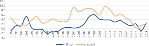
This paper focuses on Saudi Arabia as the largest economy in the GCC. The decline in oil price between mid-2014 and mid-2018 had a significant impact on growth and fiscal balances of Saudi Arabia. Economic growth fell from an average of 5.3 percent between 2010 and 2014 to 1.7 percent over 2015–2017. The fiscal balance deteriorated significantly and registered a deficit of −17 percent of GDP in 2014, before improving to −9 percent in 2017, while current account remained in deficit during 2015 and 2016. Economic growth picked up slowly and reached 2.5 percent in 2018, led by improvements in the oil sector as well as the non-oil sector. The non-oil output growth was 2.2 percent in 2018, after a long decline from 9.5 percent in 2010 to 0.2 percent in 2016 (Figure 1). While oil output tracks oil prices, inflation reflects the developments in the non-oil output (Figure 2). Studying the impact of oil price shocks, slowdown in global economic growth and stress in global financial markets (external shocks), as well as fiscal policy changes (as the key policy tool domestically) would help drawing implications for economic growth and performance of the non-oil output.

Figure 1. Oil and non-oil sector growth in Saudi Arabia. Source: General Authority of Statistics, Saudi Arabia.

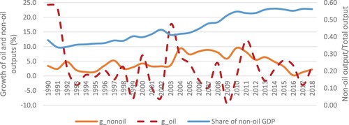
Figure 2. Inflation rate and growth of non-oil output in Saudi Arabia. Source: General Authority of Statistics, Saudi Arabia.

To this end, we build a Global VAR (GVAR) model to disentangle the size and speed of the transmission of growth shocks originating from China, the United States, or the world economy to Saudi Arabia, as well as to study the implications of stress in global financial markets, lower oil prices, and a domestic fiscal tightening on the Saudi economy. Our approach uses a dynamic multi-country framework for the analysis of the international transmission of shocks and is based on the models developed Cashin et al. (2014), Cashin et al. (2016), Cashin et al. (2017b) and Mohaddes and Pesaran (2016). The framework comprises 33 country/region-specific models. These individual models are solved in a global setting where core macroeconomic variables of each economy are related to corresponding foreign variables (constructed exclusively to match the international trade pattern of the country under consideration). The model has both real and financial variables: real GDP, inflation, primary balance to GDP ratio, public debt to GDP ratio, real exchange rate, short and long-term interest rates, an index of financial market stress, and the price of oil. This framework can account for various transmission channels, including not only trade relationships but also financial and commodity price linkages, see Dees et al. (2007). The GVAR has several advantages over a simple VAR for the Saudi economy alone. First, external shocks can originate from any country or region (e.g. US, China, and euro area as opposed to the ‘rest of the world’ as a block). Second, oil prices are determined endogenously with feedback effects from macroeconomic developments in the world economy (rather than exogenously). Third, the Generalized Impulse Response Functions not only account for direct effects of shocks on the Saudi economy but also indirect effects through third markets.

The rest of this paper is organized as follows. Section 2 describes the Global VAR (GVAR) methodology, outlines our modelling choices, and presents the country-specific estimates and tests. Section 3 studies spillovers of various shocks to the Saudi economy as well as commodity markets. Finally, Section 4 offers some concluding remarks.

2. Modelling the global economy

We employ the GVAR methodology to analyze the international macroeconomic transmission of shocks with a focus on the Saudi Arabian economy. This framework takes into account both the temporal and cross-sectional dimensions of the data; real and financial drivers of economic activity; interlinkages and spillovers that exist between different regions; and the effects of unobserved or observed common factors (e.g. commodity prices and financial risk).⁶ This is crucial as the impact of shocks cannot be reduced to a single country but rather involves multiple regions, and this impact may be amplified or dampened depending on the degree of openness of the countries and their trade structure. Before describing the data and our model specification, we provide a short exposition of the GVAR methodology.

2.1. The global VAR (GVAR) methodology

The Global VAR methodology consists of two main steps. First, each country is modeled individually as a small open economy (except for the United States) by estimating country-specific vector error correction models in which domestic variables are related to both country-specific foreign variables and global variables that are common across all countries (such as oil prices and an index of financial stress, FSI). Second, a global model is constructed combining all the estimated country-specific models and linking them with a matrix of predetermined cross-country linkages. More specifically, we consider $N+1$ countries in the global economy, indexed by $i=0,1,\dots ,N$. Except for the United States, which we label as $0$ and take to be the reference country; all other $N$ countries are modelled as small open economies. This set of individual VARX* models is used to build the GVAR framework. Following Pesaran et al. (2004) and Dees et al. (2007), a VARX*$(p_i,q_i)$ model for the $i$th country relates a $k_i\times 1$ vector of domestic macroeconomic variables (treated as endogenous), $x_{\mathrm{it}}$, to a $k_i^{\ast }\times 1$ vector of country-specific foreign variables (taken to be weakly exogenous), $x_{\mathrm{it}}^{\ast }$: (1) ${\mathrm{\Phi }}_{\mathrm{i}}(L,p_i)x_{\mathrm{it}}=a_{\mathrm{i}0}+a_{\mathrm{i}1}\mathrm{t}+{\mathrm{\Lambda }}_{\mathrm{i}}(L,q_i)x_{\mathrm{it}}^{\ast }+u_{\mathrm{it}},$(1) for $t=1,2,\dots ,T$, where $a_{\mathrm{i}0}$ and $a_{\mathrm{i}1}$ are $k_i\times 1$ vectors of fixed intercepts and coefficients on the deterministic time trends, respectively, and $u_{\mathrm{it}}$ is a $k_i\times 1$ vector of country-specific shocks, which we assume are serially uncorrelated with zero mean and a non-singular covariance matrix, ${\mathrm{\Sigma }}_{\mathrm{ii}}$, namely $u_{\mathrm{it}}\sim i.i.d.(0,{\mathrm{\Sigma }}_{\mathrm{ii}})$. For algebraic simplicity, we abstract from observed global factors in the country-specific VARX* models. Furthermore, ${\mathbf{\Phi }}_{\mathrm{i}}(L,p_i)={\mathrm{I}-\sum }_{i=1}^{p_i}{\mathbf{\Phi }}_{\mathrm{i}}{\mathrm{L}}^{\mathrm{i}}$ and ${\mathrm{\Lambda }}_{\mathrm{i}}(L,q_i)={\sum }_{i=0}^{q_i}{\mathrm{\Lambda }}_{\mathrm{i}}{\mathrm{L}}^{\mathrm{i}}$ are the matrix lag polynomial of the coefficients associated with the domestic and foreign variables, respectively. As the lag orders for these variables, $p_i$ and $q_i,$ are selected on a country-by-country basis, we are explicitly allowing for ${\mathrm{\Phi }}_{\mathrm{i}}(L,p_i)$ and ${\mathrm{\Lambda }}_{\mathrm{i}}(L,q_i)$ to differ across countries.

The country-specific foreign variables are constructed as cross-sectional averages of the domestic variables using data on, for instance, bilateral trade as the weights, $w_{ij}$: (2) $x_{\mathrm{it}}^{\ast }={\sum }_{j=0}^N{w}_{ij}{x}_{\mathrm{jt}},$(2) where $j=0,1,\dots N,$ $w_{ii}=0,$ and ${\sum }_{j=0}^N{w}_{ij}=1$.⁷ For empirical application, the trade weights are computed as three-year averages:⁸ (3) $w_{ij}={\displaystyle \frac{T_{ij,2014}+T_{ij,2015}+T_{ij,2016}}{T_{i,2014}+T_{i,2015}+T_{i,2016}},}$(3) where $T_{ijt}$ is the bilateral trade of country $i$ with country $j$ during a given year $t$ and is calculated as the average of exports and imports of country $i$ with $j$, and $T_{it}={\sum }_{j=0}^N{T}_{ijt}$ (the total trade of country $i$) for $t=2014,$ $2015$ and $2016,$ in the case of all countries.

Although estimation is done on a country-by-country basis, the GVAR model is solved for the world, taking account of the fact that all variables are endogenous to the system. After estimating each country VARX*$(p_i,q_i)$ model separately, all the $k={\sum }_{i=0}^N{k}_i$ endogenous variables, collected in the $k\times 1$ vector $x_{\mathrm{t}}=(x_{0\mathrm{t}}^{{}^{\mathrm{\prime }}},x_{1\mathrm{t}}^{{}^{\mathrm{\prime }}},\dots ,x_{\mathrm{Nt}}^{{}^{\mathrm{\prime }}}{)}^{{}^{\mathrm{\prime }}}$, need to be solved simultaneously using the link matrix defined in terms of the country-specific weights. To see this, we can write the VARX* model in Equation (1) more compactly as: (4) $A_i(L,p_i,q_i)z_{it}={\phi }_{it},$(4) for $i=0,1,\dots ,N,$ where (5) $A_i(L,p_i,q_i)=[{\mathrm{\Phi }}_i(L,p_i)-{\mathrm{\Lambda }}_i(L,q_i)],z_{it}=(x_{\mathrm{it}}^{{}^{\mathrm{\prime }}},x_{\mathrm{it}}^{{}^{\mathrm{\prime }}\ast }{)}^{{}^{\mathrm{\prime }}},={\phi }_{\mathrm{it}}{a}_{\mathrm{i}0}+a_{\mathrm{i}1}\mathrm{t}+u_{\mathrm{it}}.$(5) Note that given Equation (2) we can write: (6) $z_{it}=W_{\mathrm{i}}{x}_{\mathrm{t}},$(6) where $W_{\mathrm{i}}=(W_{\mathrm{i}0},W_{\mathrm{i}1},\dots ,W_{\mathrm{iN}})$, with $W_{\mathrm{ii}}=0$, is the $(k_i+k_i^{\ast })\times k$ weight matrix for country $i$ defined by the country-specific weights, $w_{ij}$. Using (6) we can write (4) as: (7) $A_i(L,p)W_i{x}_t={\mathit{\phi }}_{it},$(7) where $A_i(L,p)$ is constructed from $A_i(L,p_i,q_i)$ by setting $p=max(p_0,p_1,\dots ,p_N,q_0,q_1,\dots ,q_N)$ and augmenting the $p-p_i$ or $p-q_i$ additional terms in the power of the lag operator by zeros. Stacking Equation (7), we obtain the Global VAR$(p)$ model in domestic variables only: (8) $G(L,p)x_t={\phi }_t,$(8) where (9) $G(L,p)=\left(\begin{array}{c}{A}_0(L,p)W_0\\ A_1(L,p)W_1\\ .\\ .\\ .\\ A_N(L,p)W_N\end{array}\right),{\mathit{\phi }}_t=\left(\begin{array}{c}{\phi }_{0t}\\ {\phi }_{1t}\\ .\\ .\\ .\\ {\phi }_{Nt}\end{array}\right).$(9) For an early illustration of the solution of the GVAR model, using a VARX*$(1,1)$ model, see Pesaran et al. (2004), and for an extensive survey of the latest developments in GVAR modeling, both the theoretical foundations of the approach and its numerous empirical applications, see Chudik and Pesaran (2016). The GVAR$(p)$ model in Equation (8) can be solved recursively and used for several purposes, such as forecasting or impulse response analysis.

Chudik and Pesaran (2013) extend the GVAR methodology to a case in which common variables are added to the conditional country models (either as observed global factors or as dominant variables). In such circumstances, Equation (1) should be augmented by a vector of dominant variables, ${\omega }_t$, and its lag values: (10) ${\mathrm{\Phi }}_i(L,p_i)x_{it}=a_{i0}+a_{i1}t+{\mathrm{\Lambda }}_i(L,q_i)x_{it}^{\ast }+{\mathrm{{\rm Y}}}_i(L,s_i){\omega }_t+u_{it},$(10) where ${\mathrm{{\rm Y}}}_i(L,s_i)={\sum }_{i=0}^{s_i}{\mathrm{{\rm Y}}}_i{L}^i$ is the matrix lag polynomial of the coefficients associated with the common variables. Here, ${\omega }_t$ can be treated (and tested) as weakly exogenous for estimation. The marginal model for the dominant variables can be estimated with or without feedback effects from $x_t.$ To allow for feedback effects from the variables in the GVAR model to the dominant variables via cross-section averages, we define the following model for ${\omega }_t$: (11) ${\omega }_t={\sum }_{l=1}^{p_w}{\mathrm{\Phi }}_{\omega l}{\omega }_{i,t-l}+{\sum }_{l=1}^{p_w}{\mathrm{\Lambda }}_{\omega l}{x}_{i,t-l}^{\ast }+{\eta }_{\omega t}$(11) It should be noted that contemporaneous values of star variables (* superscript) do not feature in Equation (11) and ${\omega }_t$ are ‘causal’. Conditional (10) and marginal models (11) can be combined and solved as a complete GVAR model as explained earlier.

While the GVAR provides a coherent reduced form VAR representation of the global economy, it can be derived as a solution to a Multi-Country New Keynesian (MCNK) model where the effects of macroeconomic fluctuations resulting from exogenous national or global shocks to demand, supply or monetary policy are modelled – see Dees et al. (2014) for details. Shocks are transmitted internationally through several channels: (i) trade exposure of each country; (ii) commodity prices; (iii) financial variables including FSI, exchange rates, interest rates and equity prices; and (iv) unobserved factors that are proxied by cross-section averages. Moreover, individual-country shocks can be magnified or attenuated owing to third-market effects (e.g. if shocks in advanced economies spill over to emerging markets such as China, affecting a range of countries with close trade links with China).

2.2. Model specification

Our model includes 33 economies, which together cover more than $90\text{\%}$ of world GDP, see Table 1. Due to data limitations out of the six Gulf Cooperation Council countries (Bahrain, Kuwait, Oman, Qatar, Saudi Arabia, and the United Arab Emirates) we can only include Saudi Arabia in our sample, nevertheless the country makes up around 53% of the GCC economy. Although there are significant differences across the GCC states (for instance, inflation rates vary significantly as does fiscal deficits and fiscal breakeven oil prices), given the increased integration of these economies over the last three decades, the peg to a common currency (the United States dollar), flexible labor markets, and open capital accounts, and their dependence on oil and gas revenues, we argue that it is reasonable to draw conclusions for the rest of five other GCC countries based on the results from Saudi Arabia.

Table 1. Countries in the GVAR model.

Asia and Pacific	North America	Europe
Australia	Canada	Austria
China	Mexico	Belgium
India	United States	Finland
Indonesia		France
Japan	South America	Germany
Korea	Argentina	Italy
Malaysia	Brazil	Netherlands
New Zealand	Chile	Norway
Philippines	Peru	Spain
Singapore		Sweden
Thailand	Middle East and Africa	Switzerland
	Saudi Arabia	Turkey
	South Africa	United Kingdom

We specify two different sets of individual country-specific models. The first model is common across all countries, apart from the United States. These 32 VARX* models include a maximum of seven domestic variables (depending on whether data on a variable is available), or using the same terminology as in Equation (1): (12) $x_{it}=[y_{it},{\pi }_{it},p{b}_{it},d_{it},r_{it}^S,r_{it}^L,e{p}_{it}{]}^{\mathrm{\prime }},$(12) where $y_{it}$ is the log of the real Gross Domestic Product at time $t$ for country $i$, ${\pi }_{it}$ is inflation, $p{b}_{it}$ is the primary balance to GDP ratio (net lending if positive), $d_{it}$ is the log of public debt to GDP ratio, $r_{it}^S(r_{it}^L)$ is the short (long) term interest rate, and $e{p}_{it}$ is the real exchange rate. In addition, all domestic variables, except for that of the real exchange rate, have corresponding foreign variables computed as in Equation (2): (13) $x_{it}^{\ast }=[y_{it}^{\ast },{\pi }_{it}^{\ast },p{b}_{it}^{\ast },d_{it}^{\ast },r_{it}^{\ast S},r_{it}^{\ast L}{]}^{\mathrm{\prime }},$(13) with the trade weights in Equation (3) reported in Table 2. Note that the US model is specified differently, mainly because of the dominance of the United States in the world economy. First, given the importance of US financial variables in the global economy, the US-specific foreign financial and fiscal variables, $p{b}_{US,t}^{\ast }$, $d_{US,t}^{\ast }$, $r_{US,t}^{\ast S}$, and $r_{US,t}^{\ast L}$, are not included in this model. The appropriateness of exclusion of these variables was also confirmed by statistical tests, in which the weak exogeneity assumption was rejected for $p{b}_{US,t}^{\ast }$, $d_{US,t}^{\ast }$, $r_{US,t}^{\ast S}$, and $r_{US,t}^{\ast L}$. Second, since $e_{it}$ is expressed as the domestic currency price of a United States dollar, it is by construction determined outside this model. Thus, instead of the real exchange rate, we included $e_{US,t}^{\ast }-p_{US,t}^{\ast }$ as a weakly exogenous foreign variable in the US model.⁹

Table 2. Fixed trade weights based on the Years 2014–2016.

	Argentina	Australia	Austria	Belgium	Brazil	Canada	China	Chile	Finland	France	Germany	India	Indonesia	Italy	Japan	Korea	Malaysia	Mexico	Netherlands	Norway	New Zealand	Peru	Philippines	South Africa	Saudi Arabia	Singapore	Spain	Sweden	Switzerland	Thailand	Turkey	UK	USA
Argentina	0	0.00	0.00	0.00	0.08	0.00	0.01	0.03	0.00	0.00	0.00	0.01	0.01	0.00	0.00	0.00	0.00	0.00	0.00	0.00	0.00	0.02	0.00	0.01	0.00	0.00	0.01	0.00	0.00	0.00	0.00	0.00	0.00
Australia	0.01	0	0.00	0.00	0.00	0.00	0.05	0.01	0.01	0.00	0.01	0.03	0.04	0.01	0.05	0.04	0.04	0.00	0.01	0.00	0.17	0.00	0.01	0.02	0.01	0.03	0.01	0.01	0.01	0.04	0.01	0.01	0.01
Austria	0.00	0.00	0	0.01	0.00	0.00	0.00	0.00	0.01	0.01	0.06	0.00	0.00	0.03	0.00	0.00	0.00	0.00	0.01	0.01	0.00	0.00	0.00	0.01	0.00	0.00	0.01	0.01	0.04	0.00	0.01	0.01	0.00
Belgium	0.01	0.01	0.02	0	0.02	0.01	0.01	0.01	0.04	0.11	0.06	0.03	0.01	0.05	0.01	0.01	0.01	0.00	0.13	0.04	0.01	0.01	0.01	0.03	0.02	0.01	0.04	0.06	0.02	0.01	0.03	0.06	0.02
Brazil	0.27	0.00	0.00	0.01	0	0.01	0.03	0.08	0.01	0.01	0.01	0.02	0.01	0.01	0.01	0.01	0.01	0.01	0.01	0.01	0.00	0.05	0.00	0.02	0.01	0.01	0.02	0.01	0.01	0.01	0.01	0.01	0.02
Canada	0.02	0.01	0.01	0.01	0.02	0	0.02	0.02	0.01	0.01	0.01	0.01	0.01	0.01	0.02	0.01	0.00	0.03	0.01	0.02	0.01	0.05	0.01	0.01	0.01	0.00	0.01	0.01	0.01	0.01	0.01	0.02	0.19
China	0.17	0.32	0.04	0.04	0.23	0.09	0	0.28	0.06	0.06	0.09	0.17	0.18	0.07	0.27	0.31	0.19	0.10	0.09	0.07	0.22	0.26	0.18	0.20	0.18	0.18	0.06	0.06	0.08	0.20	0.13	0.10	0.19
Chile	0.03	0.00	0.00	0.00	0.03	0.00	0.01	0	0.00	0.00	0.00	0.01	0.00	0.00	0.01	0.01	0.00	0.00	0.00	0.00	0.00	0.04	0.00	0.00	0.00	0.00	0.01	0.00	0.00	0.00	0.00	0.00	0.01
Finland	0.00	0.00	0.00	0.01	0.00	0.00	0.00	0.00	0	0.00	0.01	0.00	0.00	0.01	0.00	0.00	0.00	0.00	0.01	0.02	0.00	0.00	0.00	0.00	0.00	0.00	0.01	0.08	0.00	0.00	0.01	0.01	0.00
France	0.02	0.01	0.05	0.16	0.02	0.01	0.02	0.03	0.04	0	0.11	0.02	0.01	0.14	0.02	0.01	0.01	0.01	0.08	0.06	0.02	0.01	0.02	0.03	0.02	0.02	0.20	0.06	0.08	0.01	0.07	0.07	0.03
Germany	0.05	0.04	0.48	0.18	0.06	0.02	0.06	0.03	0.20	0.23	0	0.05	0.02	0.20	0.04	0.04	0.04	0.02	0.25	0.17	0.04	0.04	0.05	0.13	0.04	0.03	0.18	0.19	0.22	0.03	0.17	0.16	0.05
India	0.03	0.03	0.01	0.02	0.03	0.01	0.03	0.02	0.01	0.01	0.01	0	0.06	0.01	0.01	0.02	0.04	0.01	0.01	0.00	0.01	0.02	0.01	0.07	0.10	0.03	0.01	0.01	0.05	0.03	0.03	0.02	0.02
Indonesia	0.02	0.02	0.00	0.00	0.01	0.00	0.02	0.00	0.00	0.00	0.00	0.04	0	0.01	0.03	0.03	0.05	0.00	0.00	0.00	0.02	0.00	0.04	0.01	0.01	0.09	0.01	0.00	0.00	0.05	0.01	0.00	0.01
Italy	0.03	0.02	0.08	0.05	0.03	0.01	0.02	0.02	0.03	0.09	0.07	0.02	0.01	0	0.01	0.01	0.01	0.01	0.04	0.02	0.02	0.02	0.01	0.03	0.03	0.01	0.10	0.04	0.08	0.01	0.09	0.04	0.02
Japan	0.02	0.13	0.01	0.02	0.03	0.03	0.11	0.07	0.02	0.01	0.02	0.04	0.13	0.02	0	0.11	0.11	0.03	0.02	0.02	0.08	0.04	0.18	0.06	0.14	0.07	0.01	0.02	0.02	0.16	0.02	0.02	0.06
Korea	0.02	0.07	0.01	0.01	0.03	0.01	0.11	0.06	0.01	0.01	0.02	0.04	0.07	0.01	0.07	0	0.05	0.02	0.01	0.04	0.04	0.04	0.07	0.02	0.10	0.07	0.01	0.01	0.01	0.04	0.04	0.01	0.04
Malaysia	0.01	0.04	0.00	0.00	0.01	0.00	0.04	0.00	0.00	0.00	0.01	0.03	0.07	0.00	0.03	0.02	0	0.01	0.01	0.00	0.03	0.00	0.04	0.01	0.01	0.15	0.00	0.00	0.01	0.07	0.01	0.01	0.01
Mexico	0.03	0.01	0.01	0.01	0.03	0.04	0.02	0.03	0.01	0.01	0.01	0.01	0.00	0.01	0.01	0.02	0.01	0	0.01	0.00	0.01	0.04	0.01	0.01	0.00	0.01	0.02	0.00	0.01	0.01	0.01	0.00	0.17
Netherlands	0.02	0.01	0.04	0.18	0.05	0.01	0.03	0.02	0.11	0.07	0.13	0.02	0.02	0.06	0.01	0.01	0.03	0.01	0	0.10	0.02	0.02	0.02	0.03	0.01	0.02	0.06	0.09	0.02	0.02	0.03	0.09	0.02
Norway	0.00	0.00	0.00	0.01	0.01	0.00	0.00	0.00	0.03	0.00	0.01	0.00	0.00	0.00	0.00	0.01	0.00	0.00	0.02	0	0.00	0.00	0.00	0.00	0.00	0.00	0.01	0.12	0.00	0.00	0.01	0.03	0.00
New Zealand	0.00	0.04	0.00	0.00	0.00	0.00	0.00	0.00	0.00	0.00	0.00	0.00	0.00	0.00	0.00	0.00	0.01	0.00	0.00	0.00	0	0.00	0.00	0.00	0.00	0.01	0.00	0.00	0.00	0.01	0.00	0.00	0.00
Peru	0.01	0.00	0.00	0.00	0.01	0.00	0.01	0.03	0.00	0.00	0.00	0.00	0.00	0.00	0.00	0.00	0.00	0.00	0.00	0.00	0.00	0	0.00	0.00	0.00	0.00	0.01	0.00	0.01	0.00	0.00	0.00	0.00
Philippines	0.01	0.01	0.00	0.00	0.00	0.00	0.02	0.00	0.00	0.00	0.00	0.00	0.02	0.00	0.02	0.02	0.02	0.00	0.00	0.00	0.01	0.00	0	0.00	0.01	0.02	0.00	0.00	0.00	0.03	0.00	0.00	0.01
South Africa	0.01	0.00	0.00	0.01	0.01	0.00	0.02	0.00	0.01	0.00	0.01	0.02	0.00	0.01	0.01	0.00	0.00	0.00	0.01	0.00	0.00	0.00	0.00	0	0.02	0.00	0.01	0.01	0.01	0.01	0.01	0.01	0.00
Saudi Arabia	0.01	0.01	0.00	0.01	0.02	0.00	0.02	0.00	0.00	0.01	0.01	0.08	0.02	0.01	0.04	0.04	0.01	0.00	0.01	0.00	0.01	0.00	0.02	0.04	0	0.02	0.02	0.01	0.01	0.03	0.03	0.01	0.02
Singapore	0.00	0.04	0.00	0.01	0.01	0.00	0.03	0.00	0.00	0.01	0.01	0.04	0.13	0.00	0.03	0.04	0.16	0.00	0.01	0.01	0.03	0.00	0.08	0.02	0.04	0	0.00	0.00	0.02	0.05	0.00	0.01	0.01
Spain	0.03	0.01	0.02	0.03	0.02	0.00	0.01	0.02	0.02	0.09	0.04	0.01	0.01	0.07	0.01	0.01	0.00	0.01	0.03	0.02	0.01	0.03	0.01	0.02	0.02	0.00	0	0.02	0.02	0.00	0.05	0.04	0.01
Sweden	0.00	0.01	0.01	0.02	0.01	0.00	0.01	0.00	0.18	0.01	0.02	0.01	0.00	0.01	0.00	0.00	0.00	0.00	0.02	0.10	0.00	0.01	0.00	0.01	0.01	0.00	0.01	0	0.01	0.00	0.01	0.02	0.00
Switzerland	0.02	0.01	0.08	0.02	0.01	0.01	0.01	0.01	0.01	0.04	0.06	0.05	0.01	0.05	0.01	0.00	0.01	0.00	0.01	0.01	0.01	0.04	0.01	0.02	0.01	0.01	0.02	0.01	0	0.02	0.03	0.05	0.02
Thailand	0.02	0.04	0.00	0.00	0.01	0.00	0.03	0.01	0.00	0.00	0.01	0.02	0.06	0.00	0.05	0.02	0.07	0.01	0.01	0.00	0.03	0.01	0.07	0.02	0.03	0.04	0.00	0.01	0.01	0	0.01	0.01	0.01
Turkey	0.01	0.00	0.01	0.01	0.01	0.00	0.01	0.00	0.01	0.02	0.02	0.01	0.01	0.03	0.00	0.01	0.00	0.00	0.01	0.01	0.00	0.00	0.00	0.01	0.02	0.00	0.03	0.01	0.02	0.00	0	0.02	0.01
UK	0.01	0.03	0.03	0.08	0.02	0.03	0.03	0.01	0.06	0.07	0.08	0.03	0.01	0.06	0.02	0.02	0.01	0.01	0.09	0.18	0.03	0.01	0.01	0.05	0.02	0.02	0.08	0.08	0.11	0.02	0.08	0	0.04
USA	0.13	0.10	0.06	0.08	0.18	0.69	0.21	0.18	0.07	0.08	0.09	0.15	0.09	0.09	0.19	0.16	0.11	0.68	0.07	0.06	0.13	0.22	0.14	0.11	0.14	0.12	0.06	0.07	0.12	0.12	0.09	0.14	0

Notes: Trade weights are computed as shares of exports and imports, displayed in columns by country (such that a column, but not a row, sum to 1).

Source: International Monetary Fund Direction of Trade Statistics, 2014–2016.

We also include an index of financial stress ($FS{I}_t$) in advanced economies in our framework. The $FS{I}_t$ for advanced countries is constructed by Cardarelli et al. (2009) as an average of the following indicators: the beta of banking sector stocks; TED spread; the slope of the yield curve; corporate bond spreads; stock market returns; time-varying stock return volatility; and time-varying effective exchange rate volatility. Such an index facilitates the identification of large shifts in asset prices (stock and bond market returns); an abrupt increase in risk/uncertainty (stock and foreign exchange volatility); liquidity tightening (TED spreads); and the health of the banking system (the beta of banking sector stocks and the yield curve). We model $FS{I}_t$ as a common variable, in other words, it is included as a weakly exogenous variable in each of the 33 country/region-specific VARX* models, but we allow for feedback effects from any of the macro variables to $FS{I}_t$.

Finally, given the importance of oil shocks for the global economy we also need to include nominal oil prices in US dollars in the country-specific VARX* models. If we follow the literature, we would include log oil prices, $p_t^o$, as an endogenous variable in the US VARX* model and as a weakly exogenous variable in all other countries. See, for example, Cashin et al. (2014) and Chudik and Pesaran (2016). The main justification for this approach is that the US is the world's largest oil consumer and a demand-side driver of the price of oil. However, it seems more appropriate for oil prices to be determined in global commodity markets rather in the US model alone, given that oil prices are also affected by, for instance, any disruptions to oil supply in the Middle East. Therefore, in contrast to the GVAR literature, we model the oil price equation separately and then introduce $p_t^o$ as a weakly exogenous variable in all countries (including the US), thereby allowing for both demand and supply conditions to influence the price of oil directly rather than using the US model as a transmission mechanism for the global economic conditions to the price of oil.¹⁰

To add oil prices to the conditional country models we simply augment the VARX* models (1) by $p_t^o$ and its lag values (14) ${\mathrm{\Phi }}_i(L,p_i)x_{it}=a_{i0}+a_{i1}t+{\mathrm{\Lambda }}_i(L,q_i)x_{it}^{\ast }+{\mathrm{{\rm Y}}}_i(L,s_i)p_t^o+u_{it},$(14) where ${\mathrm{{\rm Y}}}_i(L,s_i)={\sum }_{i=0}^{s_i}{\mathrm{{\rm Y}}}_i{L}^i$ is the lag polynomial of the coefficients associated with oil prices, see Chudik and Pesaran (2013) for more details. We incorporate the global oil market within the GVAR framework, by introducing an oil price equation defined as (15) $p_t^o=c_p+{\sum }_{\ell =1}^{m_{p^o}}{\alpha }_{\ell }{p}_{t-\ell }^o+{\sum }_{\ell =1}^{m_{x^{\ast }}}{\beta }_{\ell }{x}_{t-l}^{\ast }+u_t^o,$(15) which is a standard autoregressive distributed lag, ARDL($m_{p^o},m_{x^{\ast }}$), model in oil prices and foreign variables $x_t^{\ast }$, to consider developments in the world economy, calculated as (16) $x_t^{\ast }={\sum }_{j=1}^N{w}_j^{PPP}{x}_{jt},$(16) where $x_{it}=[y_{it},{\pi }_{it},p{b}_{it},d_{it},r_{it}^S,r_{it}^L,e{p}_{it}{]}^{\mathrm{\prime }}$, $j=1,2,\dots N,$ $w_j^{PPP}$ is the PPP GDP weights of country $j,$ and ${\sum }_{j=0}^N{w}_j^{PPP}=1$. We compute $w_j^{PPP}$ as a three-year average to reduce the impact of individual yearly movements on the weights (17) $w_j^{PPP}={\displaystyle \frac{GD{P}_{j,2014}^{PPP}+GD{P}_{j,2015}^{PPP}+GD{P}_{j,2016}^{PPP}}{GD{P}_{2014}^{PPP}+GD{P}_{2015}^{PPP}+GD{P}_{2016}^{PPP}},}$(17) where $GD{P}_{jt}^{PPP}$ is the GDP of country $j$ converted to international dollars using purchasing power parity rates during a given year $t$ and $GD{P}_t^{PPP}={\sum }_{j=1}^{N}GD{P}_{jt}^{PPP}$.

2.3. Country-specific estimates

We obtain data on $x_{it}$ for the 33 countries included in our sample (see Table 1) as well as oil prices from 1979Q1–2016Q4 from Mohaddes and Raissi (2018) and update this data until 2018Q2. Given our interest in the fiscal-macroeconomy relationship, we also add two variables at a quarterly frequency to the GVAR database, namely the primary balance to GDP ratio (a positive value means surplus) and the public debt to GDP ratio. As explained earlier the financial stress index ($FS{I}_t$) is constructed using the methodology of Cardarelli et al. (2009). We use quarterly observations over the period 1981Q1–2018Q2 to estimate the 33 country-specific VARX*$(p_i,q_i)$ models. However, prior to estimation, we determine the lag orders of the domestic and foreign variables, $p_i$ and $q_i$. For this purpose, we use the Akaike Information Criterion (AIC) applied to the underlying unrestricted VARX* models. Given data constraints, we set the maximum lag orders to $p_{max}=2$ and $q_{max}=2$. The selected VARX* orders are reported in Table 3. Moreover, the lag order selected for the univariate $FS{I}_t$ model as well as the oil price equation is $(2,1)$ based on the AIC.

Table 3. Lag orders of the country-specific VARX*(p,q) models together with the number of cointegrating relations (r).

	VARX* order		Cointegrating		VARX* order		Cointegrating
Country	$p_i$	$q_i$	relations ($r_i$)	Country	$p_i$	$q_i$	relations ($r_i$)
Argentina	2	2	4	Mexico	2	2	3
Australia	2	2	4	Netherlands	2	2	4
Austria	2	1	2	Norway	2	2	4
Belgium	2	2	2	New Zealand	2	1	4
Brazil	2	2	4	Peru	2	2	3
Canada	2	1	4	Philippines	2	2	4
China	2	1	3	South Africa	2	1	3
Chile	2	2	3	Saudi Arabia	2	2	3
Finland	2	2	4	Singapore	2	1	2
France	2	2	2	Spain	2	2	1
Germany	2	1	2	Sweden	2	1	4
India	2	1	1	Switzerland	2	1	5
Indonesia	2	1	3	Thailand	2	1	3
Italy	2	1	4	Turkey	2	1	2
Japan	2	2	2	UK	2	2	3
Korea	2	1	4	USA	2	1	2
Malaysia	1	1	1

Notes: $p_i$ and $q_i$ denote the lag order for the domestic and foreign variables respectively and are selected by the Akaike Information Criterion (AIC). The number of cointegrating relations ($r_i$) are selected using the trace test statistics based on the 95% critical values from MacKinnon (1991) for all countries except for Australia, Belgium, Chile, France, Germany, Japan, New Zealand, Peru, Spain, the UK and the US, for which we reduced $r_i$ below those suggested by the trace statistic to ensure that the persistence profiles were well behaved and the stability of the global model.

Source: Author's estimations.

Having established the lag order of the 33 VARX* models, we proceed to determine the number of long-run relations. Cointegration tests with the null hypothesis of no cointegration, one cointegrating relation, and so on are carried out using Johansen's maximal eigenvalue and trace statistics as developed in Pesaran et al. (2000) for models with weakly exogenous $I(1)$ regressors, unrestricted intercepts and restricted trend coefficients. We choose the number of cointegrating relations ($r_i$) based on the trace test statistics using the 95% critical values from MacKinnon (1991). We then consider the effects of system-wide shocks on the exactly-identified cointegrating vectors using persistence profiles developed by Lee and Pesaran (1993) and Pesaran and Shin (1996). On impact the persistence profiles (PPs) are normalized to take the value of unity, but the rate at which they tend to zero provides information on the speed with which equilibrium correction takes place in response to shocks. The PPs could initially over-shoot, thus exceeding unity, but must eventually tend to zero if the vector under consideration is indeed cointegrated. In our analysis of the PPs, we noticed that the speed of convergence was very slow for Australia, Belgium, Chile, France, Germany, Japan, New Zealand, Peru, Spain, the UK and the US, so we reduced $r_i$ one by one for each country resulting in well behaved PPs overall. The final selection of the number of cointegrating relations are reported in Table 3.

2.4. International linkages

This sub-section documents key real sector interlinkages between Saudi Arabia and the rest of the world, covering trade and financial relations.

2.4.1. Trade

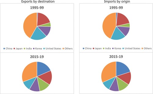
The value of Saudi Arabia’s international trade has increased over time and so has the composition of its trading partners. Trade with developing Asia has been leading the increase. In 2015–2019, China accounted for 18 percent of Saudi Arabia’s total merchandise exports and 20 percent of its imports – in both cases multiple times higher than the shares in 1995–1999. Trade with the United States halved during the same period (Figure 3).

Figure 3. Saudi Arabia: Merchandise Trade, 1995–2019 (Percent of Total). Source: IMF Direction of Trade Statistics.

2.4.2. Financial flows

Assessing the geographical composition of financial flows is complicated by limited data availability. Saudi Arabia does not currently report data to the Bank for International Settlements (BIS) nor participates in the Coordinated Portfolio Investment Survey (CPIS). Nevertheless, recently published data on Saudi Arabia’s International Investment Position indicate that foreign assets amounted to 164.5 percent of GDP in 2020 while external liabilities amounted to 75.6 percent of GDP. Foreign assets include international reserves (64 percent of GDP) – securities, foreign currency, deposits, and gold – and banking sector accounts.

3. Spillover analysis

The sensitivity of the Saudi Arabian economy to developments abroad is examined by evaluating the impact on Saudi variables of shocks to output in its key trading partners as well as a global growth slowdown. Specifically, we study the generalized impulse responses of Saudi GDP, inflation, oil prices and the overall fiscal balance to a one standard deviation negative GDP shock in the United States, China, and the global economy.¹¹ These results provide some intuition on the transmission channels through which foreign GDP shocks affect economic activity in Saudi Arabia. We also study the implications of stress in global financial markets, lower oil prices and a domestic fiscal tightening on the Saudi economy.

3.1. Implications of a slowdown in the United States, China, and the global economy

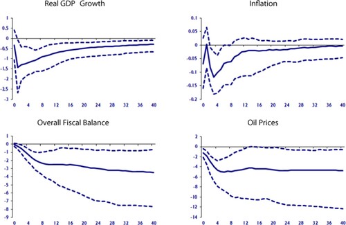
As a result of the dominance of the United States in the global economy, any slowdown there can cause negative spillovers to other economies (including Saudi Arabia), as the recent global financial crisis has shown. Furthermore, the continuing dominance of US debt and equity markets, backed by the still strong global role of the United States dollar, also plays an important role. Cashin et al. (2016) show that countries with substantial trade exposure to the United States economy have a relatively large sensitivity to US economic developments. However, even countries that do not trade as much with the United States are influenced by its dominance through other partners’ trade. Overall, the influence of the United States on other economies remains larger than direct trade ties would suggest, owing to third-market effects together with increased financial integration that tends to foster the international transmission of business cycles. Lower demand for commodities is another channel through which a negative US shock affects countries though its scope is reduced owing to the scaling up of shale oil production (hence the impact on oil prices is not statistically significant, see also Mohaddes & Raissi, 2019). For Saudi Arabia, responsible for about 17 percent of world oil exports, the effect of economic slowdown in the US is particularly large – growth declines by 0.8 percentage points after four quarters (see Figure 4) and we observe a statistically significant decline in Saudi real GDP growth for up to eight quarters. To support growth, a fiscal expansion follows.

Figure 4. Effects of a negative United States GDP shock.

Notes: Figures are median impulse responses to a one standard deviation decrease in the US GDP (equivalent to a temporary growth slowdown of 0.7 percentage points) together with the 5th and 95th percentile error bands. The impact is in percentage points and the horizon is quarterly.

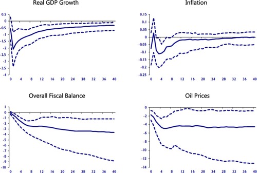
We next investigate the effects of a negative GDP shock in China on the Saudi economy, mainly because China's economy has been rebalancing and its real GDP growth has been slowing down for a few years – from an average of about 10 percent over the period 1980–2013 to 7 percent between 2014 and 2017. In particular, the value of China's imports has been contracting significantly since late 2014, weighing on economic growth in those exporting countries that cater to China's final demand (including Saudi Arabia which is due to expand its market share to China, being the largest importer of oil in the world). This growth slowdown is largely driven by China's gradual ‘rebalancing’ from exports to domestic demand, from manufacturing to services, and from investment to consumption. These developments, together with market concerns about the future performance of the Chinese economy as well as the trade war with the United States, are resulting in spillovers to other economies (especially to commodity exporting countries) through trade links, weaker commodity prices, and financial linkages. Figure 5 shows that the growth slowdown in China (1.5 percentage points) translates into lower overall economic growth for Saudi Arabia, by about 1.2 percentage points after one year (being persistent over the medium term), mainly through its impact on global demand for oil and on associated prices. This finding is to be expected, given the emergence of China as a key driver of the global economy over recent decades (see Fayad et al., 2012 for a similar conclusion). Inflation falls with the growth slowdown and fiscal policy eases to support the economy.

Figure 5. Effects of a negative China GDP shock.

Notes: Figures are median impulse responses to a one standard deviation decrease in the Chinese GDP (equivalent to a temporary growth slowdown of 1.5 percentage points) together with the 5th and 95th percentile error bands. The impact is in percentage points and the horizon is quarterly.

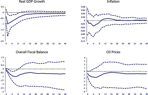
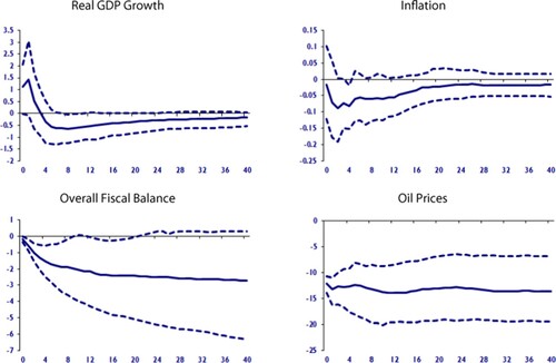
Finally, we examine the implications of a slowdown in the global economy (e.g. from a global trade war) on the economy of Saudi Arabia. Figure 6 shows that one standard deviation decrease in Global GDP (equivalent to a temporary global growth slowdown of 0.8 percentage points) has a significant and long-lasting impact on Saudi Arabia's growth and oil prices. The response appears to be a fiscal expansion in Saudi Arabia to counter the negative growth impact of slower global economic activity and lower oil prices.

Figure 6. Effects of a negative global GDP shock.

Notes: Figures are median impulse responses to a one standard deviation decrease in the Global GDP (equivalent to a temporary global growth slowdown of 0.8 percentage points) together with the 5th and 95th percentile error bands. The impact is in percentage points and the horizon is quarterly.

Overall, the results show that a negative output shock in the United States has a short-lived impact on the Saudi economy, whereas the sensitivity to shocks in China is prolonged. Spillovers vary depending on a host of factors, including the size of bilateral trade flows as well as other real and financial sector linkages present in the data. Moreover, the impact of a one standard deviation real GDP reduction in China is long-lasting, with Saudi real GDP growth falling by more than that in the case of US GDP shock. These results partly reflect the effect that economic developments in each of these countries have on oil prices, with the China shock producing a larger decline in oil prices and adversely affecting the Saudi economy for a longer period. The results also show a strong link between the impact on oil prices and Saudi Arabia's overall fiscal balance (i.e. a deterioration and possibly a fiscal expansion follows to counter the negative growth effects).

3.2. Implications of a potential low oil price environment

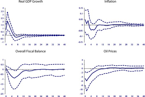
With oil prices down by 40 percent between September and December 2018, the question is whether we have now (again) entered a low oil price environment and whether oil prices will be in the region of $40 and $60 per barrel mainly because of the shale oil and gas revolution in the United States.¹² Clearly, the technological advancements over the last decade have not only reduced the costs associated with the production of unconventional oil, but also made extraction of tight oil resemble a manufacturing process in which one can adjust production in response to price changes with relative ease. This is in stark contrast to other extraction methods (e.g. offshore extraction), which require large upfront spending and involve relatively long lead times, and more importantly, once the process is operational changing the quantity produced can be difficult. Therefore, one of the implications of the recent oil revolution is that US production can play a significant role in balancing global demand and supply, and this in turn implies that the current low oil price environment could be persistent (albeit in a world without wars).

In Figure 7, we show the implications of a new oil order for the Saudi economy. The sharp fall in oil prices initially and maybe surprisingly leads to a boost in economic growth, but this is because of higher social spending of the type seen after the Arab spring and the fall in oil prices in 2014. Moreover, supply-driven lower oil prices could boost economic activity in other economies and in turn dampen the negative growth impact on Saudi Arabia. However, over the medium term, Saudi Arabia experiences a negative growth impact of around 0.5% despite a fiscal expansion of about 2.5% of GDP.

Figure 7. Effects of a negative oil price shock.

Notes: Figures are median impulse responses to a one standard deviation decrease in the oil prices (about 12 percent) together with the 5th and 95th percentile error bands. The impact is in percentage points and the horizon is quarterly.

We expect other major oil exporters in the region to experience similar slowdown in their GDP growth and an increase in fiscal deficits. We also expect negative growth effects (although smaller) for oil-importers in the MENA region with strong economic ties with oil exporters in the region (for instance Jordan and Egypt), through spillover effects. In particular, Mohaddes and Raissi (2019) show that following an expansion in US oil supply and the resulting fall in oil prices, the gains from lower oil prices for most oil-importers in the MENA region, are offset by a decline in external demand/financing by MENA oil-exporters given strong linkages between the two groups through trade, remittances, tourism, foreign direct investment, and grants. They also argue that for several countries in this group, low pass-through from lower global oil prices to domestic fuel prices limits the impact on disposable incomes of consumers and profit-margins of firms, and thereby contains the positive effect on economic growth of lower oil prices in these countries.

3.3. Implications of stress in global financial markets

Stress in global financial markets could emanate from an increase in risk premiums in reaction to a decline in investor sentiment triggered by a deteriorating outlook (including from trade tensions), policy tightening in advanced economies, or weak policy frameworks amidst concerns about debt in some euro area countries. Such shocks could lead to higher interest rates, exchange rate volatility, corrections in stretched asset valuations (for example, equity and real estate), and sudden international financial flow reversals. These developments would strain leveraged companies, households, and sovereigns; worsen bank balance sheets and profitability; and damage the public finances of advanced and emerging market economies. We examine the spillover effects of stress in global financial markets on the Saudi economy next.

While we would have expected that a one standard deviation shock to the financial stress index ($FS{I}_t$) – which is equivalent to about ⅔ of the tightening that happened during the European sovereign debt crisis and ⅒ of the global financial crisis shock – would have an adverse impact on economic activity in commodity exporters through the commodity-price channel (indeed we observe a short-term fall in oil prices), for Saudi Arabia this is not the case (Figure 8). This is because following stress in global financial markets, the Saudi fiscal authorities stimulate demand, leading to an increase in economic growth for a few quarters, but no significant effects in the medium term.

Figure 8. Effects of stress in global financial markets.

Notes: Figures are median impulse responses to a one standard deviation increase in FSI (about ⅔ of the tightening that happened during the European sovereign debt crisis and ⅒ of the global financial crisis shock) together with the 5th and 95th percentile error bands. The impact is in percentage points and the horizon is quarterly.

3.4. Implications of domestic fiscal policy adjustments

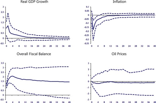
In Figure 9, we look at the implications of fiscal policy adjustment in Saudi Arabia (a one standard deviation increase in Saudi Arabian overall fiscal balance) and its implications for domestic economic growth. Specifically, we study the average macroeconomic effects of changes in the overall fiscal balance in Saudi Arabia. However, these average effects mask the heterogenous multiplier effects of different fiscal instruments (tax and spending measures) – see Ramey (2019) for a survey. While we would have expected a fiscal tightening to cause a temporarily fall in economic growth in Saudi Arabia, this is not borne by the data as the estimated impact on economic growth is not statistically significant (except for the first quarter for which it is positive and significant). We conjuncture that cutting subsidies and handouts may not necessarily have a significant impact on economic growth, since a significant share of these expenditures is poorly targeted. Moreover, the impact is not necessarily linear (could be negative in response to a large-enough spending cut) and also depends upon the quality of adjustment (how growth-friendly they are). If domestic fiscal adjustment reduces distortions in the economy and is complemented with structural reforms, it could in fact boost growth. The impact on oil prices is also not statistically significant considering the determination of oil prices in global markets.

Figure 9. Effects of an increase in Saudi overall fiscal balance.

Notes: Figures are median impulse responses to a one standard deviation increase in Saudi Arabian overall fiscal balance together with the 5th and 95th percentile error bands. The impact is in percentage points and the horizon is quarterly.

4. Conclusions

We developed a quarterly macro-econometric model for the Saudi economy and integrated it within a compact model of the world economy (including the global oil market). Estimating a Global VAR (GVAR) model for 33 countries over the period 1981Q1–2018Q2, we analyzed the macroeconomic implications of shocks on the Saudi economy. Our modelling approach allowed us to disentangle the size and speed of the transmission of growth shocks originating from China, the United States, and the global economy to Saudi Arabia, as well as to study the implications of stress in global financial markets, a potential low oil price environment and a domestic fiscal policy tightening on the Saudi economy.

Our results showed that Saudi Arabia's economy is becoming more sensitive to developments in China than to shocks in the United States – in line with the direction of evolving trade patterns and China's growing role in the global oil market. A global growth slowdown (e.g. from a global trade war) could have significant implications for Saudi Arabia and the oil market. We also observed that a potential low oil price environment and tighter global financial conditions could both have a significant negative effect on the Saudi economy. The negative growth impact is mitigated by domestic fiscal expansions. Finally, a domestic fiscal adjustment in Saudi Arabia were found not to have a statistically significant effect on economic growth. We argue that the sign of the impact would depend upon the size of fiscal adjustment, the quality of tax and spending measures adopted, and whether they are complemented with structural reforms or not. Overall, we have shown that developments abroad have substantial implications for economic activity in Saudi Arabia.

Acknowledgments

The views expressed in this paper are those of the authors and do not necessarily represent those of the United Nations Economic and Social Commission for Western Asia (UN ESCWA), the International Monetary Fund (IMF) or its policy. We are grateful to Raimundo Soto (the Editor) and an anonymous referee for helpful suggestions.

Disclosure statement

No potential conflict of interest was reported by the authors.

Notes

1 Since May 1981, the Gulf Cooperation Council (GCC) countries, constituting of Bahrain, Kuwait, Qatar, Oman, Saudi Arabia, and the United Arab Emirates, have developed strong political and economic alliances.

2 Our sample of 1981Q2–2018Q2 excludes the structural breaks arising from the Covid-19 pandemic and the war in Ukraine. For a GVAR analysis of Covid-19 implications, see Chudik et al. (2021a).

3 See Chudik et al. (2021b) for a study on the effectiveness of global fiscal support in response to Covid-19.

4 See: https://vision2030.gov.sa/en

5 The GCC countries peg their exchange rate against the US dollar since 2003. The current exchange rates are fixed for all the six GCC countries, except Kuwait that pegs its currency against a basket of currencies since 2007.

6 Dees et al. (2007) derive the GVAR as an approximation to a global unobserved common factor model, and show that it is quite effective in dealing with the common factor interdependencies and international co-movements of business cycles.

7 To the extent that unobserved common shocks affect any of the variables in the GVAR model (e.g. uncertainty factor or risk shocks may manifest themselves in equity price movements, fluctuations in exchange rates, spreads, and commodity prices, among others), country-specific foreign variables act as proxies for those latent factors. This is also confirmed by Monte Carlo experiments reported in Kapetanios and Pesaran (2007), where they show that the estimators that make use of cross-section averages (star variables in the context of VARX*) out-perform other estimators based on principal components.

8 The main justification for using bilateral trade weights, as opposed to financial weights, is that the former has been shown to be the most important determinant of national business cycle co-movements (see Baxter & Kouparitsas, 2005).

9 Weak exogeneity test results for all countries and variables are available upon request.

10 See also Cashin et al. (2017a), Mohaddes and Pesaran (2016), and Mohaddes and Pesaran (2016, 2017) for a similar approach.

11 A one standard deviation shock to economic activity in the United States, China and the world is equivalent to a growth slowdown of 0.7, 1.5, and 0.8 percentage points, respectively.

12 Oil prices have increased significantly since 2021Q2 with the rebound in economic activity after easing of Covid-19 restrictions and the accompanying large fiscal support as well as the recent war in Ukraine.

References

- Baxter, M., & Kouparitsas, M. A. (2005). Determinants of business cycle co-movement: A robust analysis. Journal of Monetary Economics, 52(1), 113–157. https://doi.org/10.1016/j.jmoneco.2004.08.002
- Bhanumurthy, N. and N. Sarangi (2019). A fiscal-monetary interaction model for inclusive growth in the middle-income Arab countries: Application to Egypt’s economy. ESCWA Working Paper (forthcoming).
- Cardarelli, R., S. Elekdag, and S. Lall (2009). Financial stress, downturns, and recoveries. IMF Working Paper WP/09/100.
- Cashin, P., Mohaddes, K., & Raissi, M. (2016). The global impact of the systemic economies and MENA business cycles. In I. A. Elbadawi & H. Selim (Eds.), Understanding and avoiding the oil curse in resource-rich Arab economies (pp. 16–43). Cambridge University Press.
- Cashin, P., Mohaddes, K., & Raissi, M. (2017a). Fair weather or foul? The macroeconomic effects of El Nino. Journal of International Economics, 106, 37–54. https://doi.org/10.1016/j.jinteco.2017.01.010
- Cashin, P., Mohaddes, K., & Raissi, M. (2017b). China's slowdown and global financial market volatility: Is world growth losing out? Emerging Markets Review, 31, 164–175. https://doi.org/10.1016/j.ememar.2017.05.001
- Cashin, P., Mohaddes, K., Raissi, M., & Raissi, M. (2014). The differential effects of oil demand and supply shocks on the global economy. Energy Economics, 44, 113–134. https://doi.org/10.1016/j.eneco.2014.03.014
- Chudik, A., Mohaddes, K., Pesaran, M. H., Raissi, M., & Rebucci, A. (2021a). A counterfactual economic analysis of COVID-19 using a threshold augmented multi-country model. Journal of International Money and Finance, 119, 102477. /1–26. https://doi.org/10.1016/j.jimonfin.2021.102477
- Chudik, A., Mohaddes, K., & Raissi, M. (2021b). COVID-19 fiscal support and its effectiveness. Economics Letters, 205, 109939. /1–5. https://doi.org/10.1016/j.econlet.2021.109939
- Chudik, A., & Pesaran, M. H. (2013). Econometric analysis of high dimensional VARs featuring a dominant unit. Econometric Reviews, 32(5-6), 592–649. https://doi.org/10.1080/07474938.2012.740374
- Chudik, A., & Pesaran, M. H. (2016). Theory and practice of GVAR modeling. Journal of Economic Surveys, 30(1), 165–197. https://doi.org/10.1111/joes.12095
- Dees, S., di Mauro, F., Pesaran, M. H., & Smith, L. V. (2007). Exploring the international linkages of the Euro Area: A global VAR analysis. Journal of Applied Econometrics, 22(1), 1–38. https://doi.org/10.1002/jae.932
- Dees, S., Hashem Pesaran, M., Vanessa Smith, L., & Smith, R. P. (2014). Constructing multi-country rational expectations models. Oxford Bulletin of Economics and Statistics, 76(6), 812–840. https://doi.org/10.1111/obes.12046
- Elbadawi, I., & Soto, R. (2011). Fiscal regimes in and outside the MENA region. Working Paper, 654. Giza: Economic Research Forum.
- Fayad G., Raissi M., and T. Rasmussen (2012). “Global interconnectedness: Economic spillovers to and from Saudi Arabia”, Saudi Arabia: Selected issues (IMF Country Report No. 12/272). International Monetary Fund.
- Kapetanios, G., & Pesaran, M. H. (2007). Alternative approaches to estimation and inference in large multifactor panels: Small sample results with an application to modelling of asset returns. In G. Phillips & E. Tzavalis (Eds.), The refinement of econometric estimation and test procedures: Finite sample and asymptotic analysis (pp. 239–281). Cambridge University Press.
- Lee, K., & Pesaran, M. H. (1993). Persistence profiles and business cycle fluctuations in a disaggregated model of UK output growth. Ricerche Economiche, 47(3), 293–322. https://doi.org/10.1016/0035-5054(93)90032-X
- MacKinnon, J. G. (1991). Critical values for cointegration tests. In R. Engle & C. Granger (Eds.), Long-run economic relationships: Readings in cointegration, chapter 13 (pp. 267–276). Oxford University Press.
- Mohaddes, K., & Pesaran, M. H. (2016). Country-specific oil supply shocks and the global economy: A counterfactual analysis. Energy Economics, 59, 382–399. https://doi.org/10.1016/j.eneco.2016.08.007
- Mohaddes, K., & Pesaran, M. H. (2017). Oil prices and the global economy: Is it different this time around? Energy Economics, 65, 315–325. https://doi.org/10.1016/j.eneco.2017.05.011
- Mohaddes, K., & Raissi, M. (2018). Compilation, revision and updating of the global VAR (GVAR) database, 1979Q2-2016Q4. University of Cambridge: Faculty of Economics (mimeo).
- Mohaddes, K., & Raissi, M. (2019). The U.S. oil supply revolution and the global economy. Empirical Economics, 57(5), 1515–1546. https://doi.org/10.1007/s00181-018-1505-9
- Nabli, M., J. Keller, and M. Veganzones. (n.d.). Exchange rate management within the Middle East and North Africa region: The cost to manufacturing competitiveness (Mimeo).
- Pesaran, M. H., Schuermann, T., & Weiner, S. (2004). Modelling regional interdependencies using a global error-correcting macroeconometric model. Journal of Business & Economic Statistics, 22(2), 129–162. https://doi.org/10.1198/073500104000000019
- Pesaran, M. H., & Shin, Y. (1996). Cointegration and speed of convergence to equilibrium. Journal of Econometrics, 71(1-2), 117–143. https://doi.org/10.1016/0304-4076(94)01697-6
- Pesaran, M. H., Shin, Y., & Smith, R. J. (2000). Structural analysis of vector error correction models with exogenous I(1) variables. Journal of Econometrics, 97(2), 293–343. https://doi.org/10.1016/S0304-4076(99)00073-1
- Ramey, V. A. (2019). Ten years after the financial crisis: What have we learned from the renaissance in fiscal research? Journal of Economic Perspectives, 33(2), 89–114. https://doi.org/10.1257/jep.33.2.89
- United Nations. (2019). Financing for sustainable development report 2019. New York.
- United Nations Economic and Social Commission for Western Asia. (2017). Rethinking fiscal policy for the Arab region. E/ESCWA/EDID/2017/4. Beirut.
- World Bank. (2019). Gulf economic monitor: Issue 4/May 2019. World Bank Group.