Linear and non-linear regression model fitting of testicular three-dimensional growth in Miranda donkeys

Abstract

In endangered donkey populations, reproductive performance is one the most important areas to study, provided its connection with conservation opportunities. Among reproductive traits, testicular dimensions, their relationship with body weight and seminal qualitative and quantitative parameters is particularly notable. The aim of the present study was to model the evolution of body weight, testicular length, width and height, volume and gonadosomatic index in Miranda donkeys using in vivo ultrasonography. Data on the aforementioned variables of 23 Miranda donkeys, from 4 to 259 months of age, were fitted to eleven linear and nonlinear models. Cubic function modelling reported the best-fitting properties for almost all variables, except for body weight (sigmoid curve model). Cubic model presented a higher ability to capture interindividual variability (Adj. R² from 0.795 to 0.922) for testicular height, width, length and volume measurements than the rest of fucntions tested. Bayesian information criterion (BIC) values suggest in vivo ultrasonography may be a rather efficient and accurate tool when predicting for the evolution of testicular volume or gonadosomatic index than three-dimensional testicular measurements.

Highlights

• Cubic functions efficiently model testicular dimensions, volume and composite indices evolution.

• Ultrasonography objectively, accurately and reproducibly determines testicular volume.

• Testicular asymmetry physiologically occurs to balance bilateral testicular activity.

Keywords:

• Donkeys
• akaike information criterion
• body weight
• testicular dimensions predictive models
• bayesian information criterion

Introduction

In endangered donkey populations, reproductive performance is one the most important areas to study, provided its connection with the increase in the opportunities for population conservation (Navas et al. 2017,2019). Knowledge of testicular morphometric features given its relationship with seminal parameters may provide valuable information not only about the physiological and pathological status of the animals with potentialities for clinical diagnosis, but also for the selection of donkeys to maximise breeding and sperm production opportunities (Quartuccio et al. 2011; Aissanou and Ayad 2020). This achieves a specially great relevance provided the generalised high endangerment status which donkey breeds face, linked to increased inbreeding and reduced genetic diversity levels (Kugler et al. 2008).

Testicular biometry has been suggested to be an indicator of reproductive status and its characterisation has already been documented in donkeys (Ayad et al. 2019; Aissanou and Ayad 2020). Not only the relationship between reproductive status and age has been approached, but also modelling quantitative methods to determine the evolution of testicular structure and function under various physiological and pathological conditions has attracted the attention of researchers (Omar et al. 2013; Aissanou and Ayad 2020). The knowledge of donkeys’ reproductive function through the evaluation of testicular biometry, given its implication in the understanding of donkey reproductive physiology can help to model, explain and predict the breeding potential of individuals. The first steps towards the exploration of testicular biometric parameters and the conditioning factors involved in the variation across individuals was performed recently (Aissanou and Ayad 2020). However, there is limited information on testicular morphometric characteristic of specific donkey breeds, which could presumably be diverse, considering the wide zoometric range that is present from Miniature Mediterranean donkeys to Mammoth Jackstocks (Navas et al. 2016).

Testicular traits such as testicular diameter, testicular length, scrotal circumference, and scrotal length have been used as indirect selection criteria to improve fertility provided their correlations with seminal parameters (Öztürk et al. 1996; Quartuccio et al. 2011). These correlations enable the indirect determination of seminal parameters through the evaluation of testicular morphometry related traits which can be easily measured. Additionally, testicular traits, such as scrotal size and dimension have been reported to be genetically correlated with ovulation rate of females in other species, hence, these may act as indirect determinants of the moment to breed reproductive pairs, seeking the maximisation of chances to obtain successful pregnancies (Bilgin et al. 2004).

Although the modelling of testicular morphometric traits using linear and nonlinear regression models have been frequently approached in literature for other species (Bilgin et al. 2004; Loaiza-Echeverri et al. 2013; Karakuş et al. 2020), for equids and particularly for donkeys, the information present in literature is still scarce and normally just based on stating the relationship between body weight or testicular growth along and age at specific time points (Onoda et al. 2011; Aissanou and Ayad 2020). Still, no detailed study has been performed in regards the use of linear and non-linear models to determine the development of testicular traits up to the present date, in the donkey species, to the best of authors’ knowledge.

The present study was developed in the context of a major project aiming at determining the relationship between body weight, testicular development and combined indices and seminal parameters and their evolution in time. The evaluation of the relationship between body weight, testicular development and combined indices and seminal parameters was dealt with in the previous publication by Martins-Bessa et al. (2021). The aims of this work were to determine the fitness properties of linear and non-linear models for describing body weight evolution, growth of testicular traits and of their combined indices in Miranda donkeys in order to be able to issue modelling equations that can be used to predict for testicular functional outcomes, which can become an invaluable tool to assist in the reproductive management and as a result, in the conservation programs of these precious animal genetic resources.

Material and methods

Study sample

Study sample comprised 23 clinically healthy Miranda donkeys, with ages ranging from 7 to 259 months and a body weight that ranged from 120 to 400 Kg (juvenile donkey foals average 11.1 ± 2.77 months old and 160.3 ± 24.7 Kg; mature jacks average of 79.9 ± 50.3 months old and 279.5 ± 54.4 Kg, respectively) (Figure 1). The body condition (BCS) was 5 ± 0.5 (scored 1–9). The donkeys comprising the study sample were housed at the Veterinary Teaching Hospital of UTAD (VTH-UTAD, Vila Real, Portugal). Formal consent and collaboration of Association for Study and Protection of the Donkey Breed Burro de Miranda (AEPGA) was received. The study was carried out under the framework of a scientific agreement of cooperation signed between both institutions. Clinical procedures were conducted following national laws for animal welfare and experimentation as with the European Directive 2010/63/EU for animal experiments and the Directive Hospital Committee (Approval Ref. 408/VTH-UTAD). General (Clinical, BCS and weight) and testicular exams were performed during spring-summer season.

Figure 1. Sample distribution. P25: value at 25% of observations; P50: value at 50% of observations and P75: value at 75% of observations.

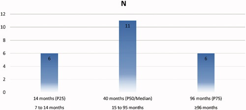
Clinical and genital examinations were performed previous to ultrasonographic (US) examination. Body weight (BW) (Kg) was recorded using an equine digital floor weighting scale (Salter Brecknell^® PS-3000HD Floor – Veterinary Scale, USA). Animals were allocated to two groups by age; juvenile to prepubertal (n = 6) (≤14 months) and mature (n = 17) (≥24 months). In order for animals to be considered for this study, both of their testicles must be at scrotal position, symmetrical, of normal size in relation to age, normal consistency and without echogenic changes in the testicular parenchyma, epididymis and spermatic cord.

Testicular morphometry evaluation

Ultrasonography examination of testicular measurements were performed using a Philips^® CX30 Portable Ultrasound (Philips^®, Amsterdam, Holland) with a sectorial 3.0–7.0 MHz transducer, following the premises developed by Love (2014). Longitudinal and transversal plans were performed on each testicle, excluding epididymis measurements. Three scan rounds were performed placing electronic cursors at the limit of tunica albuginea. Right and left testicle length (L), height (H) and width (W) (cm) were computed. Right and left testicular volumes (TV) were then calculated using the Lambert formula, TV = L × W × H × 0.5233 (Love 2014). Total testicular volume (TTV) or the sum of the right and left TV was also individually calculated. In the calculation of the gonadosomatic ratio (GSI) (%), i.e. testicular weight/BW, the TTV (cm³) was transformed into grams, considering testicular density in mammals is very close to one (Johnson and Neaves 1981). Testicular morphometry and volumetric evaluation were performed from 09 November 2017 to 24 July 2019. A total of 31 measurements were taken.

Statistical analyses

Parametric assumptions testing

Two approaches were followed in order to fit the requirements of normality test to report valid conclusions. On the one hand, Shapiro-Francia W’ test (Stata Version 15.0 software) was used to evaluate the normality assumption (for 50 < n < 2500 samples) in the morphometry dataset (Supplementary Table S1).

Autocorrelation analysis was performed by testing the Durbin-Watson method (Durbin 1970) using the Linear regression test of regression procedure in SPSS version 25.0. The Durbin-Watson (DW) test is reliable for sample sizes larger than 15 (Greenberg et al. 2020) and the statistic that it reports ranges from 0 to 4 can only be used to test for autocorrelation in ordered time or spatial series (Chen 2016) such as the evolution of testicular morphometry in time. When DW statistic is below the critical value of 2, evidences of positive autocorrelation are suggested. DW values over this upper critical value suggest a lack of statistical evidence about the existence of positive autocorrelation. Contrastingly, if DW is in between the lower and upper critical values, the test is inconclusive (Gujarati and Porter 2003).

Additionally, when performing ordinary least squares regression, the variance of the residuals must be homogeneous across levels of the predicted values (homoscedastic). Residual values derive from the difference between observed and predicted values. Well-fitted models do not describe variable patterns when the residuals plotted against the fitted values. If the variance of the residuals is non-constant then the residual variance is said to be heteroscedastic. Durbin Watson and Scatter plots were performed using SPSS Statistics for Windows statistical program, Version 25.0.

Model choice decision rationale

Nonlinear models have been widely contrasted as suitable methods to fit for testicular growth in several local breeds belonging to a wide spectrum of species (Bilgin et al. 2004; Loaiza-Echeverri et al. 2013) which include equids (Silva et al. 2021). However, other alternatives, such as mixed models with random and fixed effects, have been formerly suggested in literature to fit for the same aim, furthermore when additional factors are to be considered while modelling (Cole et al. 2014). Mixed models (random and fixed) have several desirable properties, but their use needs is compelled to certain assumptions being met (El Halimi 2005).

As suggested by Harrison et al. (2018), mixed models, either it is using fixed or random effects, need at least five ‘levels’ (groups) for a random intercept term to achieve robust estimates of variance. This was also supported by Gelman and Hill (2007) and Harrison (2015), who suggested the fact that fixed or random effects, with lower than 5 levels may not accurately estimate between population variance, due to variance estimate collapsing to zero, which in turn makes the model equivalent to nonlinear modelling (Gelman and Hill 2007) or be non-zero, but incorrect when the small number of levels (groups) from which samples were taken is not representative of true distribution of means. This was also addressed to be a potential source for variance and covariance distortion as a direct consequence of too few levels of a fixed or random effect as suggested by Silk et al. (Silk et al. 2020).

Furthermore, fixed and random effects are generally inconsistent in nonlinear model as n grows (Newey 2007). This rationale may make compulsory to apply integration methods such as adaptive Gaussian Quadrature method to prevent distortion from occurring (Afrouziyeh et al. 2021), which in turn increases the complexity of the methods used.

In our study, including the animal as a random effect may have accounted for 23 levels, strongly preventing against the use of non-linear mixed (random) models due to the aforementioned reasons. Furthermore, as the same animals were repeatedly measured along the course of the study, those random effects corresponding to the same animal are correlated, hence, this acts against the assumption of independence of observations being met (Chan and Kuk 1997). Failing to meet the assumption of non-independence may eventually lead to pseudoreplication and inflated Type I error rates. As a result, given animals were measured repeatedly, we decided to run nonlinear procedures.

The different models used comprised a variable number of curve shape parameters, thus they differed in terms of model complexity. The number of parameters considered in a model and the nature of its mathematical function may indeed be responsible for the better fitting properties of certain models against others as suggested by Pizarro et al. (2020a, 2020b).

In this context, as suggested by Curran et al. (2010), there are few strict requirements for the types of data that can be modelized using growth models, but still these must be considered. First, an adequate sample size is needed to reliably estimate growth models. However, sample size adequacy strictly depends in part on the characteristics of the research design, for instance, growth model complexity, amount of variance explained by the model, among others. In these regards, although growth models have successfully been fitted to samples as small as n = 22 in unrelated fields (Huttenlocher et al. 1991), the lowest sample size limit for testicular growth modelling is around 30 individuals (given the complexity that sampling involves which is specially hindering in endangered species) (Karakuş et al. 2010) and preferable sample sizes often approach at least 100 individuals.

Furthermore, the close relationship between the number of sampled individual and the number of repeated observations per individual, may be more crucial for model estimation and statistical power when growth models are used to fit for longitudinal data than when other computationally and paramterically simpler nonlinear models are used (Muthén and Curran 1997a, 1997b; Serroyen et al. 2009).

Contextually, as suggested by literature (Curran et al. 2010), although certain freedoms may be allowed (when the modellization of partially missing data is aimed), growth models typically require at least three repeated measures per individual for at least a sizeable portion of the cases. The reason for this relies in the fact that three repeated measures permit to trace a linear trajectory, hence, there is more observed information than estimated information.

Additionally, maximum likelihood estimation method assumes that the repeated measures are continuous and normally distributed. However, other nonlinear methods of estimation allow for measures that are continuous and non-normally distributed (Satorra 1990), such as those in our study and which are common to sampling from endangered species, or even discretely or ordinally scaled (Mehta et al. 2004). Consequently, even if growth models may be fitted, care must be taken to maximally correspond to the characteristics of the given data set.

Statistical considerations before regression

The presence of outliers reduces predictive power and promotes the violation of the assumption of normally distributed data. Outliers in our data sample were detected using the identify outliers procedure of the Analyze/Built-in analysis of the column analyses package of GraphPad Prism version 8.3.0. To prevent the influence by outliers, the ROUT method was used. ROUT method combines Robust regression and Outlier removal and bases on the False Discovery Rate (FDR). A maximum desired FDR must be predefined (Q coefficient). ROUT method assumes data to be sampled from a Gaussian distribution with the exception of any outliers. When this assumption is violated, outliers may follow the same distribution as data.

The value of coefficient Q determines the strength of the ROUT method to detect outliers. The higher the value of Q, the less strict the threshold for detecting outliers is, hence, the higher the power to detect outliers will be, but also the more likely it will be for the method to falsely detect them. Setting lower values of Q renders thresholds for defining outliers stricter, hence the power to detect real outliers will be lower but also the chance for falsely considering an observation to be an outlier. A Q coefficient of 1% is recommended as a default (Motulsky and Brown 2006), which may determine a false discovery rate for detecting outliers of less than 1%.

Model functions and curve shape parameters

One linear model and ten non-linear models were used to describe the evolution of ultrasound testicular measurements of the 23 donkeys in the study sample. The functions for each of the models fitted, the letters used to identify them across this manuscript and the model syntax to be copied and pasted in the non-linear regression task from the Regression procedure of SPSS version 25.0 (IBM Corp. 2017) are presented in Table 1.

Table 1. Models and model syntax.

Model	Initials	Model syntax/equation
Linear	LIN	Y = b0 + (b1 * t)
Logarithmic	LOG	Y = b0 + (b1 * ln(t)
Inverse	INV	Y = b0 + (b1 / t)
Quadratic	QUA	Y = b0 + (b1 * t) + (b2 * t**2)
Cubic	CUB	Y = b0 + (b1 * t) + (b2 * t**2) + (b3 * t**3)
Power	POW	Y = b0 * (t**b1) or ln(Y) = ln(b0) + (b1 * ln(t))
Compound	COM	Y = b0 * (b1**t) or ln(Y) = ln(b0) + (ln(b1) * t)
S-curve	SCRV	Y = e**(b0 + (b1/t)) or ln(Y) = b0 + (b1/t)
Logistic	LGI	Y = 1 / (1/u + (b0 * (b1**t))) or ln(1/y-1/u) = ln (b0) + (ln(b1) * t)
Growth	GRO	Y = e**(b0 + (b1 * t)) or ln(Y) = b0 + (b1 * t)
Exponential	EXP	Y = b0 * (e**(b1 * t)) or ln(Y) = ln(b0) + (b1 * t)

t represents time expressed in month units. Accessed from IBM Corp (2015)

The curve estimation task from the Regression procedure of SPSS version 25.0 (IBM Corp. 2017) using the Levenberg-Marquardt method of iteration was used to iteratively determine each parameter of the curve (Intercept, a, b, c, and d). The iterative process considered as many rounds as it was necessary until a tolerance convergence criterion of 10⁻⁸ was reached as suggested by other authors (Dematawewa et al. 2007), provided stricter criteria have reported the same outcomes out of a slightly higher number of iterations (Feistauer et al. 2004; Arora 2017). After convergence was reached, initial parameters were predefined to implement model fitting procedures.

Model selection criteria

The selection criteria used to determine the best explicative and predictive models included Residual Sum of Squares (RSS), Mean Squared Prediction Error (MSPE), Adjusted R Squared (Adj. R²) and its standard deviation across does, Akaike (AIC), corrected Akaike (AICc), and Bayesian information criteria (BIC). RSS computes the explanatory ability of the model. Cross-validated Minimum Mean-Square Residual or error (MMSE) (Asherson et al. 2008), was chosen to determine error variation as an alternative to cross-validated Mean Squared Error (MSE) which has been suggested to be influenced by the number of parameters (Val-Arreola et al. 2004) if sample sizes are limited.

Curve shape parameters computation for the best fitting model

Computational methods used to determine peak values are reported in Supplementary Table S2. If the computation of a peak was not possible, change in variable units per event was calculated as suggested in Table S2. Symbolab^® Mathematical calculation tool for education (Eqsquest 2020) was used to determine relative maxima (peak) when these could not be found in literature.

K-fold cross-validation

K-fold cross-validation was performed to check for overfitting and out of sample prediction. To this aim, Crossfold module (code: ssc install crossfold) (Daniels 2013) for STATA/MP software v16.0 (StataCorp 2019) was used to perform K-fold cross-validation on best performing models to evaluate their ability to fit out-of-sample data. The K-fold cross-validation was chosen as it has been reported to be more suitable than other methods such as Monte Carlo cross-validation when testing small data sets (Sall et al. 2017). K-fold cross-validation splits the data randomly into k partitions, then fits the specified model using the other k-1 groups for each partition and uses the resulting parameters to predict the dependent variable in the unused group. According to Fushiki (2011), although K-fold cross-validation may be preferred from a computational standpoint, its upward bias may trouble accuracy determination in real data analysis when K is small (Brunori et al. 2019). Consequently, large K folds are recommended when sample is lower than 1000 data points. As a 10-fold validation was chosen, data was split into 10 groups and for each group we fit the final specification using the other K-1 groups. The resulting parameters were used afterwards to predict the dependent variable in the unused group. We compare average root mean squared errors and adjusted determinant coefficients from 10 regressions with coefficients from beta model on observed data.

Results

Summary of the results for each model explicative and predictive power via the evaluation of fitting and flexibility criteria can be consulted in Tables 2 and 3, respectively.

Table 2. Summary of the results for determination coefficients, curve shape parameters, and peak for best fitting models for all the variables in the study.

Variable	Units	Model	R Square	F	df1	df2	Sig.	Intercept	a	b	c	R/Peak
Body Weight	Kg	S Curve	0.862	1340.95	1	215	0.000	5.707	–6.21			0.8250
Left Testicle Length	cm	Cubic	0.871	478.08	3	213	0.000	1.353	0.20	–0.001	0.000	9.4211
Right Testicle Length	cm	Cubic	0.922	838.74	3	213	0.000	1.261	0.20	–0.001	0.000	9.9544
Left Testicle Height	cm	Cubic	0.883	534.21	3	213	0.000	0.744	0.12	–0.001	0.000	5.9164
Right Testicle Height	cm	Cubic	0.825	333.91	3	213	0.000	1.034	0.09	–0.001	0.000	5.4259
Left Testicle Width	cm	Cubic	0.901	647.43	3	213	0.000	0.771	0.16	–0.001	0.000	6.9044
Right Testicle Width	cm	Cubic	0.894	600.67	3	213	0.000	0.741	0.17	–0.001	0.000	7.5141
Left Testicle Volume	cm^3	Cubic	0.817	307.153	3	206	0.00	–29.673	4.394	–0.026	0.000	192.6565
Right Testicle Volume	cm^3	Cubic	0.833	341.326	3.000	206.000	0.000	–24.232	3.761	–0.021	0.000	169.5926
Total Testicle Volume	cm^3	Cubic	0.830	334.944	3.000	206.000	0.000	–53.956	8.156	–0.047	0.000	362.2239
GSI	cm^3/Kg	Cubic	0.795	265.435	3.000	206.000	0.000	–0.160	0.031	0.000	0.000	1.3963

GSI- gonadosomatic index

Table 3. Summary of the measures for model fitness and flexibility criteria of the best fitting linear or nonlinear regression models for each particular trait.

Traits	SS	df	MS	F	Sig.	RSS	MSPE	MMSE	AIC	AICc	BIC
Body Weight in Kg	33.49	1.00	33.49	1340.95	0.00	5.37	0.03	0.00	–800.70	–800.70	–174180.10
Left Testicle Length in cm	1591.74	3.00	530.58	478.08	0.00	236.39	1.11	0.02	20.57	20.57	4035.32
Right Testicle Length in cm	1653.86	3.00	551.29	838.74	0.00	140.00	0.66	0.00	–93.10	–93.10	–20631.61
Left Testicle Height in cm	624.08	3.00	208.03	534.21	0.00	82.95	0.39	0.00	–206.69	–206.69	–45281.04
Right Testicle Height in cm	503.77	3.00	167.92	333.91	0.00	107.12	0.50	0.00	–151.19	–151.19	–33237.87
Left Testicle Width in cm	1022.12	3.00	340.71	647.43	0.00	112.09	0.53	0.00	–141.35	–141.35	–31101.39
Right Testicle Width in cm	978.36	3.00	326.12	600.67	0.00	115.64	0.54	0.00	–134.58	–134.58	–29631.53
Left Testicle Volume in cm^3	1020889.37	3.00	340296.46	307.15	0.00	228228.37	1107.91	0.00	1470.11	1470.11	308308.20
Right Testicle Volume in cm^3	819385.23	3.00	273128.41	341.33	0.00	164840.68	800.20	0.00	1362.00	1362.00	276086.19
Total Testicle Volume in cm^3	3661822.61	3.00	1220607.54	334.94	0.00	750708.15	3644.21	0.00	1669.76	1669.76	338560.58
Ratio Testicular Volume/Body Weight in cm^3/Kg	37.31	3.00	12.44	265.44	0.00	9.65	0.05	0.00	–673.44	–673.44	–146565.19

Table 4. Mean and Standard Deviation for Testicular biometric parameters in juvenile foal and mature Miranda donkeys.

Testicular biometric parameters	Juvenile		Mature
	Mean	Std. Deviation	Mean	Std. Deviation
Left testicle length (cm)	2.78	0.76	8.08	1.12
Right testicle length (cm)	2.76	0.62	8.00	1.28
Left testicle height (cm)	1.71	0.54	4.80	1.01
Right testicle height (cm)	1.71	0.49	4.47	0.72
Left testicle width (cm)	2.03	0.68	6.07	1.14
Right testicle width (cm)	2.10	0.58	6.05	1.25
Left testicle volume (cm^3)	5.92	4.58	132.08	61.16
Right testicle volume (cm^3)	5.89	4.50	120.24	51.88
Total testicular volume (cm^3)	11.75	8.92	252.32	111.50
GSI	0.08	0.05	0.89	0.33

Approach determination: pre-evaluation of parametric assumptions and descriptive statistics

Supplementary Table S2 suggest all variables resulted to be non-normally distributed and residuals heteroscedastic (p < .01). Consequently, fitting nonlinear regression models and Bayesian inference statistics to compare their outputs may be the most appropriate approach to follow. Supplementary Table S1 presents the descriptive statistics for ultrasonographic (US) testicular measurements.

Considerations prior to regression analyses

One likely outlier was detected and hence was removed from the analyses for left testicular volume, right testicular volume and total testicular volume measured with ultrasonography. The occurrence of outliers from the rest, may be a result of reduced sample sizes (Fung 1993; Motulsky and Brown 2006) but also may address the high biological variability that can be found in populations for testicular volume (Quartuccio et al. 2011).

General outputs derived from regression analyses

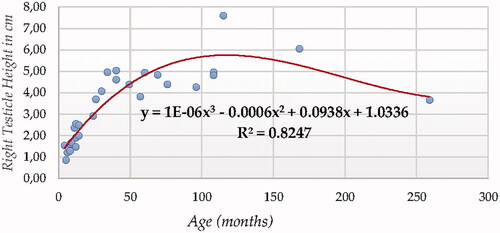
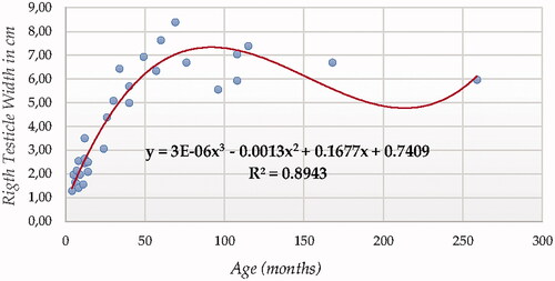
Table 2 shows a summary of the results for determination coefficients, curve shape parameters, and peak for best fitting models for all the variables in the study. Supplementary Table S5 shows the outputs obtained after fitting the eleven models tested in the study. According to best-fitting models body weight change in variable units per time unit is 0.8250 and describes the progressive evolution of body weight with age. For testicular dimension modelling peak in testicle length is 9.4211 cm for left testicle (US) and 9.9544 cm for Right Testicle (US), respectively, with both peaks being attained at around 100 months. For testicle height, peak was 5.9164 cm for Left Testicle (US) and 5.4259 cm for Right Testicle (US), respectively, attained also at around 100 months, though it may postpone 20 months later in right testicle. For testicular width, a peak of 6.9044 cm was reported for Left Testicle (US), while the same peak of 7.5141 cm was reported for Right Testicle (US) at around 100 months. Peak in Left Testicle Volume (US) of 192.6565 cm³ and in Right Testicle Volume (US) of 169.5926 cm³ are attained slightly later (115–120 months), which also occurred for Total Testicle Volume (US) with a peak of 362.2239 cm³. The peak in the ratio between US Testicular Volume and Body Weight of 1.3963 and occurs around, as for other parameters, at 100 months.

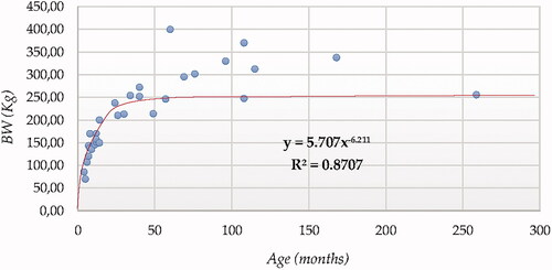
Body weight modelling

For BW, sigmoid curve (SCRV) presented the best fitting properties (Figure 2) as suggested by the higher R squared values followed by the Cubic model (CUB), which was parametrically and computationally more complex.

Figure 2. Body weight (BW) modelling using a sigmoid curve function.

Bilateral testicle length modelling

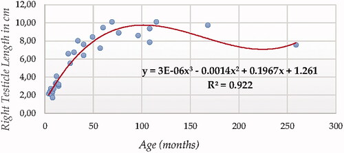
For testicle length (in both testicles using ultrasonography, Figures 3 and 4), Cubic Model (CUB) presented the best fitting properties as suggested by the higher R squared (0.922 and 0.871, for right and left testicle, respectively) values followed by the Quadratic model (QUA), which was parametrically and computationally less complex. The difference in determination coefficient between both testicles was 5.1%.

Figure 3. Left Testicle Length in cm modelling using a cubic function.

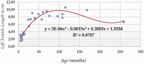
Figure 4. Right Testicle Length in cm modelling using a cubic function.

Bilateral testicle height modelling

For testicle height using ultrasonography (in both testicles, Figures 5 and 6), Cubic Model (CUB) presented the best fitting properties as suggested by the higher R squared values (0.883 and 0.825, for right and left testicle, respectively) followed by the Quadratic (QUA), S Curve (SCRV) and Power (POW) in decreasing order depending on their determination coefficient whose computational complexity in parallel increased. The difference in determination coefficient between two testicles was 5.8%).

Figure 5. Left Testicle Height in cm modelling using a cubic function.

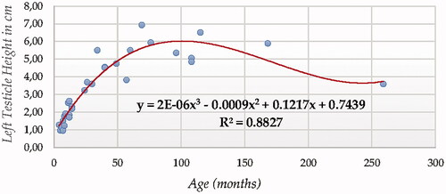
Figure 6. Right Testicle Height in cm modelling using a cubic function.

Bilateral testicle width modelling

For testicle width using ultrasonography (in both testicles, Figures 7 and 8), Cubic Model (CUB) presented the best fitting properties as suggested by the higher R squared values (0.894 and 0.901, for right and left testicle, respectively) followed by the Power (POW), Quadratic (QUA) and S Curve (SCRV) models in decreasing order depending on their determination coefficient whose computational complexity in parallel increased. The difference in determination coefficient between two testicles was 6.9%.

Figure 7. Left Testicle Width in cm modelling using a cubic function.

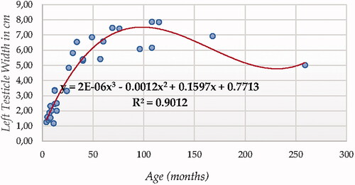
Figure 8. Right Testicle Width in cm modelling using a cubic function.

Bilateral and total testicular volume modelling

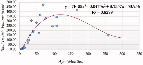
For testicular volume measured using ultrasonography (either individual testicular or total (Figures 9, 10 and 11), Cubic Model (CUB) presented the best fitting properties as suggested by the higher R squared values (0.833 and 0.817, for right and left testicle, and 0.830 for total volume, respectively) followed by the Power (POW), Quadratic (QUA) and S Curve (SCRV) models in decreasing order depending on their determination coefficient whose computational complexity in parallel increased. The difference in determination coefficient between two testicles was 1.6%).

Figure 9. Left Testicle Volume in cm³ modelling using a cubic function.

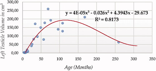
Figure 10. Right Testicle Volume in cm³ modelling using a cubic function.

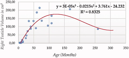
Figure 11. Total Testicle Volume in cm³ modelling using a cubic function.

Bilateral and total testicular volume modelling

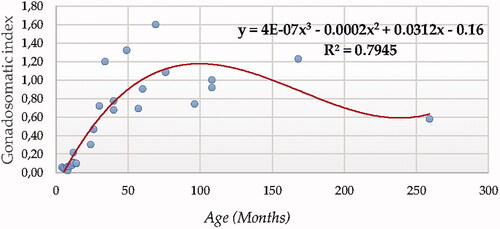
The cubic function reported a determination coefficient for ratio between testicular volume and BW or gonadosomatic index of 0.7945 when ultrasonography was used for testicular measurement (Figure 12).

Figure 12. Gonadosomatic index (GSI) modelling using a cubic function.

Evaluation of model fitness and flexibility criteria

Table 3 shows a summary of the measures for model fitness and flexibility criteria through mean square residual or error and minimum square residual or error (MSE and MMSE), variability explanation power through Akaike Information Criterion (AIC) and Corrected Akaike Information Criterion (AICc) and Predictive power through Bayesian Information Criterion of the best fitting linear or nonlinear regression models for each particular trait.

K-fold cross-validation

As observed in Supplementary Table S5, none of the adjusted determination coefficients nor average root mean standard errors (RootMSE) from 10-fold validation sharply differed from those reported for beta model with observed data. Hence, the model can be accurate enough as to draw valid conclusions from our results.

Discussion

Body weight modelling

The same best fitting properties found in our study for sigmoid curve (SCRV) were also found to best fit for body weight in Thoroughbred horses (Onoda et al. 2011). Thoroughbred horses are seasonal mating animals, raised in northern regions or countries, such as the breed which our study deals with. Foals born yearly in spring generally show a typical seasonal compensatory growth pattern, in which their growth rate declines in the first winter and increases in the next spring. These authors suggested Sigmoid curves adjust for this compensatory growth. Contrastingly, De Palo et al. (2016) reported Martina Franca donkey breed does not describe this compensatory growth, although this physiological response, recorded in many species and breeds (France et al. 1996), which suggests breed dimorphism may occur. In this context, other factors such as the nutrition patterns followed may condition body growth patterns as well, as suggested by De Palo et al. (2016). For instance, these authors suggested growth ratio, live and carcase weight of artificially suckled donkey foals to be higher than naturally suckled donkey foals during the first 6 months of life.

The use of compensatory growth has been used in other species such as bovines seeking the benefit of the owners. For instance, an effective strategy to recover weight loss after work in oxen was to feed them after the working period began as they rapidly regain body weight through compensatory growth (Pearson et al. 1996). Miranda donkeys are predominantly used as draught animals in agriculture and as pack animals in tourism, hence their working qualities may be analogous to those in oxen (Kugler et al. 2008; Delgado et al. 2014). These may explain the lack of occurrence of compensatory growth found in Martina Franca donkey breed, provided their zoometrics more than their traditionally use as draught and pack animals, promoted their application for mule production with Murge-horses, which became relevant both in Italy and internationally (Kugler et al. 2008).

Bilateral testicle dimensions (length, height, width) and volume modelling

Average testicular volume in Miranda juvenile donkey foals measured using ultrasonography was 11.7 ± 8.9 cm³, while for mature donkeys it was 252.3 ± 111.5 cm³ (Table 4). These results contrast those reported by Aissanou and Ayad (2020) for Algerian donkeys and Nordestino Brazilian donkeys (Rocha et al. 2018), smaller sized breeds. Our study comprised both juvenile and mature animals as the aims of this paper made it necessary to determine and modelling the evolution of testicular biometry. These results may suggest age, breed or even methodology used to determine measurements may imply differences in testicular volume being reported. For instance, the values present in mature Miranda donkeys resemble those found in larger breeds such as those studied by Canisso et al. (2009) and Omar et al. (2013) for testicular volume in Pêga and Egyptian breeds. Although Egyptian breeds are rather undefined, with anecdotal occurrence of standardised breeds such as Hassawi (Porter et al. 2016; Shawaf et al. 2017), these have been traditionally connected to breeds of a larger size such as the Andalusian donkey (Navas et al. 2018).

The development of models to predict and describe the evolution of testicle dimensions is scarce as these dimensions have rather been considered the independent variables in models rather than considered the dependence between testicular dimensions evolution and time (Walkden-Brown et al. 1994). In this context, Restricted cubic splines have been frequently used for the modelling of abnormal (tumoral) testicular growth in humans (Vergouwe 2003). However, these authors suggest coding continuous covariables may be an issue to solve in prediction modelling given model flexibility may be too large, leading to a too close fitting of idiosyncrasies in the data set rather than true patterns. Royston (2000) recently proposed to select a parametric function (for instance cubic) by comparison with a cubic smoothing spline as the reference curve. Our results are in agreement with those found by Schoeman and Combrink (1987), who reported cubic polynomials to be the best fitting models to predict for testicular dimensions as a function of age when compared to linear or quadratic functions in one crossbred and two sheep breeds, reporting R² values over 0.7.

Differences in R² may be ascribed to testicle dimensional differences derived from compensatory growth. It seems that as compensatory growth increases, R² values increase too, thus, the model fits better the data as its ability to capture variability improves. In these regards, the differences in determination coefficient ranged from 5 to 7% and favoured length and height in the right testicle while the opposite was described for the width dimension. This may be indicative of an increased differential growth of each testicle. Such testicular asymmetry has been reported to occur in response to changes in the counterpart testicle after castration (Omar et al. 2013). For instance, Omar et al. (2013) reported a similar compensatory effect after in the right testicle occurred the removal of left testis in donkeys. Unilateral orchiectomy has been reported to increase the mean diameter of seminiferous tubules by 21% and of their lumina by 51% (Barnes et al. 1980b). Consequently, our findings may suggest testicular asymmetry may occur physiologically, without the need of a drastic removal or failure of the testicles, although certain circumstances such as unilateral castration and overwork may startle the process as it was also reported in donkeys (Omar et al. 2013) or other species (Cassinello et al. 1998).

A previous work supports this “asymmetric compensation hypothesis” in birds which suggests one of the testis could serve as a ‘back-up’ for any reduced function of the other and provides a mechanism to explain intraspecific variation in degree and direction of gonad asymmetry (Calhim and Birkhead 2009). These authors ascribed this compensation to the increase in serum LH and FSH concentrations and, potentially higher intratesticular testosterone (Hoagland et al. 1986; Hoagland and Bolt 1986).

Testicular dimensions better fit cubic functions rather than quadratic functions. As suggested by Nipken and Wrobel (1997) in bovines, histophysiological features indicative of the spermatogenetic efficiency increase continuously from the age of 1.5 years to the middle of sexual maturity (5–6 years). Afterwards, these features slightly later undergo continuous retrogression, which suggests, the adult testis may be an organ in permanent change.

Our results agree with those reported by Richard et al. (2017), who suggested seasonality of total testicular volume was best described by a cubic fixed effect model in belugas. These results are consistent with observations of reproductive seasonality, and suggest a relatively low demand for sperm in this species. These results are consistent with those reported by Taberner et al. (2010), who suggested the relative efficiency of low viability sperm in Catalonian donkeys, as low viability sperm samples showed higher percentages of monospermic penetration (91.17% and 61.97% for fresh and frozen-thawed sperm samples, respectively) than high viability samples.

When testicular volume was modelled the difference between determination coefficients reduced to 1.6% which may also account for the compensatory growth that was evidenced when each dimension was compared, as the ability of the model to represent the evolution of both testicular volume variables reached very similar values.

GSI modelling

Scrotal circumference was reported to increase with age, following a similar pattern to body weight (Coulter and Foote 1977). These findings suggested testes tended to reach mature size more rapidly, as indicated by the curvilinear relationship between scrotal circumference and body weight. However, Coulter and Foote (1977) would suggest that even if a substantial correlation of 0.81 was found between scrotal circumference and body weight in bulls.

The best fitting models found in our study were also determine to be the best fitting ones in rams in the study by Yakubu and Musa-Azara (2013). For instance, the estimation of body weight from testicle length and diameter appeared to be better under the cubic model based on higher R² values. Among the single traits in the linear, quadratic and cubic models, scrotal circumference was the most important trait in predicting Body weight, which appeared to be best done under the cubic model (R² and adjusted R²= 0.890 and 0.887, respectively), which may be comparable to our results in Miranda Donkeys.

The findings by Aissanou and Ayad (2020) revealed testicular and epididymal biometry increases as donkeys age. Furthermore, the results support the trends in Miranda donkeys for gonadosomatic index and testicular dimensions presented in Figures from 3 to 22. As suggested by Aissanou and Ayad (2020) for Algerian donkeys, the peak of gonadosomatic index may be of 1.6 g/kg and may be attained from 12 years on. The higher peak reported by our results may be ascribed to the highest size and body weight of Miranda donkeys in comparison to Algerian ones (from 140 to 250 kg), which was also consistent with the increase in testicular measurements. In these regards, the values of gonadosomatic index for these donkeys below 6 years are half the values of the Miranda foals of around 50 months to 100 months. Testicular sizes of the Miranda donkeys in the current study are slightly smaller than Italian Martina-Franca donkeys (Carluccio et al. 2004). Gonadosomatic index was slightly higher (0.89 ± 0.33 for ultrasonography) than that of the Algerian local breed donkeys (0.82 ± 0.07) and much higher than in Pêga donkeys (0.15) (Neves et al. 2018). The studies in Algerian donkeys (Ayad et al. 2019; Aissanou and Ayad 2020) suggest a faster growth in Miranda donkeys which clearly double the values for testicle volume in mature or aged animals.

Brito et al. (2002), suggested a progressive degenerative process of the testicle germinal tissue may occur after 8 years in bulls, still, certain recovery of this tissue may occur as a result of compensatory action of one testicle over the other. This has also been suggested for donkeys in the study by Omar et al. (2013) who reported unilateral orchiectomy had compensatory effects on the weight and volume of remaining testis.

Some authors (Brito et al. 2002; Aissanou and Ayad 2020) found a significant increase of the gonadosomatic index and testicular dimensions with age and body weight. Additionally, a seasonal variation in gonadosomatic index and testicular dimensions was reported with these being significantly higher in the autumn period compared to other seasons. Contrastingly, these authors did not report significant differences for body weight as age increased in donkeys. These findings were supported by Ayad et al. (2019) who reported that the testes develop until donkeys reach aged over 11 years old. However, as it has been noticed through our review of existing literature, the differences between the average of many biometric measurements can be explained by breed difference, geographical locations, nutritional level, agroecological areas, husbandry practices or even the function for which the animals are used. For instance, semen quality in draught horses is often considered poor when compared to sport horse breeds (Aurich et al. 1998, 2003).

An asymmetric volumetric compensation was reported for the remaining testis, which had already been described in Barnes et al. (1980a). These results may be supported by the study by Cassinello et al. (1998) in gazelles reports that the degree of testicular asymmetry is positively correlated with the inbreeding coefficient. Although inbreeding in the current population of Miranda donkeys has been reported to be low (Quaresma et al. 2014), the remarkable low levels of pedigree completeness may reveal such levels to be considerably underrated as it has been suggested in other donkey breeds, which may support the results in this study (Navas et al. 2017).

Conclusion

Testicular growth can be efficiently modelled fitting cubic models as these functions present a high capacity to represent the patterns described by testicular dimensions, volume and composite indices such as gonadosomatic index. Ultrasonography provides an excellent tool for determining testicular volume when objective, accurate and reproducible measurements are required. BIC values suggest, ultrasound measurements report twice more accurate predictions for testicular growth modelling measurements. Testicular asymmetry may occur physiologically as a result of the attempts to balance bilateral testicular activity.

Ethical approval

The study follows the national guidelines and premises described in the Declaration of Helsinki. Protocols applicated were permitted by the regulations of the European Union (2010/63/EU) in their transposition to the Royal Decree-Law 53/2013 and its credited entity the Ethics Committee of Animal Experimentation from the University of Córdoba.

Acknowledgements

Authors thank the Veterinary Degree’ students for their willingness to participate in the present study. Also, authors would like to thank the support of AEPGA- Association for the Study and Protection of Donkeys (Miranda do Douro, Portugal) and the Veterinary Teaching Hospital of UTAD (Vila Real, Portugal) to carry out the present work.

Disclosure statement

No potential conflict of interest was reported by the author(s).

Data availability statement

Data will be made available from the corresponding authors F.J.N.G. and A.M.B. upon reasonable request.

Additional information

Funding

This work was supported by the supported by the Portuguese Science and Technology Foundation (FCT) funded by the project UIDB/CVT/00772/2020.

References

- Afrouziyeh M, Kwakkel RP, Zuidhof MJ. 2021. Improving a nonlinear Gompertz growth model using bird-specific random coefficients in two heritage chicken lines. Poult Sci. 100(5):101059.
- Aissanou S, Ayad A. 2020. Influence of age, body weight and season on testicular and epididymis biometrics in donkeys (Equus asinus). Int J Morphol. 38(5):1434–1443.
- Arora JS. 2017. Chapter 14 – practical applications of optimization. In: Introduction to Optimum Design, 4th ed. Boston (USA): Academic Press; p. 601–680.
- Asherson R, Walker S, Jara LJ. 2008. Endocrine manifestations of systemic autoimmune diseases. The Netherlands: Elsevier Science.
- Aurich C, Achmann R, Aurich JE. 2003. Semen parameters and level of microsatellite heterozygosity in Noriker draught horse stallions. Theriogenol. 60(2):371–378.
- Aurich C, Gerlach T, Aurich J. 1998. Semen preservation in an endangered equine breed—the Schleswig draught horse. In: 49th Annual Meeting of the European Association for Animal Production, Warsaw, Poland, p. 300.
- Ayad A, Aissanou S, Amis K, Latreche A, Iguer-Ouada M. 2019. Morphological characteristics of donkeys (Equus asinus) in Kabylie area. Algeria Slovak J Anim Sci. 52:53–62.
- Barnes MA, Longnecker JV, Charter RC, Riesen JW, Woody CO. 1980a. Influence of unilateral castration and increased plane of nutrition on sexual development of Holstein bulls. I. Growth and sperm production. Theriogenology. 14(1):49–58.
- Barnes M, Riesen J, Woody C. 1980b. Influence of unilateral castration and increased plane of nutrition on sexual development of Holstein bulls. II. Histologic development of the testes. Theriogenol. 14(1):59–66.
- Bilgin OC, Emsen E, Davis ME. 2004. Comparison of non-linear models for describing the growth of scrotal circumference in Awassi male lambs. Small Rumin Res. 52(1–2):155–160.
- Brito L, Silva A, Rodrigues L, Vieira F, Deragon L, Kastelic J. 2002. Effect of age and genetic group on characteristics of the scrotum, testes and testicular vascular cones, and on sperm production and semen quality in AI bulls in Brazil. Theriogenol. 58(6):1175–1186.
- Brunori P, Peragine V, Serlenga L. 2019. Upward and downward bias when measuring inequality of opportunity. Soc Choice Welf. 52(4):635–661.
- Calhim S, Birkhead TR. 2009. Intraspecific variation in testis asymmetry in birds: evidence for naturally occurring compensation. Proc Biol Sci. 276(1665):2279–2284.
- Canisso IF, Morel MD, McDonnell S. 2009. Strategies for the management of donkey jacks in intensive breeding systems. Equine Vet Educ. 21(12):652–659.
- Carluccio A, Villani M, Contri A, Tosi U, Battocchio M. 2004. Studio preliminare su alcune caratteristiche seminali e morfometriche testicolari dello stallone asinino di Martina Franca. Ippologia. 4:23–26.
- Cassinello J, Abaigar T, Gomendio M, Roldan E. 1998. Characteristics of the semen of three endangered species of gazelles (Gazella dama mhorr, G. dorcas neglecta and G. cuvieri). J Reprod Fertil. 113(1):35–45.
- Cole T, Pan H, Butler G. 2014. A mixed effects model to estimate timing and intensity of pubertal growth from height and secondary sexual characteristics. Ann Hum Biol. 41(1):76–83.
- Coulter G, Foote R. 1977. Relationship of Body Weight to Testicular size and consistency in growing Holstein bulls. J Anim Sci. 44(6):1076–1079.
- Chan JS, Kuk AY. 1997. Maximum likelihood estimation for probit-linear mixed models with correlated random effects. Biometrics. 53(1):86–97.
- Chen Y. 2016. Spatial autocorrelation approaches to testing residuals from least squares regression. PLoS One. 11(1):e0146865.
- Curran PJ, Obeidat K, Losardo D. 2010. Twelve frequently asked questions about growth curve modeling. J Cogn Dev. 11(2):121–136.
- Daniels BB. 2013. Crossfold: Stata Module to perform k-fold Cross-Validation Statistical Software Components S457426. Boston (MA): Boston College Department of Economics.
- De Palo P, Maggiolino A, Milella P, Centoducati N, Papaleo A, Tateo A. 2016. Artificial suckling in Martina Franca donkey foals: effect on in vivo performances and carcass composition. Trop Anim Health Prod. 48(1):167–173.
- Delgado J, Navas F, Miranda J, Miró M, Arando A, Pizarro M. 2014. Metodología preliminar de estimación del peso corporal y su aplicación a la raza asnal andaluza como productor energético. AICA. 4:207–209.
- Dematawewa CMB, Pearson RE, VanRaden PM. 2007. Modeling extended lactations of holsteins. J Dairy Sci. 90(8):3924–3936.
- Durbin J. 1970. Testing for serial correlation in least-squares regression when some of the regressors are lagged dependent variables. Econometrica. 38(3):410–421.
- El Halimi R. 2005. Nonlinear mixed effects models and non parametric inference. A Method Based on Bootstrap for the Analysis of Non-normal Repeated. Barcelona: Departament d’Estadística. Universitat de Barcelona.
- Eqsquest. 2020; [cited 2020 April 25]. Available from: Symbolab.
- Feistauer M, Dolejší V, Knobloch P, Najzar K. 2004. Numerical mathematics and advanced applications. In: Proceedings of ENUMATH 2003 the 5th European Conference on Numerical Mathematics and Advanced Applications Prague, August 2003. Springer Berlin Heidelberg.
- France J, Dijkstra J, Thornley J, Dhanoa M. 1996. A simple but flexible growth function. Growth Dev Aging. 60(2):71–83.
- Fung W-K. 1993. Unmasking outliers and leverage points: a confirmation. J Am Stat Assoc. 88(422):515–519.
- Fushiki T. 2011. Estimation of prediction error by using K-fold cross-validation. Stat Comput. 21(2):137–146.
- Gelman A, Hill J. 2007. Data analysis using regression and hierarchical/multilevel models. New York (NY): Cambridge University Press.
- Greenberg D, Kerwick S, Encheva T, Williamson D, Mingyuan Z, Muthuraman K, Moliski L, Murray J. 2020. Durbin watson statistic after the two statisticians. Austin (TX): STA 371G University of Texas.
- Gujarati DN, Porter DC. 2003. Basic econometrics Singapore. New York: McGrew Hill Book Co.; p. 469.
- Huttenlocher J, Haight W, Bryk A, Seltzer M, Lyons T. Early vocabulary growth: relation to language input and gender. Developmental psychology. 1991;27(2):236.
- IBM Corp. 2015., Curve estimation models. In: SPSS Statistics 23.0.0. Armonk (NY): IBM Corp.
- IBM Corp. 2017. IBM SPSS Statistics for Windows, 25.0 ed. IBM Corp. Armonk (NY): IBM Corp.
- Harrison XA. 2015. A comparison of observation-level random effect and Beta-Binomial models for modelling overdispersion in Binomial data in ecology & evolution. PeerJ. 3:e1114.
- Harrison XA, Donaldson L, Correa-Cano ME, Evans J, Fisher DN, Goodwin CE, Robinson BS, Hodgson DJ, Inger R. 2018. A brief introduction to mixed effects modelling and multi-model inference in ecology. PeerJ. 6:e4794.
- Hoagland T, Bolt D. 1986. Serum follicle stimulating hormone, luteinizing hormone, and testosterone in sexually stimulated intact and unilaterally castrated rams. Theriogenology. 26(5):671–682.
- Hoagland TA, Ott KM, Dinger JE, Mannen K, Woody CO, Riesen JW, Daniels W. 1986. Effects of unilateral castration on morphologic characteristics of the testis in one-, two-, and three-year-old stallions. Theriogenology. 26(4):397–405.
- Johnson L, Neaves WB. 1981. Age-related changes in the Leydig cell population, seminiferous tubules, and sperm production in stallions. Biol Reprod. 24(3):703–712.
- Karakuş K, Aygün T, Çelik Ş, Tariq MM, Ali M, Rafeeq M, Bukhari FA. 2020. Comparison of Models for some Testicular Characteristics in Karakaş Male Lambs. Pakistan J Zool. 52:2047–2055.
- Karakuş K, Eyduran E, Aygün T, Javed K. 2010. Appropriate growth model describing some testicular characteristics in Norduz male lambs. J Anim Plant Sci. 20:1–4.
- Kugler W, Grunenfelder H-P, Broxham E. 2008. Donkey breeds in Europe. Switzerland: St. Gallen.
- Loaiza-Echeverri A, Bergmann J, Toral F, Osorio J, Carmo A, Mendonça L, Moustacas V, Henry M. 2013. Use of nonlinear models for describing scrotal circumference growth in Guzerat bulls raised under grazing conditions. Theriogenol. 79(5):751–759.
- Love C. 2014. How to measure testes size and evaluate scrotal contents in the stallion, In: Proceedings of the 60th AAEP Annual Convention, p. 302–308.
- Martins-Bessa A, Quaresma M, Leiva B, Calado A, Navas González FJ. 2021. Bayesian linear regression modelling for sperm quality parameters using age, body weight, testicular morphometry, and combined biometric indices in donkeys. Animals. 11(1):176.
- Mehta PD, Neale MC, Flay BR. 2004. Squeezing interval change from ordinal panel data: latent growth curves with ordinal outcomes. Psychol Methods. 9(3):301–333.
- Motulsky HJ, Brown RE. 2006. Detecting outliers when fitting data with nonlinear regression – a new method based on robust nonlinear regression and the false discovery rate. BMC Bioinformatics. 7:123.
- Muthén BO, Curran PJ. 1997a. General growth modeling in experimental designs: a latent variable framework for analysis and power estimation. CSE Technical Report 443, Center for Research on Evaluation, Standards, and Student Testing, Graduate School of Education & Information Studies University of California, Los Angeles Los Angeles, CA, USA.
- Muthén BO, Curran PJ. 1997b. General longitudinal modeling of individual differences in experimental designs: a latent variable framework for analysis and power estimation. Psychol Methods. 2(4):371–402.
- Navas F, Delgado J, Vargas J. 2016. Current donkey production and functionality: Relationships with humans. Córdoba (Spain): UCOPress.
- Navas FJ, Jordana J, León JM, Barba C, Delgado JV. 2017. A model to infer the demographic structure evolution of endangered donkey populations. Animal. 11(12):2129–2138.
- Navas FJ, Jordana J, Léon JM, McLean AK, Pizarro G, Delgado JV. 2018. Genetic parameter estimation and implementation of the genetic evaluation for gaits in a breeding program for assisted-therapy in donkeys. Vet Res Commun. 42(2):101–110.
- Navas FJ, Jordana J, McLean AK, León JM, Barba CJ, Arando A, Delgado JV. 2019. Modelling for the inheritance of multiple births and fertility in endangered equids: determining risk factors and genetic parameters in donkeys (Equus asinus). Res Vet Sci. 126:213–226.
- Neves E, Costa G, França L. 2018. Sertoli cell and spermatogenic efficiencies in Pêga Donkey (Equus asinus). Anim Rep. 11:517–525.
- Newey W. 2007. Nonlinear models with panel data. In: M. O. (http://ocw.mit.edu.) (ed.) Course materials for 14.386 New Econometric Methods, No. 1. Cambridge (MA): Massachusetts Institute of Technology; pp. 163–179.
- Nipken C, Wrobel K. 1997. A quantitative morphological study of age-related changes in the donkey testis in the period between puberty and senium . Andrologia. 29(3):149–161.
- Omar MMA, Hassanein KMA, Abdel-Razek A-RK, Hussein HAY. 2013. Unilateral orchidectomy in donkey (Equus asinus): evaluation of different surgical techniques, histological and morphological changes on remaining testis. Vet Res Forum. 4:1–6.
- Onoda T, Yamamoto R, Sawamura K, Inoue Y, Matsui A, Miyake T, Hirai N. 2011. Empirical growth curve estimation using sigmoid sub-functions that adjust seasonal compensatory growth for male body weight of Thoroughbred horses. J Equine Sci. 22(2):37–42.
- Öztürk A, Birol D, Zülkadir U. 1996. The Effect of Some Testicular Characteristics of Akkaraman and Awassi Rams on Litter Size. Turk J Vet Anim Sci. 20:127–130.
- Pearson RA, Lawrence PR, Dijkman JT, Fall A, Fernández-Rivera S, Ouassat M. 1996. Keeping Draught Animals Fit for Work. Livestock (UK): Livestock Production Programme, Department for International Development.
- Pizarro MG, Navas-González FJ, Landi V, León JM, Delgado JV, Fernández J, Martínez MA. 2020a. Software-automatized individual lactation model fitting, peak and persistence and Bayesian criteria comparison for milk yield genetic studies in Murciano-Granadina goats. Mathematics. 8(9):1505.
- Pizarro MG, Navas-González FJ, Landi V, León JM, Delgado JV, Fernández J, Martínez MA. 2020b. Goat milk nutritional quality software automatized individual curve model fitting, shape parameters calculation and Bayesian flexibility criteria comparison. Animals. 10(9):1693.
- Porter V, Alderson L, Hall SJG, Sponenberg DP. 2016. Mason’s World Encyclopedia of Livestock Breeds and Breeding, 2 Volume Pack, 1st ed. Oxfordshire (UK): CABI.
- Quaresma M, Martins A, Rodrigues JB, Colaço J, Payan-Carreira R. 2014. Pedigree and herd characterization of a donkey breed vulnerable to extinction. animal. 8(3):354–359.
- Quartuccio M, Marino G, Zanghì A, Garufi G, Cristarella S. 2011. Testicular volume and daily sperm output in Ragusano donkeys. J Equine Vet Sci. 31(3):143–146.
- Richard JT, Schmitt T, Haulena M, Vezzi N, Dunn JL, Romano TA, Sartini BL. 2017. Seasonal variation in testes size and density detected in belugas (Delphinapterus leucas) using ultrasonography. J Mammal. 98(3):874–884.
- Rocha JM, Ferreira-Silva JC, Neto HHFV, Moura MT, Ferreira HN, da Silva Júnior VA, Filho HCM, de Oliveira MAL. 2018. Immunocastration in donkeys: clinical and physiological aspects. Pferdeheilkunde–Equine Medicine. 34:1–5.
- Royston P. 2000. A strategy for modelling the effect of a continuous covariate in medicine and epidemiology. Statist Med. 19(14):1831–1847.
- Sall J, Stephens ML, Lehman A, Loring S. 2017. JMP start statistics: a guide to statistics and data analysis using JMP. Cary (NC): SAS Institute.
- Satorra A. 1990. Robustness issues in structural equation modeling: a review of recent developments. Qual Quant. 24(4):367–386.
- Schoeman S, Combrink G. 1987. Testicular development in Dorper, Dohne Merino and crossbred rams. S Afr J Anim Sci. 17:22–26.
- Serroyen J, Molenberghs G, Verbeke G, Davidian M. 2009. Nonlinear models for longitudinal data. Am Stat. 63(4):378–388.
- Shawaf T, Almathen F, Al-Ahmad J, Elmoslemany A. 2017. Morphological characteristics of Hassawi Donkey, Eastern Province, Saudi Arabia. AJVS. 49:1.
- Silk MJ, Harrison XA, Hodgson DJ. 2020. Perils and pitfalls of mixed-effects regression models in biology. PeerJ. 8:e9522.
- Silva DEC, Penitente-Filho JM, Netto DLS, Waddington B, de Oliveira RR, Guimarães JD. 2021. Nonlinear models to describe the testicular size growth curve of Mangalarga marchador Stallions. J Equine Vet Sci. 102:103422.
- StataCorp. 2019. STATA/MP software Special Edition Release No. 16. College Station (TX): StataCorp, LP.
- Taberner E, Morató R, Mogas T, Miró J. 2010. Ability of Catalonian donkey sperm to penetrate zona pellucida-free bovine oocytes matured in vitro. Anim Reprod Sci. 118(2–4):354–361.
- Val-Arreola D, Kebreab E, Dijkstra J, France J. 2004. Study of the lactation curve in dairy cattle on farms in central Mexico. J Dairy Sci. 87(11):3789–3799.
- Vergouwe Y. 2003. Validation of clinical prediction models: theory and applications in testicular germ cell cancer. The Netherlands: Erasmus MC: University Medical Center Rotterdam.
- Walkden-Brown S, Restall B, Taylor W. 1994. Testicular and epididymal sperm content in grazing Cashmere bucks: seasonal variation and prediction from measurements in vivo. Reprod Fertil Dev. 6(6):727–736.
- Yakubu A, Musa-Azara I. 2013. Evaluation of three mathematical functions to describe the relationship between body weight, body condition and testicular dimensions in Yankasa Sheep. Int J Morphol. 31(4):1376–1382.