
 ?Mathematical formulae have been encoded as MathML and are displayed in this HTML version using MathJax in order to improve their display. Uncheck the box to turn MathJax off. This feature requires Javascript. Click on a formula to zoom.
Abstract
In this paper, we address the design of personalized control systems, which pursue individual objectives defined for each user. To this end, a problem of reinforcement learning is formulated where an individual objective function is estimated based on the user rating on his/her current control system and its corresponding optimal controller is updated. The novelty of the problem setting is in the modelling of the user rating. The rating is modelled by a quantization of the user utility gained from his/her control system, defined by the value of the objective function at his/her control experience. We propose an algorithm of the estimation to update the control law. Through a numerical experiment, we find out that the proposed algorithm realizes the personalized control system.
1. Introduction
Robust design has been a basic design concept of control systems: common control systems are designed for various system-users such that the systems operate stably without any concern for the difference between user-environment. Beyond the robustness, “personalization” can be an advanced design concept of control systems: an individual control system is designed for each system-user such that the system operates pursuing high control performance and improving user utility [Citation1,Citation2]. In this paper, we address the personalization of control systems, in particular, a design methodology of the control systems that possess a function of adaptation of improving user utility.
As studied in other research fields, a key to personalization is the modelling of system-users [Citation3,Citation4]. For example, in [Citation5,Citation6], data on manual driving is used to model driver intent. In the previous works, the user modelling is addressed based on the measured data on the user actions to the control system. On the other hand, in this paper, the data on the action is not available, and instead, the result of user rating on the control system is available. The user rating is collected for every control operation and is used to estimate the private objective function of the user, and the optimal controller is updated based on the estimated objective function. By repeating the controller update, we aim at maximizing the user utility gained in the control system.
As an application of the presented personalized control system, let us imagine an automatic driving system. The system drives automatically, and the user rates the driving control system based on his/her comfort, for example, once a month. The control system accesses the result of the user rating to estimate his/her preference, modelled by a parameterized objective function. Then, the implemented control law is updated based on the estimated objective function.
In general, a problem of reinforcing system performance by learning techniques is called reinforcement learning (RL), which has been addressed in the literature. See e.g. [Citation7] and its references therein. RL has been applied to the design of feedback control systems [Citation8–11]. In [Citation8,Citation9], continuous control problems are addressed unlike standard RL problems, and the control law is updated directly. Furthermore, in [Citation10,Citation11], RL is combined with model predictive control, and the objective function is tuned to update the optimal control law indirectly. The main difference in this paper and the literature is the assumption on the objective function and/or reward. In the literature, the objective function is designable, while in this paper, the function is not designable and is pre-defined but hidden by a system-user.
The rest of this paper is organized as follows. In Section 2, the models of control systems and system-user are given, and the problem of the control system update is formulated. In Section 3, we propose an algorithm of estimating the user objective function, which plays a central role in personalization. In Section 4, we give a convergence analysis of the proposed algorithm. In Section 5, we present a numerical experiment using the proposed algorithm. In Section 6, the conclusion is given.
2. Problem formulation
2.1. Model of control systems
We consider a control system that is composed of a plant system and a controller, which are denoted by P and K, respectively. The plant system is modelled by the following discrete-time state space equation
where
is the discrete-time, and
and
are the state and control input, respectively. Symbol
represents a function.
The controller is designed based on the estimate of an individual objective function, which is private and is defined for each user. Let J and represent the objective function and its estimate, respectively. Then, the control law is described by the following optimization problem
where
and
are stacked vectors composed of the sequences of the state and input, respectively, i.e.
and
and
are the state and input constraints, respectively. In the following discussion,
represents the measured data on
and
, obtained in a control experiment and called experience for the control system.
In addition to P and K, we should note that a system-user participates in the control system. His/her objective function is modelled by
(1)
(1) where
are non-negative functions defined by a system-designer and
are weighting parameters to be estimated. As (Equation1
(1)
(1) ), user's objective is parameterized by
. The system-user has his/her objective function (Equation1
(1)
(1) ) in his/her mind, and the user's weighting parameter
are not accessible directly for control systems update. Instead, the user rating including the information on
is available for the update.
In this paper, we aim at maximizing the users utility achieved in the control system by updating K. To this end, the individual and private objective function J is estimated, and the control law K is updated based on the estimate
. In other words, such “personalization” of the control system is achieved by accurate estimate of
. The estimation of J, i.e. that of
, is based on user rating without accessing bare data
unlike the conventional works [Citation10,Citation11].
2.2. Model of system-user
In the problem setting, we explicitly take into account the presence of a system-user. The user rates the control system based on the utility determined by his/her experience, denoted by
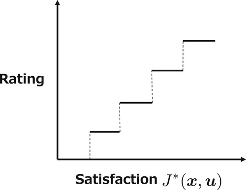
. An example of the user rating is realized by a questionnaire. The user gives m-grade evaluation based on his/her satisfaction with the control system as illustrated in Figure .
Figure 1. An example of user rating: five-grade evaluation is given to the control system, such as Excellent/Very Good/Good/Average/Poor.
Recall that in control system , controller K pursues the performance in the sense of the estimated objective function
, parameterized by
, to give experience
to the user. There exists a gap in the estimated utility
and true utility
. We assume that the user rating depends on the gap: the user rates the control system high (low) if the gap is small (large).
To model the user rating, we define the gap in the utility gained from experience as
(2)
(2) Based on (Equation2
(2)
(2) ), the user rating r is modelled by a piecewise constant function as
(3)
(3)
where are positive constants satisfying
, and
are also positive constants that indicate the range of existence of
. One can assume the rating as
for six-grade evaluation. In this setting, since the value of r is quantized, controller K cannot access the exact value of
.
Remark 2.1
holds since
. This fact is used for the analysis given in Section 4.
We impose a technical assumption on the model of the system-user, denoted by H. In addition to user rating r, system-user H gives the sign of to the control system based on his/her experience
. Then, the model of H is described by
(4)
(4) where
is the sign function. We see that this R is a “reward” in the reinforcement learning framework. Controller K can access reward R, which depends on user-experience
, to estimate
and to update its control law.
Remark 2.2
A similar problem of estimating objective functions and/or rewards, which generate the control actions, is known as inverse reinforcement learning (IRL). See e.g. [Citation12,Citation13] for the problem setting and e.g. [Citation14–16] for its applications. In most of the IRL frameworks, the control law is pre-defined and fixed, and its generating data is available for the estimation. On the other hand, in this paper, the control law is not fixed and to be updated, and the rating of a system-user, who is not included in the control loop, is available.
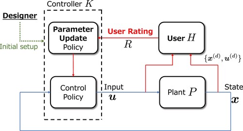
The block diagram of the control system with the user rating is illustrated in Figure . In the figure, the blue line connecting the controller and the plant indicates the loop of the control operation, while the red line connecting the user, controller, and plant indicates the loop of the controller update.
Figure 2. Personalized control system updated based on user rating.
2.3. Problem of controller update
Control system is updated based on user rating
. The flow of the update is given as follows.
Flow of controller update
The control system at version τ, denoted by
, is operated, and the user gains experience
The user gives his/her rating
Parameters
Control law K is updated based on the estimated objective function
The version of the control system is updated as
Note that control law K is uniquely determined once the parameter estimation is performed. This implies the essence of the controller update is the parameter estimation, addressed at Stage 3. The estimation problem is given as follows:
Problem 2.1
Given , estimate
.
3. Parameter estimation algorithm
In this section, we propose an algorithm of estimating parameters that characterize the user objective function given in (Equation1(1)
(1) ). To simplify the discussion, the objective function is characterized by only two parameters
and
, i.e.
The following discussion and the derived algorithm are extended to more general ℓ-parameters cases in a straightforward manner.
We aim at deriving the algorithm of estimating the parameters. Since the user rating is modelled by a quantized function as (Equation3(3)
(3) ), the parameter estimation can be reduced to a class of set-membership estimation [Citation17] as studied for state estimation problems [Citation18,Citation19]. Section 3.1 is devoted to the estimation of a parameter region. In Section 3.2, the parameter estimate is given from the region, and the estimation algorithm is presented.
3.1. Estimate of parameter region
Recall first that user rating R, given in (Equation4(4)
(4) ), includes rough information on his/her utility gained from experience
. We suppose that
holds for the experience, which implies the user gives s-grade for a current control system. Further supposing
, we have the following inequality
(5)
(5) where
. Further, we let
. Then, we see that
is described by
(6)
(6) where
and
are the estimated parameters at
th trial on the controller update. Then, by substituting (Equation6
(6)
(6) ) into (Equation5
(5)
(5) ), we have
(7)
(7) The set of the linear inequalities in (Equation7
(7)
(7) ) represents the existence region of
and
.
In a similar manner, supposing , we see that
(8)
(8) holds.
Consider again the τth trial on the controller update for derive the parameter estimate algorithm: a control operation is performed, and the system-user rates the control system based on his/her experience
. We suppose here that in the rating
,
holds, i.e. the user rates the system by s-grade. Then, letting
(9)
(9) Recalling the user rating given at the first to
th control operations, we show that
where
(10)
(10) and
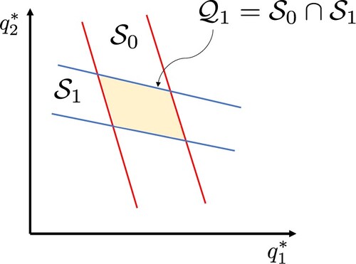
the initial guess on the parameter region. The update of the parameter existence region is illustrated in Figure . In the figure, the region enclosed by the red line is
, and the region enclosed by the blue line is
. The coloured area represents the parameter existence region
. In this way, we contract the parameter existence region by taking the intersection repeatedly. In the next subsection, we define the parameter estimate
from
.
Figure 3. Estimate of parameter existence region.
3.2. Update method of estimated parameters
One can define the estimate by the “centre” of region
. A drawback of taking the centre is its complexity: when the number of the controller update increases, i.e. τ increases, it is difficult to find the centre from
of (Equation10
(10)
(10) ), which is a polytope. To find the estimate
in a computationally tractable way, we apply an approximation of
. Let
be the rectangle region that approximates
, and is defined by
(11)
(11) where
and
are defined by
respectively. Note that region
is an “outer” approximation of
, i.e. it holds that
By taking the approximation of
as (Equation11
(11)
(11) ) at every controller update τ, we can find the estimate
in a simplified manner as
(12)
(12) where
represents the centre of gravity, i.e.
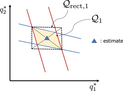
The approximation of the parameter existence region and parameter estimate in (Equation12
(12)
(12) ) are illustrated in Figure . In the figure, the black dotted line represents the rectangle region
while the blue triangle represents the estimated parameters
.
Figure 4. Outer approximation of to define
, and the centre of
to define
.
Finally, the algorithm of estimating parameters is summarized in Algorithm 1.

4. Analysis of algorithm
In this section, we address the convergence analysis of the proposed algorithm. We present the following theorem, which states the contraction of region .
Theorem 4.1
In Algorithm 1, it holds that
(13)
(13) where
represents the volume of S.
Proof.
We consider that by the user rating,
(14)
(14) holds for some
and
is obtained as
Consider here the following two cases:
and
in user rating R. First, suppose
implying that (Equation14
(14)
(14) ) is reduced to
.
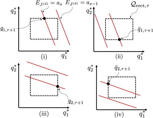
To prove (Equation13(13)
(13) ), we show that one of the following four conditions holds.
(15)
(15) The graphical interpretation of conditions (i)–(iv) is given in Figure . We see that (i) holds if and only if line
intersects segment
, which is a part of the boundary of
. In the same way as the derivation of (Equation7
(7)
(7) ) from (Equation5
(5)
(5) ), the condition for the intersection is described by
where
In a similar manner, (ii)–(iv) are equivalently reduced to
respectively, where
Now, we suppose that none of (i)
–(iv)
holds to prove (Equation13
(13)
(13) ) by contradiction. Then, it follows that both of the following inequalities
hold. then, we have
Here, we note that
must hold since
and
. This contradicts that none of (i)
–(iv)
holds.
Figure 5. Condition for contraction, given in (Equation15(15)
(15) ).
Next, we consider the case , which implies that (Equation14
(14)
(14) ) is reduced to
.
In the same way as the case of , to prove (Equation13
(13)
(13) ), we show that one of the following conditions holds.
where
Supposing that none of (i)
–(iv)
holds, we have
Recall
as stated in Remark 2.1. It follows that
holds. Consequently, it holds that
This contradicts that none of (i)
–(iv)
holds. This concludes the statement of the theorem holds.
Remark 4.1
As implied by Theorem 4.1, by iterating the controller update with Algorithm 1, the parameter region contracts monotonically in the sense of the outer approximation. The asymptotic convergence of
to
is not guaranteed in the analysis but is numerically verified in a demonstration given in Section 5.
5. Numerical experiment
In this section, we present a numerical experiment of the proposed control system with Algorithm 1. In the experiment, we demonstrate personalization using the proposed control system, considering two users.
5.1. Problem setting
We address the LQR problem. A plant system is given by a discrete-time linear state space equation:
(16)
(16) where system matrices A and B are given by
The objective function of a system-user is described by
where Q and W are weighting matrices. The corresponding optimal control law is given by
(17)
(17) where
is the optimal feedback gain and P is the solution to the Riccati equation
. We consider two users, user A and user B. The parameters in J for user A are given by
and W = 5. Then, the parameters for user B are given by
and W = 5.
It should be noted again that J is private, i.e. the system-designer cannot access Q directly. In this experiment, we try to estimate and
based on the following user rating;
(18)
(18) The flow of the experiment is shown below.
Set some initial estimate
A control experiment is performed where the initial state
A system-user evaluates the temporal control system and gives a rating to a system-designer based on (Equation18
Apply Algorithm 1 to the user rating to update the estimate of
Update control law (Equation17
Back to Stage 2.
The experiment was performed under , which is the initial guess.
5.2. Experiment results
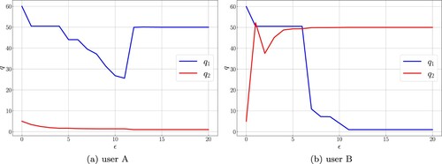
The result of the experiment is given in Figures . The transitions of the parameters and
obtained from the experiment are shown in Figure . In the figure, the horizontal axis represents the number of parameter updates ϵ and the vertical axis represents the parameter value. We see that the parameter estimate
converges to
for user A, and to
for user B.
Figure 6. Transitions of parameter estimate. (a) user A and (b) user B.
Next, the transitions of the user rating are shown in Figure . In the figure, the horizontal axis represents the number of parameter updates ϵ and the vertical axis represents the value of the utility gained from the control system. For either user A or B, we see that the utility is maximized by the algorithm even if the system-designer cannot access full information on the objective function.
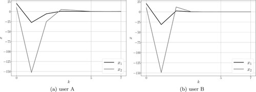
Finally, we show the state transitions of personalized control systems in Figure , which use converged estimated parameters for the control. In the figure, the horizontal axis represents the discrete-time k and the vertical axis represents the state of the plant system (Equation16(16)
(16) ). We see that the control behaviour is different for each user, which indicates that the control system is personalized.
Figure 7. Transitions of utility. (a) user A and (b) user B.
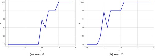
Figure 8. State transitions of personalized control system. (a) user A and (b) user B.
6. Conclusion
In this paper, we addressed the personalization of control systems where the optimal controller is updated according to users' private objective. We formulated a problem of estimating the individual objective function based on the user ratings and proposed its solution algorithm. The algorithm was analysed for a special case where the objective function is characterized by only two parameters. Finally, a numerical experiment showed the usefulness of the algorithm.
We have not proved that Theorem 4.1 holds for the case with more than three parameters, so future works include the extension of the analysis where a general objective function is addressed. Another future work is to model the user rating in a different manner to (Equation3(3)
(3) ).
Disclosure statement
No potential conflict of interest was reported by the author(s).
Additional information
Funding
Notes on contributors
Tomotaka Nii
Tomotaka Nii received the B.E. degrees in the Department of Applied Physico-informatics from Keio University in 2022. His research interests include control theory for human-in-the-loop systems.
Masaki Inoue
Masaki Inoue received the M.E. and Ph.D. degrees in mechanical engineering from Osaka University in 2009 and 2012, respectively. He served as a Research Fellow of the Japan Society for the Promotion of Science from 2010 to 2012. From 2012 to 2014, he was a Project Researcher of FIRST, Aihara Innovative Mathematical Modelling Project, and also a Doctoral Researcher of the Graduate School of Information Science and Engineering, Tokyo Institute of Technology. Currently, he is an Associate Professor of the Department of Applied Physico-informatics, Keio University. His research interests include control theory for human-in-the-loop systems. He is a member of IEEE, SICE, and ISCIE.
References
- Fan H, Poole MS. What is personalization? Perspectives on the design and implementation of personalization in information systems. J Organ Comput Electron Commer. 2006;16(3–4):179–202.
- Tuzhilin A. Personalization: the state of the art and future directions. Bus Comput. 2009;3(3):3–43.
- Hasenjager M, Heckmann M, Wersing H. A survey of personalization for advanced driver assistance systems. IEEE Trans Intell Veh. 2020;5(2):335–344.
- Yi D, Su J, Hu L, et al. Implicit personalization in driving assistance: state-of-the-art and open issues. IEEE Trans Intell Veh. 2019;5(3):397–413.
- Lu C, Gong J, Lv C, et al. A personalized behavior learning system for human-like longitudinal speed control of autonomous vehicles. Sensors. 2019;19(17):3672.
- Noto N, Okuda H, Tazaki Y, et al. Steering assisting system for obstacle avoidance based on personalized potential field. In: 2012 15th International IEEE Conference on Intelligent Transportation Systems. IEEE; 2012. p. 1702–1707.
- Wiering MA, Van Otterlo M. Reinforcement learning. Adapt Learn Optim. 2012;12(3):729.
- Lewis FL, Vrabie D, Vamvoudakis KG. Reinforcement learning and feedback control: using natural decision methods to design optimal adaptive controllers. IEEE Contr Syst Mag. 2012;32(6):76–105.
- Kiumarsi B, Vamvoudakis KG, Modares H, et al. Optimal and autonomous control using reinforcement learning: a survey. IEEE Trans Neural Netw Learn Syst. 2018;29(6):2042–2062.
- Zanon M, Gros S, Bemporad A. Practical reinforcement learning of stabilizing economic MPC. In: 2019 18th European Control Conference (ECC), Naples; 2019. p. 2258–2263.
- Ernst D, Glavic M, Capitanescu F, et al. Reinforcement learning versus model predictive control: a comparison on a power system problem. IEEE Trans Syst Man Cybern B. 2009;39(2):517–529.
- Ng AY, Russell S. Algorithms for inverse reinforcement learning. In: International Conference on Machine Learning, Stanford, CA; Vol. 1; 2000. p. 2.
- Arora S, Doshi P. A survey of inverse reinforcement learning: challenges, methods and progress. Artif Intell. 2021;297:Article ID 103500.
- Ozkan MF, Ma Y. Modeling driver behavior in car-following interactions with automated and human-driven vehicles and energy efficiency evaluation. IEEE Access. 2021;9:64696–64707.
- Ozkan MF, Rocque AJ, Ma Y. Inverse reinforcement learning based stochastic driver behavior learning. IFAC-PapersOnLine. 2021;54(20):882–888.
- Ozkan MF, Ma Y. Personalized adaptive cruise control and impacts on mixed traffic. In: 2021 American Control Conference (ACC), New Orleans; 2021. p. 412–417.
- Milanese M, Vicino A. Optimal estimation theory for dynamic systems with set membership uncertainty: an overview. Automatica. 1991;27(6):997–1009.
- Savkin AV, Petersen IR. Set-valued state estimation via a limited capacity communication channel. IEEE Trans Automat Contr. 2003;48(4):676–680.
- Shi D, Chen T, Shi L. On set-valued kalman filtering and its application to event-based state estimation. IEEE Trans Automat Control. 2015;60(5):1275–1290.