Self-triggered output synchronization of heterogeneous linear agents through a cloud repository

ABSTRACT

This paper deals with a self-triggered output synchronization control method of a heterogeneous linear multi-agent system through a cloud repository. In the cloud-mediated self-triggered control approach, each agent asynchronously accesses the cloud repository to get past information on its neighbouring agents. The proposed controller consists of a virtual exosystem (VE) and a local tracking controller, where the VE is driven by an input based on the neighbours' information stored in the cloud. At the access time, each agent predicts future behaviours of the VEs' states incorporated in its neighbouring agents as well as of its own VE and locally determines its next access time to the cloud. Different from conventional self-triggered control methods, each agent cannot instantaneously communicate with its neighbouring agents at every triggering time. In this paper, we introduce an output synchronizing controller design method through a cloud repository which can cope with difficulties caused by non-instantaneous communications through the cloud repository. As the main result, we prove that the proposed self-triggered controller achieves the bounded output synchronization of the closed-loop system without exhibiting any Zeno behaviours.

KEYWORDS:

• Self-triggered control
• cloud-mediated control
• output synchronization
• bounded synchronization
• heterogeneous multi-agent systems

1. Introduction

Coordination of a multi-agent system is one of the central topics in the recent control engineering field due to the wide range of its applications. In a multi-agent system, each agent autonomously acts through interaction with its neighbouring agents, and the whole system achieves various cooperative tasks such as consensus and synchronization [1–5].

In the last decade, event-triggered control and self-triggered control have been extensively studied in the literature [6,7]. In the event-triggered control strategy, each agent executes information exchange only when a prescribed triggering condition is satisfied. Moreover, the self-triggered controller computes the next triggering time based on the prediction of future behaviours of the neighbouring agents (see [8,9] and the references therein). Most of the event-triggered controllers employed a peer-to-peer (P2P) communication scheme between agents [10,11]. The P2P information exchange is practically carried out by wireless communication with geographically neighbouring agents.

As another research direction, self-triggered coordination via a cloud repository has been reported, which does not require the inter-agent P2P communication. In the control schemes using a cloud repository (hereafter, we simply call it “cloud”), each agent asynchronously accesses the cloud to get past information on its neighbouring agents. Then, the agent predicts future behaviours of the neighbouring agents as well as of its own, and locally determines its next access time to the cloud. It may be noticed that the cloud-mediated approach preserves the benefit of the self-triggered control which does not require the continuous monitoring of the triggering condition.

Self-triggered control through a cloud is especially effective in the situation where the instantaneous communication between the agents is not possible. An application of such a control scheme is a cooperative control of autonomous underwater vehicles (AUVs) as mentioned in [12–16]. Generally, it is difficult for each AUV to communicate with others under the water due to the poor ability of its IoT devices.

Another benefit of the cloud-mediated control is that each agent does not have to keep communication channels open (be listening) in order to detect the triggerings of its neighbouring agents. Such a situation can be typically found in a virtual power plant (VPP). The VPP consists of various distributed energy resources such as energy storages and small-scale generation units. In the VPP framework, the distributed energy resources are cooperatively controlled so that they provide energy as if they were a single large power plant. These resources are geographically distributed, and thus an IoT device attached to each distributed resource communicates with each other indirectly through a cloud rather than a direct wireless communication. Moreover, thanks to the intermittent communication through the cloud, the IoT devices can reduce power consumption and communication frequency. This improves implementability of the VPP in practical situations.

Adaldo et al. [12,13] proposed cloud-supported control techniques for consensus and trajectory tracking in the presence of disturbances. In these works, the agent dynamics was modelled as a single integrator. Nowzari and Pappas [14] and Bowman, Nowzari, and Pappas [15] proposed self-triggered control methods through a cloud for the consensus problem under the assumption that the dynamics of each agent is the scalar integrator. In a formation control problem, Adaldo et al. [16] extended the previous results in the case of the single integrator to the case of a double integrator. Namba and Takaba [17–19] proposed the cloud-mediated self-triggered state synchronizing control methods of homogeneous linear agents. However, the individual dynamics may be different from the others.

For heterogeneous nonlinear agents, the only recent publication by Hong and Zhang [20] reported a leader-following state synchronization controller design based on the cloud-based self-triggered fashion. Although Hong and Zhang [20] dealt with heterogeneous agents, it was assumed that the state dimensions of all agents are equal, and that the leader is a single integrator. Therefore, the method in [20] is not applicable to neither linear systems with heterogeneous state dimensions nor leaderless synchronization problems.

Output synchronization is a generalization of the synchronization problem which aims at synchronization of evaluated outputs rather than the states themselves. The agent dynamics can be heterogeneous, and the state dimension of each agent is possibly different from others. In early papers, Wieland and Allgöwer [21], and Wieland, Sepulchre, and Allgöwer [22] showed that the internal model principle plays a crucial role in the output synchronization problem of the heterogeneous multi-agent system. Along this line, Hu, Liu, and Feng [23] and Almeida, Silvestre, and Pascoal [24] proposed the event-triggered and self-triggered algorithms for the output synchronization of the heterogeneous linear agents. The references [23,24] assumed that the instantaneous communication between the agents is available, and thus each agent has to be listening to the triggerings of its neighbours. To the best of the author's knowledge, there have not been reported any results utilizing cloud-mediated self-triggering strategy.

In this paper, we will consider a self-triggered synchronization control method for a heterogeneous linear multi-agent system through the cloud. This is the first paper which reports the cloud-mediated self-triggered control method for the output synchronization problem of a heterogeneous multi-agent system. As the contribution of this paper, the present results substantially spread the class of linear multi-agent systems to which the cloud-mediated approach is applicable. We reduce the output synchronization of the heterogeneous agents to the combination of the state synchronization of homogeneous virtual exosystems (VE) and the local tracking control based on the design procedure in [22]. The proposed self-triggered controller consists of the virtual exosystem and the local output tracking controller. The virtual exosystems communicate with each other through the cloud in an asynchronous self-triggered fashion, and the outputs of all the agents achieve bounded synchronization within the specified tolerance.

Notational Conventions

We denote the N dimensional all-ones vector by ${\text{𝟙}}_N:=[1,\dots ,1{]}^{\mathsf{\text{T}}}$. $I_N$ is the $N\times N$ identity matrix. Closed and open intervals are denoted by $[a,b]$ and $]a,b[$, respectively (We use the similar notation for half-open intervals). $X\otimes Y$ denotes the Kronecker product of X and Y. The spectrum of the matrix M is denoted by $\sigma \left(M\right)$.

2. Problem formulation

2.1. Heterogeneous agent dynamics

Consider N heterogeneous linear multi-agent system whose dynamics is given by (1) $\begin{array}{rl}{\dot{x}}_i\left(t\right)& =A_i{x}_i\left(t\right)+B_i{u}_i\left(t\right)\end{array}$(1) (2) $\begin{array}{rl}{y}_i\left(t\right)& =C_i{x}_i,i=1,2,\dots ,N\end{array}$(2) where $x_i\left(t\right)\in {\mathbb{R}}^{n_i}$ is the state, $u_i\left(t\right)\in {\mathbb{R}}^{m_i}$ is the input, $y_i\left(t\right)\in {\mathbb{R}}^p$ is the evaluated output, and $A_i\in {\mathbb{R}}^{n_i\times n_i},B_i\in {\mathbb{R}}^{n_i\times m_i},C_i\in {\mathbb{R}}^{p\times n_i}$ are the constant matrices. We make the following assumption for later discussion.

Assumption 2.1

The pair $(A_i,B_i)$ is stabilizable, and the pair $(C_i,A_i)$ is detectable.

2.2. Communication model

2.2.1. Cloud repository

In this subsection, we introduce the model of a cloud repository due to [13,14]. We consider the situation where each agent communicates with its neighbours using a cloud. It should be noted that the cloud only stores information of all the agents, and does not execute any computation. The term “access” means the entire process consisting of connections, downloading/uploading, and disconnections. We assume that these operations are instantaneously executed. As described in subsection 2.3, the virtual exosystem is embedded in each agent's controller. Each agent uploads and downloads the states and inputs of the VE's at it's access time instants, which are denoted by ${\zeta }_i\left(t_i^{l_i}\right)$ and $v_i\left(t_i^{l_i}\right)$, respectively.

The cloud stores information described in Table 1. We denote the latest access time of the agent i by $t_i^{l_i\left(t\right)}$ at the current access time t, where $l_i\left(t\right)$ indicates how many times the agent i connected to the cloud before and at the time t. We often write $t_i^{l_i}$ by dropping the current time for simplicity. Figure 1 illustrates the relation among these access times.

Figure 1. Illustration of the relation among the access times of the agents i and j.

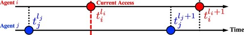
Table 1. Information stored in the cloud at t.

Agents	$\mathbf{1}$	$\mathbf{2}$	···	$\mathit{N}$
The last access time	$t_1^{l_1}$	$t_2^{l_2}$	···	$t_N^{l_N}$
The last access state of the VE	${\zeta }_1\left(t_1^{l_1}\right)$	${\zeta }_2\left(t_2^{l_2}\right)$	···	${\zeta }_N\left(t_N^{l_N}\right)$
The input of the VE	$v_1\left(t_1^{l_1}\right)$	$v_2\left(t_2^{l_2}\right)$	···	$v_N\left(t_N^{l_N}\right)$
The next access time	$t_1^{l_1+1}$	$t_2^{l_2+1}$	···	$t_N^{l_N+1}$

It may be noted that each agent does not have to store the information on its state $x_i\left(t_i^{l_i}\right)$ as well as its control input $u_i\left(t_i^{l_i}\right)$.

2.2.2. Accessibility graph

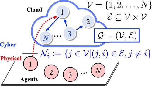
Throughout this paper, it is assumed that each agent can only access the information of predetermined agents among the information stored in the cloud repository. Though one may think that each agent should be able to access all the information in the cloud, we make this assumption from the viewpoint of privacy protection. We employ a directed graph to describe which agents can be accessed by each agent. It may be noted that a mathematical graph has been widely used for describing communications between agents in conventional multi-agent systems (see e.g. [25]). In this section, we briefly review the fundamentals of the algebraic graph theory which will be useful in this paper.

The accessibility between agents is modelled by a directed graph, which is defined as a pair $\mathcal{G}=(\mathcal{V},\mathcal{E})$, where $\mathcal{V}:=\{1,2,\dots ,N\}$ is a vertex set and $\mathcal{E}\subseteq \mathcal{V}\times \mathcal{V}$ is an edge set. Each vertex represents an agent and an edge $(j,i)\in \mathcal{E}$ means that the vertex i can receive the information from the vertex j. The overall communication model is depicted in Figure 2.

Figure 2. Communication model.

We make the following assumption.

Assumption 2.2

1. The graph $\mathcal{G}$ has a directed spanning-tree.

2. The topology of the graph $\mathcal{G}$ is time-invariant.

We define the neighbour set of the agent i by ${\mathcal{N}}_i:=\{j\in \mathcal{V}|(j,i)\in \mathcal{E},j\ne i\}.$We also define the graph Laplacian by $\begin{array}{r}L=\left[{\ell }_{ij}\right],\text{where}{\ell }_{ij}:=\{\begin{array}{ll}|{\mathcal{N}}_i|& i=j\\ -1& (j,i)\in \mathcal{E}\\ 0& \text{otherwise}.\end{array}\end{array}$As is well known, the following fact holds true under Assumption 2.2 [25].

Fact 2.1

1. $\mathrm{r}\mathrm{a}\mathrm{n}\mathrm{k}L=N-1$, namely, L has only one zero eigenvalue.

2. ${\text{𝟙}}_N$ is the right eigenvector of the zero eigenvalue, namely, $L{\text{𝟙}}_N=0$.

For later discussion, let ${\varphi }^{\mathsf{\text{T}}}$ be the left eigenvector of the zero eigenvalue for L such that ${\varphi }^{\mathsf{\text{T}}}{\text{𝟙}}_N=1$. It is seen from Gershgorin's disk theorem and the definition of L that all the nonzero eigenvalues of L have positive real parts. Hence, under Assumption 2.2 we denote the eigenvalues of L with ${\lambda }_1,{\lambda }_2,\dots ,{\lambda }_N$ in the ascending order with respect to their real parts ${\lambda }_1=0<\mathrm{R}\mathrm{e}\left({\lambda }_2\right)\le \mathrm{R}\mathrm{e}\left({\lambda }_3\right)\le \cdots \le \mathrm{R}\mathrm{e}\left({\lambda }_N\right).$Choose the constant matrices $X_1$ and $X_2$ such that $U:=\left[\begin{array}{cc}{\text{𝟙}}_N& X_1\end{array}\right],U^{-1}:=\left[\begin{array}{c}{\varphi }^{\mathsf{\text{T}}}\\ X_2\end{array}\right].$This implies that (3) $\begin{array}{r}{U}^{-1}LU=\left[\begin{array}{cc}0& 0\\ 0& X_{2}L{X}_1\end{array}\right]=\left[\begin{array}{cc}0& 0\\ 0& \check{L}\end{array}\right].\end{array}$(3) It should be noted that the eigenvalues of $\check{L}$ are equal to ${\lambda }_2,\dots ,{\lambda }_N$.

2.3. Control objective and controller structure

This paper is concerned with the bounded output synchronization problem where the outputs of all agents should remain close to each other within a prescribed tolerance in the steady state. In particular, we wish to synthesize a self-triggered controller which achieves the bounded output synchronization through asynchronous communication with the cloud. The formal statement of the problem will be provided below.

For the ith agent, we introduce the controller structure consisting of the following three components [22]: (4) $\begin{array}{rl}{\dot{\zeta }}_i\left(t\right)& =S{\zeta }_i\left(t\right)+v_i\left(t\right),\end{array}$(4) (5) $\begin{array}{rl}{\dot{\hat{x}}}_i\left(t\right)& =A_i{\hat{x}}_i\left(t\right)+B_i{u}_i\left(t\right)+L_i\left(C_i{\hat{x}}_i\right(t)-y_i(t\left)\right),\end{array}$(5) (6) $\begin{array}{rl}{u}_i\left(t\right)& =K_i\left({\hat{x}}_i\right(t)-{\mathrm{\Pi }}_i{\zeta }_i(t\left)\right)+{\mathrm{\Gamma }}_i{\zeta }_i\left(t\right),\end{array}$(6) where ${\zeta }_i\left(t\right)\in {\mathbb{R}}^q$ is the state of the virtual exosystem, ${\hat{x}}_i\left(t\right)\in {\mathbb{R}}^{n_i}$ is the estimated state, $S\in {\mathbb{R}}^{q\times q},L_i\in {\mathbb{R}}^{n_i\times p},K_i\in {\mathbb{R}}^{m_i\times n_i},{\mathrm{\Pi }}_i\in {\mathbb{R}}^{n_i\times q},{\mathrm{\Gamma }}_i\in {\mathbb{R}}^{m_i\times q}$ are the constant matrices. Equations (4(4) $\begin{array}{rl}{\dot{\zeta }}_i\left(t\right)& =S{\zeta }_i\left(t\right)+v_i\left(t\right),\end{array}$(4) ), (5(5) $\begin{array}{rl}{\dot{\hat{x}}}_i\left(t\right)& =A_i{\hat{x}}_i\left(t\right)+B_i{u}_i\left(t\right)+L_i\left(C_i{\hat{x}}_i\right(t)-y_i(t\left)\right),\end{array}$(5) ), and (6(6) $\begin{array}{rl}{u}_i\left(t\right)& =K_i\left({\hat{x}}_i\right(t)-{\mathrm{\Pi }}_i{\zeta }_i(t\left)\right)+{\mathrm{\Gamma }}_i{\zeta }_i\left(t\right),\end{array}$(6) ) correspond to the Virtual Exosystem (VE), the observer, and the local tracking controller, respectively.

Assumption 2.3

The matrices $A_i+B_i{K}_i,A_i+L_i{C}_i,i=1,\dots ,N$ are Hurwitz stable.

To design $K_i$ and $L_i$ so that Assumption 2.3 is satisfied, one can use pole placement methods for the design of $K_i$ and $L_i$. It should be noted that, under Assumption 2.3, there exist ${\lambda }_{{ϵ}_i}>0$, ${\kappa }_{{ϵ}_i}>0$, ${\lambda }_{{\tilde{x}}_i}>0$, and ${\kappa }_{{\tilde{x}}_i}>0$ satisfying (7) $\begin{array}{rl}\Vert {\mathrm{e}}^{(A_i+B_i{K}_i)t}\Vert & \le {\kappa }_{{ϵ}_i}{\mathrm{e}}^{-{\lambda }_{{ϵ}_i}t},\mathrm{\forall }t\ge 0\end{array}$(7) (8) $\begin{array}{rl}\Vert {\mathrm{e}}^{(A_i+L_i{C}_i)t}\Vert & \le {\kappa }_{{\tilde{x}}_i}{\mathrm{e}}^{-{\lambda }_{{\tilde{x}}_i}t},\mathrm{\forall }t\ge 0,\end{array}$(8) respectively (Also refer to Remark 3.2).

The structure of the self-triggered output synchronizing controller for the ith agent is depicted in Figure 3. The physical dynamics of the agent corresponds to the grey block in Figure 3.

Figure 3. The controller and agent dynamics of the ith agent.

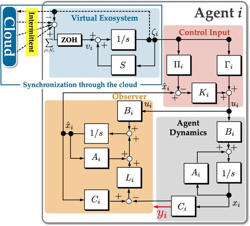
The VE plays an important role in the controller, which generates the reference signal to be tracked by the output $y_i$. Actually, the VE is also called the reference generator [24] (For more detail, refer to Assumption 2.4 and Remark 2.2). In this paper, we assume that each agent exchanges the local state of the VE with the neighbours through the cloud aiming at the output synchronization. In this sense, the output synchronization of the heterogeneous multi-agents can be reduced to the self-triggered state synchronization problem of the VEs through the cloud (the blue part in Figure 3) and the local tracking problem to the individual VE trajectory (the red part in Figure 3). Thanks to this structure, we can separately design the cloud-mediated self-triggered synchronizing controller of the VEs and the local tracking controller.

Remark 2.1

The VE in (4(4) $\begin{array}{rl}{\dot{\zeta }}_i\left(t\right)& =S{\zeta }_i\left(t\right)+v_i\left(t\right),\end{array}$(4) ) is driven by the piecewise constant input based on the intermittent self-triggered communication through the cloud whereas the observer and the local tracking controller (5(5) $\begin{array}{rl}{\dot{\hat{x}}}_i\left(t\right)& =A_i{\hat{x}}_i\left(t\right)+B_i{u}_i\left(t\right)+L_i\left(C_i{\hat{x}}_i\right(t)-y_i(t\left)\right),\end{array}$(5) )–(6(6) $\begin{array}{rl}{u}_i\left(t\right)& =K_i\left({\hat{x}}_i\right(t)-{\mathrm{\Pi }}_i{\zeta }_i(t\left)\right)+{\mathrm{\Gamma }}_i{\zeta }_i\left(t\right),\end{array}$(6) ) are exactly continuous-time systems. It should also be noted that the agent i can continuously obtain the state ${\zeta }_i$ of its VE even though its own state $x_i$ is not measurable. This is a reasonable assumption because the VEs are artificially designed and embedded into the synchronizing controllers. In this paper, we also assume that the output $y_i$ is continuously measurable by the agent i.

We make the following assumption that is standard in the literature [22–24].

Assumption 2.4

There exist a constant q and constant matrices $S\in {\mathbb{R}}^{q\times q}$, $R\in {\mathbb{R}}^{p\times q}$, ${\mathrm{\Pi }}_i\in {\mathbb{R}}^{n_i\times q}$, ${\mathrm{\Gamma }}_i\in {\mathbb{R}}^{m_i\times q}$ satisfying (9(9) $\begin{array}{rl}{A}_i{\mathrm{\Pi }}_i+B_i{\mathrm{\Gamma }}_i& ={\mathrm{\Pi }}_{i}S\end{array}$(9) ), (10(10) $\begin{array}{rl}{C}_i{\mathrm{\Pi }}_i& =R\end{array}$(10) ), and the pair $(R,S)$ is detectable. (9) $\begin{array}{rl}{A}_i{\mathrm{\Pi }}_i+B_i{\mathrm{\Gamma }}_i& ={\mathrm{\Pi }}_{i}S\end{array}$(9) (10) $\begin{array}{rl}{C}_i{\mathrm{\Pi }}_i& =R\end{array}$(10)

Remark 2.2

Equations (9(9) $\begin{array}{rl}{A}_i{\mathrm{\Pi }}_i+B_i{\mathrm{\Gamma }}_i& ={\mathrm{\Pi }}_{i}S\end{array}$(9) ) and (10(10) $\begin{array}{rl}{C}_i{\mathrm{\Pi }}_i& =R\end{array}$(10) ) are well known as the Francis' equation (refer to [26,27]). Due to the internal model principle for the multi-agent systems [21,22], the same internal model must be incorporated into every agent-controller pair in order to achieve the output synchronization. Actually, the internal model is characterized by the matrices S and R satisfying Assumption 2.4.

To design the control input to the VE incorporated in the ith agent, we firstly define the fictitious relative state feedback controller with ${\zeta }_i\left(t\right)$ and ${\zeta }_j\left(t\right)$, namely, $z_i\left(t\right)=F\sum _{j\in {\mathcal{N}}_i}\left({\zeta }_j\right(t)-{\zeta }_i(t\left)\right),$where $F\in {\mathbb{R}}^{q\times q}$ is the constant gain. As the input to the ith VE, by applying the Zeroth-Order Hold (ZOH) method to $z_i\left(t\right)$, we use (11) $v_i\left(t\right)=F\sum _{j\in {\mathcal{N}}_i}\left({\hat{\zeta }}_j^i\right(t_i^{l_i})-{\zeta }_i(t_i^{l_i}\left)\right),t\in [t_i^{l_i},t_i^{l_i+1}[,$(11) where ${\hat{\zeta }}_j^i$ denotes the prediction of ${\zeta }_j$ by the agent i which is given by (12) $\begin{array}{rl}& {\hat{\zeta }}_j^i\left(t\right)\\ & =\{\begin{array}{l}{\mathrm{e}}^{S(t-t_j^{l_j})}{\zeta }_j\left(t_j^{l_j}\right)\\ +{\displaystyle {\int }_{t_j^{l_j}}^t{\mathrm{e}}^{S(t-\tau )}{v}_j\left(t_j^{l_j}\right)\mathrm{d}\tau }& t\in [t_j^{l_j},t_j^{l_j+1\left(t_i^{l_i}\right)}],\\ {\mathrm{e}}^{S(t-t_j^{l_j+1})}{\hat{\zeta }}_j^i\left(t_j^{l_j+1\left(t_i^{l_i}\right)}\right)& t>t_j^{l_j+1\left(t_i^{l_i}\right)},\end{array}.\end{array}$(12) The predicted state ${\hat{\zeta }}_j^i\left(t_i^{l_i}\right)$ in $v_i\left(t\right)$, $t\in [t_i^{l_i},t_i^{l_i+1}[$ is computed by using the first equation in (12(12) $\begin{array}{rl}& {\hat{\zeta }}_j^i\left(t\right)\\ & =\{\begin{array}{l}{\mathrm{e}}^{S(t-t_j^{l_j})}{\zeta }_j\left(t_j^{l_j}\right)\\ +{\displaystyle {\int }_{t_j^{l_j}}^t{\mathrm{e}}^{S(t-\tau )}{v}_j\left(t_j^{l_j}\right)\mathrm{d}\tau }& t\in [t_j^{l_j},t_j^{l_j+1\left(t_i^{l_i}\right)}],\\ {\mathrm{e}}^{S(t-t_j^{l_j+1})}{\hat{\zeta }}_j^i\left(t_j^{l_j+1\left(t_i^{l_i}\right)}\right)& t>t_j^{l_j+1\left(t_i^{l_i}\right)},\end{array}.\end{array}$(12) ), i.e. ${\hat{\zeta }}_j^i\left(t_i^{l_i}\right)={\mathrm{e}}^{S(t_i^{l_i}-t_j^{l_j})}{\zeta }_j\left(t_j^{l_j}\right)+{\int }_{t_j^{l_j}}^{t_i^{l_i}}{\mathrm{e}}^{S(t-\tau )}{v}_j\left(t_j^{l_j}\right)\mathrm{d}\tau$. The input $v_i\left(t\right)$ can also be expressed as $v_i\left(t\right)=z_i\left(t_i^{l_i}\right),t\in [t_i^{l_i},t_i^{l_i+1}[$ under the situation where there is neither model uncertainty nor disturbances. The second equation in (12(12) $\begin{array}{rl}& {\hat{\zeta }}_j^i\left(t\right)\\ & =\{\begin{array}{l}{\mathrm{e}}^{S(t-t_j^{l_j})}{\zeta }_j\left(t_j^{l_j}\right)\\ +{\displaystyle {\int }_{t_j^{l_j}}^t{\mathrm{e}}^{S(t-\tau )}{v}_j\left(t_j^{l_j}\right)\mathrm{d}\tau }& t\in [t_j^{l_j},t_j^{l_j+1\left(t_i^{l_i}\right)}],\\ {\mathrm{e}}^{S(t-t_j^{l_j+1})}{\hat{\zeta }}_j^i\left(t_j^{l_j+1\left(t_i^{l_i}\right)}\right)& t>t_j^{l_j+1\left(t_i^{l_i}\right)},\end{array}.\end{array}$(12) ) will be used in the self-triggered access rule in the subsequent sections.

We denote the collection of all VEs' states and inputs by $\zeta :=\left[\begin{array}{c}{\zeta }_1\\ ⋮\\ {\zeta }_N\end{array}\right],v:=\left[\begin{array}{c}{v}_1\\ ⋮\\ v_N\end{array}\right]$respectively. Then the collective dynamics is given by (13) $\dot{\zeta }\left(t\right)=(S\otimes I_N)\zeta \left(t\right)+v\left(t\right).$(13) Let us define (14) $\begin{array}{rl}\alpha \left(t\right)& :=({\varphi }^{\mathsf{\text{T}}}\otimes I_q)\zeta \left(t\right),\end{array}$(14) (15) $\begin{array}{rl}{\delta }_i\left(t\right)& :={\zeta }_i\left(t\right)-\alpha \left(t\right).\end{array}$(15) We also denote $\delta :=[{\delta }_1^{\mathsf{\text{T}}},\dots ,{\delta }_N^{\mathsf{\text{T}}}{]}^{\mathsf{\text{T}}}$. To prove that the state synchronization of VEs is achieved, we will show that the VEs' states of all agents remain close to the signal $\alpha \left(t\right)$ within a prescribed tolerance in the steady state. Correspondingly, ${\delta }_i\left(t\right)$ is the VE's state deviation from $\alpha \left(t\right)$.

Based on the above preparation, we define the bounded output synchronization problem as follows.

Problem 2.1

Design a self-triggered distributed controller which satisfies (16) $\underset{t\to \mathrm{\infty }}{lim}sup\Vert y_i\left(t\right)-R\alpha \left(t\right)\Vert \le {\chi }_i^{\mathrm{o}\mathrm{u}\mathrm{t}},\mathrm{\forall }i\in \mathcal{V},$(16) for any initial states $x_i\left(0\right),i=1,2,\dots ,N$, where ${\chi }_i^{\mathrm{o}\mathrm{u}\mathrm{t}}$ denotes the desired tolerance which is given a priori by the designer for the agent i.

3. Cloud-mediated self-triggered output synchronization

This section will propose a self-triggered distributed controller through the cloud for the aforementioned output synchronization problem. Firstly, we will focus on the VE, and derive a triggering rule (access rule) which does not lead to any Zeno behaviour. Next, we will analyse the convergence property of the closed-loop system as the main result of this paper, and show that the output synchronization is achieved in the sense of (16(16) $\underset{t\to \mathrm{\infty }}{lim}sup\Vert y_i\left(t\right)-R\alpha \left(t\right)\Vert \le {\chi }_i^{\mathrm{o}\mathrm{u}\mathrm{t}},\mathrm{\forall }i\in \mathcal{V},$(16) ).

3.1. Cloud-mediated synchronization of the VEs

In this subsection, we briefly review the self-triggered synchronization of the homogeneous linear multi-agent system due to Namba and Takaba [18].

Define the input error by (17) ${\tilde{v}}_i\left(t\right):=v_i\left(t\right)-z_i\left(t\right).$(17) The collective dynamics (13(13) $\dot{\zeta }\left(t\right)=(S\otimes I_N)\zeta \left(t\right)+v\left(t\right).$(13) ) is expressed as (18) $\dot{\zeta }\left(t\right)=(I_N\otimes S-L\otimes F)\zeta \left(t\right)+I_N\tilde{v}\left(t\right),$(18) where $\tilde{v}:=\left[\begin{array}{c}{\tilde{v}}_1\\ ⋮\\ {\tilde{v}}_N\end{array}\right].$It follows from (14(14) $\begin{array}{rl}\alpha \left(t\right)& :=({\varphi }^{\mathsf{\text{T}}}\otimes I_q)\zeta \left(t\right),\end{array}$(14) ), (18(18) $\dot{\zeta }\left(t\right)=(I_N\otimes S-L\otimes F)\zeta \left(t\right)+I_N\tilde{v}\left(t\right),$(18) ) and ${\varphi }^{\mathsf{\text{T}}}L=0$ that (19) $\dot{\alpha }\left(t\right)=S\alpha \left(t\right)+({\varphi }^{\mathsf{\text{T}}}\otimes I_q)\tilde{v}\left(t\right).$(19) The dynamics of δ is then expressed as (20) $\dot{\delta }\left(t\right)=\mathcal{S}\delta \left(t\right)+{\mathcal{B}}^{\prime }\tilde{v}\left(t\right),$(20) where $\mathcal{S}:=I_N\otimes S-L\otimes F,{\mathcal{B}}^{\prime }:=(I_N-{\text{𝟙}}_N{\varphi }^{\mathsf{\text{T}}})\otimes I_q.$By recalling (3(3) $\begin{array}{r}{U}^{-1}LU=\left[\begin{array}{cc}0& 0\\ 0& X_{2}L{X}_1\end{array}\right]=\left[\begin{array}{cc}0& 0\\ 0& \check{L}\end{array}\right].\end{array}$(3) ), we can verify that $\begin{array}{r}\mathcal{S}=(U\otimes I_q)\left[\begin{array}{cc}0& 0\\ 0& \check{\mathcal{S}}\end{array}\right](U\otimes I_q{)}^{-1},\end{array}$where (21) $\check{\mathcal{S}}:=I_{N-1}\otimes S-\check{L}\otimes F.$(21) It may be noted that the stability of $\check{\mathcal{S}}$ plays a crucial role in the design of the synchronizing control law. To be more precise, we can easily show that $\check{\mathcal{S}}$ is Hurwitz stable if and only if $S-{\lambda }_{i}F$ is Hurwitz stable for $i=2,\dots ,N$.

Assumption 3.1

The matrices $S-{\lambda }_{i}F,i=2,\dots ,N$ are Hurwitz stable.

It may be noted that one can get a gain F satisfying Assumption 3.1 by solving a certain algebraic Riccati equation (refer to e.g. [28]).

Lemma 3.1 states that if the input error is smaller than or equal to the threshold in some interval, the input and the synchronization error can be upper bounded by some functions ${\mu }_i\left(t\right)$ and $\eta \left(t\right)$ over the same interval, respectively. We use these bounds in the design of the triggering function in the access rule in Lemma 3.2.

Lemma 3.1

[18]

Assume that (22) $\Vert {\tilde{v}}_i\left(t\right)\Vert \le s\left(t\right),\mathrm{\forall }i\in \mathcal{V}$(22) is satisfied for all t in some interval $[t_0,t_f[$, where (23) $s\left(t\right):=s_{\mathrm{\infty }}+(s_0-s_{\mathrm{\infty }}){\mathrm{e}}^{-{\lambda }_{s}t},$(23) with $s_0\ge s_{\mathrm{\infty }}>0$, ${\lambda }_s>0$. Then, the following inequalities hold. (24) $\begin{array}{rl}& \Vert \delta \left(t\right)\Vert \le \eta \left(t\right),\mathrm{\forall }t\in [t_0,t_f[,\end{array}$(24) (25) $\begin{array}{rl}& \Vert v_j\left(t\right)\Vert \le {\mu }_j\left(t\right),\mathrm{\forall }j\in \mathcal{V},\mathrm{\forall }t\in [t_0,t_f[,\end{array}$(25) with (26) $\begin{array}{rl}\eta \left(t\right)& :=\kappa {\mathrm{e}}^{-\lambda (t-t_0)}{\eta }_0\\ & +\kappa \sqrt{N}\Vert {\mathcal{B}}^{\prime }\Vert {\int }_{t_0}^t{\mathrm{e}}^{-\lambda (t-\tau )}s\left(\tau \right)\mathrm{d}\tau ,\end{array}$(26) (27) $\begin{array}{rl}{\mu }_j\left(t\right)& :={\text{β}}_j\eta \left(t\right)+s\left(t\right),\end{array}$(27) where ${\text{β}}_i:=\Vert [L\otimes F{]}_i\Vert ,i=1,\dots ,N,$ and ${\eta }_0\ge \Vert \delta \left(t_0\right)\Vert$ respectively. Constants $\lambda >0$ and $\kappa >0$ are satisfying (28) $\Vert {\mathrm{e}}^{\mathcal{S}t}\mathbf{v}\Vert \le \kappa {\mathrm{e}}^{-\lambda t}\Vert \mathbf{v}\Vert ,$(28) with the vector $\mathbf{v}$ such that $({\varphi }^{\mathsf{\text{T}}}\otimes I_q)\mathbf{v}=0$, $\mathrm{\forall }t\in [t_0,t_f[$. (Also refer to Remark 3.2).

Proof.

Refer to Appendix A.1.

The following lemma is the main result from [18].

Lemma 3.2

[18]

Suppose that the access rule of the VE is given by (29) $t_i^{l_i+1}=inf\{t>t_i^{l_i}|{\sigma }_i^{l_i}(t)\ge s(t\left)\right\}.$(29) Then, the inequality (30) $\Vert {\tilde{v}}_i\left(t\right)\Vert \le s\left(t\right),\mathrm{\forall }t\ge 0,\mathrm{\forall }i\in \mathcal{V}$(30) is satisfied, and the following bounded synchronization is achieved without any Zeno behaviour. (31) $\underset{t\to \mathrm{\infty }}{lim}sup\Vert \delta \left(t\right)\Vert \le \frac{\kappa \sqrt{N}\Vert {\mathcal{B}}^{\prime }\Vert s_{\mathrm{\infty }}}{\lambda }$(31) where, (32) $\begin{array}{rl}{\sigma }_i^{l_i}\left(t\right)& :=f_i^{l_i}\left(t\right)+g_i^{l_i}\left(t\right),\end{array}$(32) (33) $\begin{array}{rl}{f}_i^{l_i}\left(t\right)& :=\Vert \sum _{j\in {\mathcal{N}}_i}\left({\hat{\zeta }}_j^i\right(t)-{\zeta }_i(t\left)\right)-v_i\left(t\right)\Vert ,\end{array}$(33) (34) $\begin{array}{rl}{g}_i^{l_i}\left(t\right)& :={\kappa }_{\theta }\sum _{j\in {\mathcal{N}}_i^{\prime }\left(t\right)}{\int }_{t_j^{l_j+1}}^t{\mathrm{e}}^{\theta (t-\tau )}{\mu }_j\left(\tau \right)\mathrm{d}\tau ,\end{array}$(34) and the constants ${\kappa }_{\theta }$, θ are chosen so that (35) $\Vert {\mathrm{e}}^{St}\Vert \le {\kappa }_{\theta }{\mathrm{e}}^{\theta t},\mathrm{\forall }t\ge 0$(35) is satisfied. The set ${\mathcal{N}}_i^{\prime }\left(t\right)$ consists of the ith agent's neighbours whose control inputs are not available at time t, and $t_j^{l_j+1}$ denotes the next access time of the agent j at the access time $t_i^{l_i}$.

Proof.

Refer to Appendix A.2.

Remark 3.1

As mentioned in Lemmas 3.1 and 3.2, the parameter $s_{\mathrm{\infty }}$ in (23(23) $s\left(t\right):=s_{\mathrm{\infty }}+(s_0-s_{\mathrm{\infty }}){\mathrm{e}}^{-{\lambda }_{s}t},$(23) ) should be chosen as positive to exclude Zeno behaviours. In this case, only the bounded synchronization is guaranteed but not the asymptotic convergence of the synchronization error.

3.2. Main results

In this subsection, we will present the main result. The desired output synchronization is achieved by tracking the state trajectories of the local VE's whose states are synchronized with intermittent communication through the cloud as discussed in Lemmas 3.1 and 3.2. Also recall that the state observer (5(5) $\begin{array}{rl}{\dot{\hat{x}}}_i\left(t\right)& =A_i{\hat{x}}_i\left(t\right)+B_i{u}_i\left(t\right)+L_i\left(C_i{\hat{x}}_i\right(t)-y_i(t\left)\right),\end{array}$(5) ) and the local tracking controller (6(6) $\begin{array}{rl}{u}_i\left(t\right)& =K_i\left({\hat{x}}_i\right(t)-{\mathrm{\Pi }}_i{\zeta }_i(t\left)\right)+{\mathrm{\Gamma }}_i{\zeta }_i\left(t\right),\end{array}$(6) ) are operated exactly in the continuous-time.

Theorem 3.1

The closed-loop system consisting of (1(1) $\begin{array}{rl}{\dot{x}}_i\left(t\right)& =A_i{x}_i\left(t\right)+B_i{u}_i\left(t\right)\end{array}$(1) ), (2(2) $\begin{array}{rl}{y}_i\left(t\right)& =C_i{x}_i,i=1,2,\dots ,N\end{array}$(2) ), (4(4) $\begin{array}{rl}{\dot{\zeta }}_i\left(t\right)& =S{\zeta }_i\left(t\right)+v_i\left(t\right),\end{array}$(4) ) (6(6) $\begin{array}{rl}{u}_i\left(t\right)& =K_i\left({\hat{x}}_i\right(t)-{\mathrm{\Pi }}_i{\zeta }_i(t\left)\right)+{\mathrm{\Gamma }}_i{\zeta }_i\left(t\right),\end{array}$(6) ), (11(11) $v_i\left(t\right)=F\sum _{j\in {\mathcal{N}}_i}\left({\hat{\zeta }}_j^i\right(t_i^{l_i})-{\zeta }_i(t_i^{l_i}\left)\right),t\in [t_i^{l_i},t_i^{l_i+1}[,$(11) ) under the triggering rule (29(29) $t_i^{l_i+1}=inf\{t>t_i^{l_i}|{\sigma }_i^{l_i}(t)\ge s(t\left)\right\}.$(29) ) achieves the bounded output synchronization, namely $\underset{t\to \mathrm{\infty }}{lim}sup\Vert y_i\left(t\right)-R\alpha \left(t\right)\Vert \le {\chi }_i^{\mathrm{o}\mathrm{u}\mathrm{t}}$holds true for $i=1,\dots ,N$, where ${\chi }_i^{\mathrm{o}\mathrm{u}\mathrm{t}}$ is given by (36) $\begin{array}{rl}{\chi }_i^{\mathrm{o}\mathrm{u}\mathrm{t}}& ={\kappa }_{{ϵ}_i}\kappa {\text{β}}_i\sqrt{N}\Vert C_i\Vert \Vert {\mathrm{\Pi }}_i\Vert \Vert {\mathcal{B}}^{\prime }\Vert (\frac{s_{\mathrm{\infty }}}{\lambda }\frac{1}{{\lambda }_{{ϵ}_i}}+\frac{s_{\mathrm{\infty }}}{{\lambda }_{{ϵ}_i}})\\ & +\Vert R\Vert \frac{\kappa \sqrt{N}\Vert {\mathcal{B}}^{\prime }\Vert s_{\mathrm{\infty }}}{\lambda }.\end{array}$(36)

Proof.

We prove this theorem along the line of [24].

Define (37) $\begin{array}{rl}{\tilde{x}}_i& :=x_i-{\hat{x}}_i,\end{array}$(37) (38) $\begin{array}{rl}{ϵ}_i& :=x_i-{\mathrm{\Pi }}_i{\zeta }_i,i=1,\dots ,N.\end{array}$(38) The dynamics of ${\hat{x}}_i$ in (5(5) $\begin{array}{rl}{\dot{\hat{x}}}_i\left(t\right)& =A_i{\hat{x}}_i\left(t\right)+B_i{u}_i\left(t\right)+L_i\left(C_i{\hat{x}}_i\right(t)-y_i(t\left)\right),\end{array}$(5) ) can be written as $\begin{array}{rl}{\dot{\hat{x}}}_i& =A_i{\hat{x}}_i+B_i{u}_i+L_i({\hat{y}}_i-y_i)\\ & =A_i{\hat{x}}_i+B_i{u}_i+L_i{C}_i({\hat{x}}_i-x_i).\end{array}$Then, the dynamics of the estimation error ${\tilde{x}}_i$ is given by (39) ${\dot{\tilde{x}}}_i\left(t\right)=(A_i+L_i{C}_i){\tilde{x}}_i.$(39) Thus, ${\tilde{x}}_i$ converges to 0 as time goes to infinity under Assumption 2.3.

By differentiating on both sides of (38(38) $\begin{array}{rl}{ϵ}_i& :=x_i-{\mathrm{\Pi }}_i{\zeta }_i,i=1,\dots ,N.\end{array}$(38) ), we get (40) $\begin{array}{rl}{\dot{ϵ}}_i\left(t\right)& ={\dot{x}}_i\left(t\right)-{\mathrm{\Pi }}_i{\dot{\zeta }}_i\left(t\right)\\ & =A_i{x}_i+B_i{u}_i-{\mathrm{\Pi }}_i(S{\zeta }_i+v_i)\\ & =A_i{x}_i+B_i\left(K_i\right({\hat{x}}_i-\mathrm{\Pi }{\zeta }_i)+{\mathrm{\Gamma }}_i{\zeta }_i)-{\mathrm{\Pi }}_i(S{\zeta }_i+v_i)\\ & =A_i{x}_i+B_i\left(K_i\right({ϵ}_i-{\tilde{x}}_i)+{\mathrm{\Gamma }}_i{\zeta }_i)-{\mathrm{\Pi }}_i(S{\zeta }_i+v_i)\\ & =A_i(x_i-{\mathrm{\Pi }}_i{\zeta }_i)+B_i{K}_i{ϵ}_i-B_i{K}_i{\tilde{x}}_i\\ & +B_i{\mathrm{\Gamma }}_i{\zeta }_i-B_i{\mathrm{\Gamma }}_i{\zeta }_i-{\mathrm{\Pi }}_i{v}_i\\ & =(A_i+B_i{K}_i){ϵ}_i-B_i{K}_i{\tilde{x}}_i-{\mathrm{\Pi }}_i{v}_i\end{array}$(40) Recall that Assumption 2.3 implies the Hurwitz stability of $A_i+B_i{K}_i$. It may also be noted that ${\tilde{x}}_i\to 0$ as time goes infinity, and the VE's input is upper bounded by $\Vert v_i\left(t\right)\Vert \le {\text{β}}_i\eta \left(t\right)+s\left(t\right)\le {\text{β}}_i\overline{\eta }+s_0$ by Lemmas 3.1 and 3.2, where $\overline{\eta }$ is an upper bound on $\eta \left(t\right)$.

Let us evaluate the output synchronization error. (41) $\begin{array}{rl}{y}_i\left(t\right)-R\alpha \left(t\right)& =C_i{x}_i-R\alpha \\ & =C_i({ϵ}_i+{\mathrm{\Pi }}_i{\zeta }_i)-R\alpha \\ & =C_i{ϵ}_i+R({\zeta }_i-\alpha )\end{array}$(41) In the above equation, we have used (38(38) $\begin{array}{rl}{ϵ}_i& :=x_i-{\mathrm{\Pi }}_i{\zeta }_i,i=1,\dots ,N.\end{array}$(38) ) and (10(10) $\begin{array}{rl}{C}_i{\mathrm{\Pi }}_i& =R\end{array}$(10) ) in the second and last equalities, respectively. Taking the norms of both sides and applying the triangular inequality lead to (42) $\Vert y_i-R\alpha \Vert \le \Vert C_i{ϵ}_i\Vert +\Vert R({\zeta }_i-\alpha )\Vert .$(42) By recalling the definition of $\delta \left(t\right)$ in (15(15) $\begin{array}{rl}{\delta }_i\left(t\right)& :={\zeta }_i\left(t\right)-\alpha \left(t\right).\end{array}$(15) ), the second term on the RHS of (42(42) $\Vert y_i-R\alpha \Vert \le \Vert C_i{ϵ}_i\Vert +\Vert R({\zeta }_i-\alpha )\Vert .$(42) ) is further bounded by $\begin{array}{rl}\Vert R({\zeta }_i-\alpha )\Vert & \le \Vert R\Vert \Vert {\zeta }_i-\alpha \Vert =\Vert R\Vert \Vert {\delta }_i\left(t\right)\Vert \\ & \le \Vert R\Vert \Vert \delta \left(t\right)\Vert .\end{array}$From the inequality (31(31) $\underset{t\to \mathrm{\infty }}{lim}sup\Vert \delta \left(t\right)\Vert \le \frac{\kappa \sqrt{N}\Vert {\mathcal{B}}^{\prime }\Vert s_{\mathrm{\infty }}}{\lambda }$(31) ) in the statement of Lemma 3.2, we get (43) $\underset{t\to \mathrm{\infty }}{lim}sup\Vert R\Vert \Vert \delta \left(t\right)\Vert \le \frac{\Vert R\Vert \kappa \sqrt{N}\Vert {\mathcal{B}}^{\prime }\Vert s_{\mathrm{\infty }}}{\lambda }.$(43) Next, we focus on the first term on the RHS of (42(42) $\Vert y_i-R\alpha \Vert \le \Vert C_i{ϵ}_i\Vert +\Vert R({\zeta }_i-\alpha )\Vert .$(42) ). From (40(40) $\begin{array}{rl}{\dot{ϵ}}_i\left(t\right)& ={\dot{x}}_i\left(t\right)-{\mathrm{\Pi }}_i{\dot{\zeta }}_i\left(t\right)\\ & =A_i{x}_i+B_i{u}_i-{\mathrm{\Pi }}_i(S{\zeta }_i+v_i)\\ & =A_i{x}_i+B_i\left(K_i\right({\hat{x}}_i-\mathrm{\Pi }{\zeta }_i)+{\mathrm{\Gamma }}_i{\zeta }_i)-{\mathrm{\Pi }}_i(S{\zeta }_i+v_i)\\ & =A_i{x}_i+B_i\left(K_i\right({ϵ}_i-{\tilde{x}}_i)+{\mathrm{\Gamma }}_i{\zeta }_i)-{\mathrm{\Pi }}_i(S{\zeta }_i+v_i)\\ & =A_i(x_i-{\mathrm{\Pi }}_i{\zeta }_i)+B_i{K}_i{ϵ}_i-B_i{K}_i{\tilde{x}}_i\\ & +B_i{\mathrm{\Gamma }}_i{\zeta }_i-B_i{\mathrm{\Gamma }}_i{\zeta }_i-{\mathrm{\Pi }}_i{v}_i\\ & =(A_i+B_i{K}_i){ϵ}_i-B_i{K}_i{\tilde{x}}_i-{\mathrm{\Pi }}_i{v}_i\end{array}$(40) ), the time evolution of ${ϵ}_i$ is described as (44) $\begin{array}{rl}{ϵ}_i\left(t\right)& ={\mathrm{e}}^{(A_i+B_i{K}_i)t}{ϵ}_i\left(0\right)\\ & -{\int }_0^t{\mathrm{e}}^{(A_i+B_i{K}_i)(t-\tau )}\left\{B_i{K}_i{\tilde{x}}_i\right(\tau )+{\mathrm{\Pi }}_i{v}_i(\tau \left)\right\}\mathrm{d}\tau .\end{array}$(44) Taking the norms of both sides of (44(44) $\begin{array}{rl}{ϵ}_i\left(t\right)& ={\mathrm{e}}^{(A_i+B_i{K}_i)t}{ϵ}_i\left(0\right)\\ & -{\int }_0^t{\mathrm{e}}^{(A_i+B_i{K}_i)(t-\tau )}\left\{B_i{K}_i{\tilde{x}}_i\right(\tau )+{\mathrm{\Pi }}_i{v}_i(\tau \left)\right\}\mathrm{d}\tau .\end{array}$(44) ) leads to (45) $\begin{array}{rl}\Vert {ϵ}_i\Vert & \le {\kappa }_{{ϵ}_i}{\mathrm{e}}^{-{\lambda }_{{ϵ}_i}t}\Vert {ϵ}_i\left(0\right)\Vert \\ & +{\kappa }_{{ϵ}_i}{\int }_0^t{\mathrm{e}}^{-{\lambda }_{{ϵ}_i}(t-\tau )}\Vert B_i{K}_i\Vert \Vert {\tilde{x}}_i\left(\tau \right)\Vert \mathrm{d}\tau \\ & +{\kappa }_{{ϵ}_i}{\int }_0^t{\mathrm{e}}^{-{\lambda }_{{ϵ}_i}(t-\tau )}\Vert {\mathrm{\Pi }}_i\Vert \Vert v_i\left(\tau \right)\Vert \mathrm{d}\tau .\end{array}$(45) The first term on the RHS of (45(45) $\begin{array}{rl}\Vert {ϵ}_i\Vert & \le {\kappa }_{{ϵ}_i}{\mathrm{e}}^{-{\lambda }_{{ϵ}_i}t}\Vert {ϵ}_i\left(0\right)\Vert \\ & +{\kappa }_{{ϵ}_i}{\int }_0^t{\mathrm{e}}^{-{\lambda }_{{ϵ}_i}(t-\tau )}\Vert B_i{K}_i\Vert \Vert {\tilde{x}}_i\left(\tau \right)\Vert \mathrm{d}\tau \\ & +{\kappa }_{{ϵ}_i}{\int }_0^t{\mathrm{e}}^{-{\lambda }_{{ϵ}_i}(t-\tau )}\Vert {\mathrm{\Pi }}_i\Vert \Vert v_i\left(\tau \right)\Vert \mathrm{d}\tau .\end{array}$(45) ) converges to 0 as time goes to infinity. Together with (39(39) ${\dot{\tilde{x}}}_i\left(t\right)=(A_i+L_i{C}_i){\tilde{x}}_i.$(39) ), the second term on the RHS of (45(45) $\begin{array}{rl}\Vert {ϵ}_i\Vert & \le {\kappa }_{{ϵ}_i}{\mathrm{e}}^{-{\lambda }_{{ϵ}_i}t}\Vert {ϵ}_i\left(0\right)\Vert \\ & +{\kappa }_{{ϵ}_i}{\int }_0^t{\mathrm{e}}^{-{\lambda }_{{ϵ}_i}(t-\tau )}\Vert B_i{K}_i\Vert \Vert {\tilde{x}}_i\left(\tau \right)\Vert \mathrm{d}\tau \\ & +{\kappa }_{{ϵ}_i}{\int }_0^t{\mathrm{e}}^{-{\lambda }_{{ϵ}_i}(t-\tau )}\Vert {\mathrm{\Pi }}_i\Vert \Vert v_i\left(\tau \right)\Vert \mathrm{d}\tau .\end{array}$(45) ) is upper bounded by $\begin{array}{rl}& {\kappa }_{{ϵ}_i}\Vert B_i\Vert \Vert K_i||{\int }_0^t{\mathrm{e}}^{-{\lambda }_{{ϵ}_i}(t-\tau )}{\kappa }_{{\tilde{x}}_i}{\mathrm{e}}^{-{\lambda }_{{\tilde{x}}_i}t}\Vert {\tilde{x}}_i\left(0\right)\Vert \mathrm{d}\tau \\ & \le \frac{{\kappa }_{{ϵ}_i}{\kappa }_{{\tilde{x}}_i}\Vert B_i\Vert \Vert K_i\Vert \Vert {\tilde{x}}_i\left(0\right)\Vert }{{\lambda }_{{ϵ}_i}+{\lambda }_{{\tilde{x}}_i}}({\mathrm{e}}^{-{\lambda }_{{\tilde{x}}_i}t}-{\mathrm{e}}^{-{\lambda }_{{ϵ}_i}t}),\end{array}$and asymptotically goes to 0 as $t\to \mathrm{\infty }$. Also the third term on the RHS of (45(45) $\begin{array}{rl}\Vert {ϵ}_i\Vert & \le {\kappa }_{{ϵ}_i}{\mathrm{e}}^{-{\lambda }_{{ϵ}_i}t}\Vert {ϵ}_i\left(0\right)\Vert \\ & +{\kappa }_{{ϵ}_i}{\int }_0^t{\mathrm{e}}^{-{\lambda }_{{ϵ}_i}(t-\tau )}\Vert B_i{K}_i\Vert \Vert {\tilde{x}}_i\left(\tau \right)\Vert \mathrm{d}\tau \\ & +{\kappa }_{{ϵ}_i}{\int }_0^t{\mathrm{e}}^{-{\lambda }_{{ϵ}_i}(t-\tau )}\Vert {\mathrm{\Pi }}_i\Vert \Vert v_i\left(\tau \right)\Vert \mathrm{d}\tau .\end{array}$(45) ) is upper bounded by $\begin{array}{rl}& {\kappa }_{{ϵ}_i}\Vert {\mathrm{\Pi }}_i\Vert {\int }_0^t{\mathrm{e}}^{-{\lambda }_{{ϵ}_i}(t-\tau )}\Vert v_i\left(\tau \right)\Vert \mathrm{d}\tau \\ & \le {\kappa }_{{ϵ}_i}\Vert {\mathrm{\Pi }}_i\Vert {\int }_0^t{\mathrm{e}}^{-{\lambda }_{{ϵ}_i}(t-\tau )}{\mu }_i\left(\tau \right)\mathrm{d}\tau \\ & \le {\kappa }_{{ϵ}_i}\Vert {\mathrm{\Pi }}_i\Vert {\int }_0^t{\mathrm{e}}^{-{\lambda }_{{ϵ}_i}(t-\tau )}\left\{{\text{β}}_i\eta \right(\tau )+s(\tau \left)\right\}\mathrm{d}\tau .\end{array}$This upper bound converges to $\kappa {\kappa }_{{ϵ}_i}{\text{β}}_i\sqrt{N}\Vert {\mathrm{\Pi }}_i\Vert \Vert {\mathcal{B}}^{\prime }\Vert (\frac{s_{\mathrm{\infty }}}{\lambda }\frac{1}{{\lambda }_{{ϵ}_i}}+\frac{s_{\mathrm{\infty }}}{{\lambda }_{{ϵ}_i}})$as $t\to \mathrm{\infty }$. It thus follows from (42(42) $\Vert y_i-R\alpha \Vert \le \Vert C_i{ϵ}_i\Vert +\Vert R({\zeta }_i-\alpha )\Vert .$(42) ) and (43(43) $\underset{t\to \mathrm{\infty }}{lim}sup\Vert R\Vert \Vert \delta \left(t\right)\Vert \le \frac{\Vert R\Vert \kappa \sqrt{N}\Vert {\mathcal{B}}^{\prime }\Vert s_{\mathrm{\infty }}}{\lambda }.$(43) ) that $\begin{array}{rl}\underset{t\to \mathrm{\infty }}{lim}sup\Vert y_i-R\alpha \Vert & \le {\kappa }_{{ϵ}_i}\kappa {\text{β}}_i\sqrt{N}\Vert C_i\Vert \Vert {\mathrm{\Pi }}_i\Vert \Vert {\mathcal{B}}^{\prime }\Vert \\ & \times (\frac{s_{\mathrm{\infty }}}{\lambda }\frac{1}{{\lambda }_{{ϵ}_i}}+\frac{s_{\mathrm{\infty }}}{{\lambda }_{{ϵ}_i}})\\ & +\Vert R\Vert \frac{\kappa \sqrt{N}\Vert {\mathcal{B}}^{\prime }\Vert s_{\mathrm{\infty }}}{\lambda }.\end{array}$This concludes the proof.

Remark 3.2

Although choices of the parameters characterizing an upper bound on the matrix exponential are not unique, these parameters should be tightly calculated for better performance and tighter error bounds (e.g. ${\kappa }_{\theta }$ and θ in (35(35) $\Vert {\mathrm{e}}^{St}\Vert \le {\kappa }_{\theta }{\mathrm{e}}^{\theta t},\mathrm{\forall }t\ge 0$(35) )). One can obtain a tight bound on the matrix exponential in (35(35) $\Vert {\mathrm{e}}^{St}\Vert \le {\kappa }_{\theta }{\mathrm{e}}^{\theta t},\mathrm{\forall }t\ge 0$(35) ) by solving $\theta =\underset{\mathcal{P}\succ 0,\vartheta >0}{inf}\{\vartheta |S^{\mathsf{\text{T}}}\mathcal{P}+\mathcal{P}S\prec 2\vartheta \mathcal{P}\}$ with $\mathcal{P}\in {\mathbb{R}}^{q\times q}$, and $\rho \left(\theta \right)=\underset{\rho ,\mathcal{P}}{inf}\{\rho |I_q\prec \mathcal{P}\prec \rho I_q,S^{\mathsf{\text{T}}}\mathcal{P}+\mathcal{P}S\prec 2\theta \mathcal{P}\}.$ We then obtain the bound $\Vert {\mathrm{e}}^{St}\Vert \le \sqrt{\rho \left(\theta \right)}{\mathrm{e}}^{\theta t}$, $\mathrm{\forall }t\ge 0$. Especially, for the diagonalizable S, the above infimum is attained by $\theta =\underset{i}{max}\mathrm{R}\mathrm{e}\left(\mathrm{e}\mathrm{i}\mathrm{g}\right(S\left)\right)$ and $S^{\mathsf{\text{T}}}\mathcal{P}+\mathcal{P}S⪯2\theta \mathcal{P}$ in the above condition. We can also obtain tight parameters ${\kappa }_{{ϵ}_i},{\lambda }_{{ϵ}_i},{\kappa }_{{\tilde{x}}_i}$, and ${\lambda }_{{\tilde{x}}_i}$, and κ and λ in (28(28) $\Vert {\mathrm{e}}^{\mathcal{S}t}\mathbf{v}\Vert \le \kappa {\mathrm{e}}^{-\lambda t}\Vert \mathbf{v}\Vert ,$(28) ) by applying the same technique to $\check{\mathcal{S}}$.

Remark 3.3

By appropriately choosing the parameter $s_{\mathrm{\infty }}$ and the gains F and $K_i$, we can achieve the bounded output synchronization within the desired ${\chi }_i^{\mathrm{o}\mathrm{u}\mathrm{t}}$. Actually, the gains F and $K_i$ affect the parameters λ, ${\lambda }_{{ϵ}_i}$, κ and ${\kappa }_{{ϵ}_i}$ in (36(36) $\begin{array}{rl}{\chi }_i^{\mathrm{o}\mathrm{u}\mathrm{t}}& ={\kappa }_{{ϵ}_i}\kappa {\text{β}}_i\sqrt{N}\Vert C_i\Vert \Vert {\mathrm{\Pi }}_i\Vert \Vert {\mathcal{B}}^{\prime }\Vert (\frac{s_{\mathrm{\infty }}}{\lambda }\frac{1}{{\lambda }_{{ϵ}_i}}+\frac{s_{\mathrm{\infty }}}{{\lambda }_{{ϵ}_i}})\\ & +\Vert R\Vert \frac{\kappa \sqrt{N}\Vert {\mathcal{B}}^{\prime }\Vert s_{\mathrm{\infty }}}{\lambda }.\end{array}$(36) ). On the other hand, the gains $K_i,L_i$ do not affect the access frequencies of the VEs.

Also, the output synchronization error bound ${\chi }_i^{\mathrm{o}\mathrm{u}\mathrm{t}}$ can be rewritten as $\begin{array}{rl}{\chi }_i^{\mathrm{o}\mathrm{u}\mathrm{t}}& =\{\frac{{\kappa }_{{ϵ}_i}{\text{β}}_i\Vert C_i\Vert \Vert {\mathrm{\Pi }}_i\Vert (1+\lambda )}{{\lambda }_{{ϵ}_i}}+\Vert R\Vert \}\\ & \times \frac{\kappa \sqrt{N}\Vert {\mathcal{B}}^{\prime }\Vert s_{\mathrm{\infty }}}{\lambda }.\end{array}$Recall that $(\kappa \sqrt{N}\Vert {\mathcal{B}}^{\prime }\Vert s_{\mathrm{\infty }})/\lambda$ represents the error bound on the state synchronization of the linear VEs (in Lemma 3.2). Even we employ the VE's dynamics other than the numerical example (e.g. single or double integrators in [12,16]), we can also obtain a similar output synchronization error by changing the term $(\kappa \sqrt{N}\Vert {\mathcal{B}}^{\prime }\Vert s_{\mathrm{\infty }})/\lambda$ accordingly.

3.3. Algorithm

Lastly, we summarize the proposed the self-triggered control method for the heterogeneous linear agents through a cloud for Problem 2.1. The detailed procedures for parameter design and execution are shown in Algorithms 1 and 2.

4. Numerical simulation

Consider the multi-agent system consisting of 4 heterogeneous linear agents whose dynamics are given by $\begin{array}{rl}{\dot{x}}_i& =\left[\begin{array}{cc}0& -0.4\\ -a_i& b_i\end{array}\right]x_i+\left[\begin{array}{c}0\\ 1\end{array}\right]u_i,y_i=\left[01\right]x_i,i=1,3,\\ {\dot{x}}_i& =\left[\begin{array}{ccc}0& 0.4& 0\\ 0& 0& 0.4\\ a_i& b_i& 1\end{array}\right]x_i+\left[\begin{array}{c}0\\ 0\\ 1\end{array}\right]u_i,\\ & y_i=\left[100\right]x_i,i=2,4,\end{array}$where $a_i$ and $b_i$ are constants. The accessibility graph is depicted in Figure 4.

Figure 4. Accessibility graph.

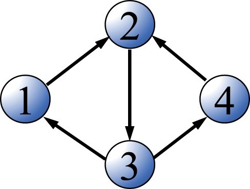
The graph Laplacian of this graph is $\begin{array}{r}L=\left[\begin{array}{cccc}1& 0& -1& 0\\ -1& 2& 0& -1\\ 0& -1& 1& 0\\ 0& 0& -1& 1\end{array}\right].\end{array}$The eigenvalues of L are $\sigma \left(L\right)=\{0,1,2\pm \mathbf{j}\}$, and the left eigenvector corresponding to the zero eigenvalue of L is $\varphi =[0.2,0.2,0.4,0.2{]}^{\mathsf{\text{T}}}$.

We set the parameters for the VE as $\begin{array}{r}S=\left[\begin{array}{cc}0& -0.4\\ 0.4& 0\end{array}\right],R=\left[\begin{array}{cc}0& 1\end{array}\right].\end{array}$This choice means that the synchronization trajectory is generated by the second-order oscillator. Then, the Francis' Equation (9(9) $\begin{array}{rl}{A}_i{\mathrm{\Pi }}_i+B_i{\mathrm{\Gamma }}_i& ={\mathrm{\Pi }}_{i}S\end{array}$(9) )–(10(10) $\begin{array}{rl}{C}_i{\mathrm{\Pi }}_i& =R\end{array}$(10) ) has the following solution. $\begin{array}{rl}{\mathrm{\Pi }}_i& =\left[\begin{array}{cc}1& 0\\ 0& 1\end{array}\right],{\mathrm{\Gamma }}_i=\left[\begin{array}{cc}{a}_i+0.4& -b_i\end{array}\right],i=1,3,\\ {\mathrm{\Pi }}_i& =\left[\begin{array}{cc}0& 1\\ 1& 0\\ 0& -1\end{array}\right],{\mathrm{\Gamma }}_i=\left[\begin{array}{cc}-b_i-0.4& -a_i+1\end{array}\right],\\ & i=2,4.\end{array}$The controller gains $K_i$ and $L_i$ are designed by the pole placement technique so that the eigenvalues of $A_i+B_i{K}_i$ and $A_i+L_i{C}_i$ are assigned at $\{-5,-6\}$ and $\{-3,-4\}$ for i = 1, 3, and $\{-2,-3,-4\}$ and $\{-1,-2,-3\}$ for i = 2, 4.

In order to obtain a suitable gain F, we solve the algebraic Riccati equation $S^{\mathsf{\text{T}}}P+PS-{\varrho }^{-1}PP+I_q=0$with $\varrho =0.6$, and obtain $\begin{array}{r}P=\left[\begin{array}{cc}0.7746& 0\\ 0& 0.7746\end{array}\right].\end{array}$Correspondingly, the feedback gain is obtained by $\begin{array}{r}F=P=\left[\begin{array}{cc}0.7746& 0\\ 0& 0.7746\end{array}\right].\end{array}$We set ${\kappa }_{\theta }=1$, $\theta =0$, $\lambda =0.7736,\kappa =2.3268$, and $s\left(t\right)=0.09+(1-0.09)\exp (-0.3t)$. The parameters of the agents and the corresponding regulator/observer gains are shown in Table 2. The initial estimation error of the observer is set to $[-1,-1{]}^{\mathsf{\text{T}}}$ for i = 1, 3, and $[-1,-1,-1{]}^{\mathsf{\text{T}}}$ for i = 2, 4. The initial local tracking errors are set to ${ϵ}_1\left(0\right)=[1,1{]}^{\mathsf{\text{T}}},{ϵ}_2(0)=[-5.3,11.3,4.3{]}^{\mathsf{\text{T}}},{ϵ}_3\left(0\right)=[2,2{]}^{\mathsf{\text{T}}}$, and ${ϵ}_4\left(0\right)=[-3.9,9.9,8{]}^{\mathsf{\text{T}}}$. The tolerances ${\chi }_i^{\mathrm{o}\mathrm{u}\mathrm{t}},i=1,\dots ,4$ are computed as 0.8513, 0.9666, 1.0550, and 1.2547 by (36(36) $\begin{array}{rl}{\chi }_i^{\mathrm{o}\mathrm{u}\mathrm{t}}& ={\kappa }_{{ϵ}_i}\kappa {\text{β}}_i\sqrt{N}\Vert C_i\Vert \Vert {\mathrm{\Pi }}_i\Vert \Vert {\mathcal{B}}^{\prime }\Vert (\frac{s_{\mathrm{\infty }}}{\lambda }\frac{1}{{\lambda }_{{ϵ}_i}}+\frac{s_{\mathrm{\infty }}}{{\lambda }_{{ϵ}_i}})\\ & +\Vert R\Vert \frac{\kappa \sqrt{N}\Vert {\mathcal{B}}^{\prime }\Vert s_{\mathrm{\infty }}}{\lambda }.\end{array}$(36) ), respectively.

Table 2. Parameters.

i	$(a_i,b_i)$	$(K_i,L_i)$
1	$(-4.5,0.3)$	$\left(\right[25.5,-7.3],\left[\begin{array}{c}-0.94\\ -5.3\end{array}\right])$
2	$(7.9,0.1)$	$\left(\right[-157.9,-65.1,-10.0],\left[\begin{array}{c}-7.0\\ -45.1\\ -159.9\end{array}\right])$
3	$(-1.9,-0.6)$	$\left(\right[28.1,-6.4],\left[\begin{array}{c}-2.76\\ -4.4\end{array}\right])$
4	$(6.3,0.9)$	$\left(\right[-156.3,-65.9,-10.0],\left[\begin{array}{c}-7.0\\ -45.9\\ -174.3\end{array}\right])$

The simulation results are shown in Figures 5–7. We run the simulation in 8 seconds. Figure 5 shows the outputs of the agents, and Figure 6 shows the synchronization error $|y_i-R\alpha |,i=1,\dots ,4$.

We can observe that the outputs of all the agents synchronize as time increases, and the synchronization errors are sufficiently small. The synchronization error $|y_i-R\alpha |$ is less than ${\chi }_i^{\mathrm{o}\mathrm{u}\mathrm{t}}$ within the simulation time for all the agents.

Figure 5. Outputs y.

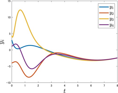
Figure 6. Output synchronization error $|y_i-R\alpha |$.

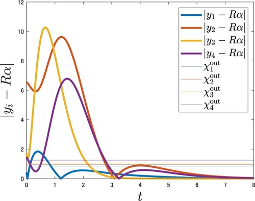
Figure 7. States of the virtual exosystems at access times.

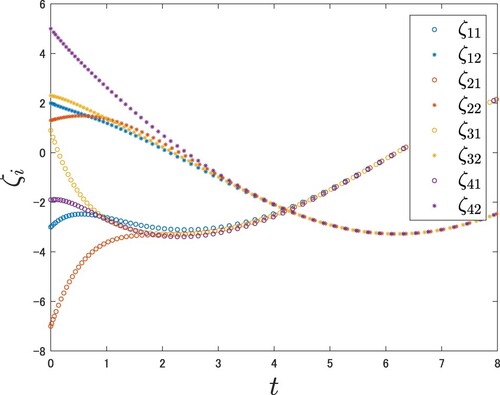
The trajectories of the VEs are shown in Figure 7. We can observe that the trajectories of the VEs are achieving the bounded state synchronization within the tolerance given by (31(31) $\underset{t\to \mathrm{\infty }}{lim}sup\Vert \delta \left(t\right)\Vert \le \frac{\kappa \sqrt{N}\Vert {\mathcal{B}}^{\prime }\Vert s_{\mathrm{\infty }}}{\lambda }$(31) ). It is also seen that any Zeno behaviour does not occur. By using (A5(A5) ${\tau }_i^{\star }=\frac{s_{\mathrm{\infty }}}{{\gamma }_i}>0.$(A5) ) in Appendix A.2, we can compute the theoretical lower bounds of the access intervals ${\tau }_1^{\star }=0.0014$, ${\tau }_2^{\star }=0.0008$, ${\tau }_3^{\star }=0.0015$, and ${\tau }_4^{\star }=0.0011\left[\mathrm{s}\right]$. Actually, the minimum and average access intervals are much larger than the theoretical lower bounds of the access intervals as shown in Table 3.

Table 3. Cloud accesses of virtual exosystems.

	Access	Minimum interval	Average interval
1	64	0.0182	0.1259
2	65	0.0161	0.1247
3	63	0.0303	0.1268
4	63	0.0330	0.1280

5. Concluding remarks

In this paper, we proposed the cloud-mediated output synchronization controller for the heterogeneous linear multi-agent system based on the self-triggered control. The proposed method achieves the bounded output synchronization with asynchronous communication between the cloud repository and the agents. The numerical simulation shows the effectiveness of our method.

As a future work, it may be possible to study the relationship between the proposed method and conventional controller design techniques for time-delay systems.

Acknowledgments

The authors would like to thank anonymous reviewers for their insightful comments.

Disclosure statement

No potential conflict of interest was reported by the author(s).

Correction Statement

This article has been corrected with minor changes. These changes do not impact the academic content of the article.

Additional information

Funding

This work is supported by JST-SPRING JPMJSP2101.

Notes on contributors

Takumi Namba

Takumi Namba received his B.Eng. and M.Eng. from Ritsumeikan University, Japan in 2018 and 2020, respectively. From April 2020 to August 2021, he was with the Grid Aggregation Division, Toshiba Energy and Systems Solutions Corporation, Japan. From September 2021, he is with the Graduate School of Science and Engineering, Ritsumeikan University, and currently working toward his Ph.D. degree. His current research interests include distributed energy management systems based on distributed and cooperative controls. He is a student member of SICE, ISCIE, and IEEE.

Kiyotsugu Takaba

Kiyotsugu Takaba received his B.Eng., M.Eng., and Dr.Eng. degrees all from Kyoto University, Japan, in 1989, 1991, and 1995, respectively. From 1991 to 1998, he was an Assistant Professor at the Department of Applied Mathematics and Physics, Kyoto University. From 1998 to 2012, he was an Associate Professor at the same department. In 2012, he joined the Department of Electrical and Electronic Engineering, Ritsumeikan University, where he is currently a Professor. His current research interests include robust/optimal control, optimal filtering, and cooperative control for multivariable dynamical systems and their applications. He is a member of SICE, ISCIE, IEEE, and SIAM.

Appendix

A.1. Proof of Lemma 3.1

Proof.

By solving (20(20) $\dot{\delta }\left(t\right)=\mathcal{S}\delta \left(t\right)+{\mathcal{B}}^{\prime }\tilde{v}\left(t\right),$(20) ), the time evolution of $\delta \left(t\right)$ from $t_0$ is given by (A1) $\delta \left(t\right)={\mathrm{e}}^{\mathcal{S}(t-t_0)}\delta \left(t_0\right)+{\int }_{t_0}^t{\mathrm{e}}^{\mathcal{S}(t-\tau )}{\mathcal{B}}^{\prime }\tilde{v}\left(\tau \right)\mathrm{d}\tau .$(A1) By a technique similar to Lemma 3.1 in [11], it turns out that, if $\check{\mathcal{S}}$ is Hurwitz stable and $\mathbf{v}$ satisfies $({\varphi }^{\mathsf{\text{T}}}\otimes I_q)\mathbf{v}=0$, there exist $\lambda >0$ and $\kappa >0$ satisfying (28(28) $\Vert {\mathrm{e}}^{\mathcal{S}t}\mathbf{v}\Vert \le \kappa {\mathrm{e}}^{-\lambda t}\Vert \mathbf{v}\Vert ,$(28) ). It should be noted that δ and ${\mathcal{B}}^{\prime }\tilde{v}$ meet the above condition for $\mathbf{v}$.

It then follows that $\Vert \delta \left(t\right)\Vert \le \kappa {\mathrm{e}}^{-\lambda (t-t_0)}\Vert \delta \left(t_0\right)\Vert +{\int }_{t_0}^t\kappa {\mathrm{e}}^{-\lambda (t-\tau )}\Vert {\mathcal{B}}^{\prime }\Vert \Vert \tilde{v}\left(\tau \right)\Vert \mathrm{d}\tau .$By using (22(22) $\Vert {\tilde{v}}_i\left(t\right)\Vert \le s\left(t\right),\mathrm{\forall }i\in \mathcal{V}$(22) ), we further bound $\delta \left(t\right)$ as $\begin{array}{rl}\Vert \delta \left(t\right)\Vert & \le \kappa {\mathrm{e}}^{-\lambda (t-t_0)}\Vert \delta \left(t_0\right)\Vert \\ & +\kappa \sqrt{N}\Vert {\mathcal{B}}^{\prime }\Vert {\int }_{t_0}^t{\mathrm{e}}^{-\lambda (t-\tau )}s\left(\tau \right)\mathrm{d}\tau .\end{array}$Let ${\eta }_0$ be a constant which satisfies ${\eta }_0\ge \Vert \delta \left(t_0\right)\Vert$. Then, by comparing the RHS of the above inequality with (26(26) $\begin{array}{rl}\eta \left(t\right)& :=\kappa {\mathrm{e}}^{-\lambda (t-t_0)}{\eta }_0\\ & +\kappa \sqrt{N}\Vert {\mathcal{B}}^{\prime }\Vert {\int }_{t_0}^t{\mathrm{e}}^{-\lambda (t-\tau )}s\left(\tau \right)\mathrm{d}\tau ,\end{array}$(26) ), we obtain the inequality (24(24) $\begin{array}{rl}& \Vert \delta \left(t\right)\Vert \le \eta \left(t\right),\mathrm{\forall }t\in [t_0,t_f[,\end{array}$(24) ).

It remains to prove the second inequality (25(25) $\begin{array}{rl}& \Vert v_j\left(t\right)\Vert \le {\mu }_j\left(t\right),\mathrm{\forall }j\in \mathcal{V},\mathrm{\forall }t\in [t_0,t_f[,\end{array}$(25) ). Recall that the relative state feedback control law can be expressed as $z_i\left(t\right)=F\sum _{j\in {\mathcal{N}}_i}\left({\delta }_j\right(t)-{\delta }_i(t\left)\right).$Thus, $z_i\left(t\right)$ is represented by (A2) $z_i\left(t\right)=-[L\otimes F{]}_i\delta (t),$(A2) and taking norms of both sides leads to $\Vert z_i\left(t\right)\Vert \le {\text{β}}_i\Vert \delta \left(t\right)\Vert .$Therefore, we obtain (A3) $\Vert v_i\left(t\right)\Vert \le \Vert z_i\left(t\right)\Vert +\Vert {\tilde{v}}_i\left(t\right)\Vert \le {\text{β}}_i\eta \left(t\right)+s\left(t\right).$(A3) Recall from (27(27) $\begin{array}{rl}{\mu }_j\left(t\right)& :={\text{β}}_j\eta \left(t\right)+s\left(t\right),\end{array}$(27) ) that the RHS of (A3(A3) $\Vert v_i\left(t\right)\Vert \le \Vert z_i\left(t\right)\Vert +\Vert {\tilde{v}}_i\left(t\right)\Vert \le {\text{β}}_i\eta \left(t\right)+s\left(t\right).$(A3) ) is equal to ${\mu }_i\left(t\right)$. By replacing the suffix i to j, it concludes the proof.

A.2. Proof of Lemma 3.2

Proof.

We can express the input error $\Vert {\tilde{v}}_i\left(t\right)\Vert$ by $\begin{array}{rl}\Vert {\tilde{v}}_i\left(t\right)\Vert & =\Vert v_i\left(t\right)-F\sum _{j\in {\mathcal{N}}_i}\left({\hat{\zeta }}_j^i\right(t)-{\zeta }_i(t\left)\right)\\ & -F\sum _{j\in {\mathcal{N}}_i^{\prime }\left(t\right)}{\int }_{t_j^{l_j+1}}^t{\mathrm{e}}^{S(t-\tau )}{v}_j\left(\tau \right)\mathrm{d}\tau \Vert .\end{array}$Application of the triangular inequality to the above equation yields (A4) $\begin{array}{rl}\Vert {\tilde{v}}_i\left(t\right)\Vert & \le \Vert v_i-F\sum _{j\in {\mathcal{N}}_i}\left({\hat{\zeta }}_j^i\right(t)-{\zeta }_i(t\left)\right)\Vert \\ & +\Vert F\Vert {\kappa }_{\theta }\sum _{j\in {\mathcal{N}}_i^{\prime }\left(t\right)}{\int }_{t_j^{l_j+1}}^t{\mathrm{e}}^{\theta (t-\tau )}\Vert v_j\left(\tau \right)\Vert \mathrm{d}\tau .\end{array}$(A4) By invoking the contraposition of Lemma 3.1, we can show that $\Vert {\tilde{v}}_i\left(t\right)\Vert \le {\sigma }_i^{l_i}\left(t\right)$ will not be violated unless some of the agents violate the condition. Because the choice $\Vert {\tilde{v}}_i\left(0\right)\Vert =0$ is possible, we can conclude the former statement of Lemma 3.2.

Next, we will prove the Non-Zenoness of the proposed algorithm (for more detail, refer to [17,18]). Firstly, we consider the case of $\theta =0$. By some computations, we can bound ${\sigma }_i^{l_i}\left(t\right)$ in (32(32) $\begin{array}{rl}{\sigma }_i^{l_i}\left(t\right)& :=f_i^{l_i}\left(t\right)+g_i^{l_i}\left(t\right),\end{array}$(32) )–(34(34) $\begin{array}{rl}{g}_i^{l_i}\left(t\right)& :={\kappa }_{\theta }\sum _{j\in {\mathcal{N}}_i^{\prime }\left(t\right)}{\int }_{t_j^{l_j+1}}^t{\mathrm{e}}^{\theta (t-\tau )}{\mu }_j\left(\tau \right)\mathrm{d}\tau ,\end{array}$(34) ) as $\begin{array}{rl}{\sigma }_i^{l_i}\left(t\right)& =f_i^{l_i}\left(t\right)+g_i^{l_i}\left(t\right)\\ & \le {\text{β}}_i\overline{\eta }\Vert S\Vert (t-t_i^{l_i})\\ & +\Vert F\Vert {\kappa }_{\theta }\sum _{j\in {\mathcal{N}}_i}({\text{β}}_j\overline{\eta }+s_0)(t-t_i^{l_i})\\ & +\Vert F\Vert {\kappa }_{\theta }\sum _{j\in {\mathcal{N}}_i}\left\{\right({\text{β}}_i+{\text{β}}_j)\overline{\eta }+2s_0\}(t-t_i^{l_i})\\ & =\Vert F\Vert {\kappa }_{\theta }\sum _{j\in {\mathcal{N}}_i}\left\{\right({\text{β}}_i+2{\text{β}}_j)\overline{\eta }+3s_0\}(t-t_i^{l_i})\\ & +{\kappa }_{\theta }{\text{β}}_i\overline{\eta }\Vert S\Vert (t-t_i^{l_i})\\ & ={\gamma }_i(t-t_i^{l_i}),\end{array}$with ${\gamma }_i=\Vert F\Vert {\kappa }_{\theta }\sum _{j\in {\mathcal{N}}_i}({\text{β}}_i+2{\text{β}}_j)\overline{\eta }+3s_0+{\kappa }_{\theta }{\text{β}}_i\overline{\eta }\Vert S\Vert ,$where $\overline{\eta }$ is an upper bound on $\eta \left(t\right)$. Recall that $s\left(t\right)$ satisfies $s\left(t\right)\ge s_{\mathrm{\infty }},\mathrm{\forall }t\ge t_i^{l_i}$. Thus, the triggering condition ${\sigma }_i^{l_i}\left(t\right)\ge s\left(t\right)$ in (29(29) $t_i^{l_i+1}=inf\{t>t_i^{l_i}|{\sigma }_i^{l_i}(t)\ge s(t\left)\right\}.$(29) ) is not satisfied unless ${\gamma }_i(t-t_i^{l_i})<s_{\mathrm{\infty }},\mathrm{\forall }t\ge t_i^{l_i}$ is violated. Define ${\tau }_i^{\star }$ as the smallest positive root for the following equation. (A5) ${\tau }_i^{\star }=\frac{s_{\mathrm{\infty }}}{{\gamma }_i}>0.$(A5) It should be noted that the triggering condition (29(29) $t_i^{l_i+1}=inf\{t>t_i^{l_i}|{\sigma }_i^{l_i}(t)\ge s(t\left)\right\}.$(29) ) is not satisfied before $t_i^{l_i}+{\tau }_i^{\star }$, and ${\tau }_i^{\star }$ does not depend on $t_i^{l_i}$. Hence, ${\tau }_i^{\star }$ is a lower bound on $t_i^{l_i+1}-t_i^{l_i}$ for the triggering rule (29(29) $t_i^{l_i+1}=inf\{t>t_i^{l_i}|{\sigma }_i^{l_i}(t)\ge s(t\left)\right\}.$(29) ), namely $t_i^{l_i+1}-t_i^{l_i}\ge {\tau }_i^{\star }$, $\mathrm{\forall }i,l_i$.

Similarly, in the case of $\theta \ne 0$, we can bound ${\sigma }_i^{l_i}\left(t\right)$ as (A6) ${\sigma }_i^{l_i}\left(t\right)\le {\gamma }_i\frac{{\mathrm{e}}^{\theta (t-t_i^{l_i})}-1}{\theta }.$(A6) Let ${\tau }_i^{\star }$ be the smallest positive root for the following equation. (A7) ${\gamma }_i\frac{{\mathrm{e}}^{\theta {\tau }_i^{\star }}-1}{\theta }=s_{\mathrm{\infty }}$(A7) In the case of $\theta >0$, ${\tau }_i^{\star }$ is explicitly given by (A8) ${\tau }_i^{\star }=\frac{1}{\theta }\ln (1+\frac{\theta s_{\mathrm{\infty }}}{{\gamma }_i})>0,\mathrm{\forall }i,l_i.$(A8) In the case of $\theta <0$, Equation (A7(A7) ${\gamma }_i\frac{{\mathrm{e}}^{\theta {\tau }_i^{\star }}-1}{\theta }=s_{\mathrm{\infty }}$(A7) ) may not have any root. However, such a case means that the VE dynamics is stable and the desired tolerance is large. It may be noted that, in this case, we can choose the next access time arbitrarily large. Thus, the non-Zenoness is also guaranteed.

We can conclude that the closed-loop system does not exhibit any Zeno behaviour.

References

- Saber R, Fax JA, Murray RM. Consensus and cooperation in networked multi-agent systems. Proc IEEE. 2007;95(1):215–233.
- Scardovi L, Sepulchre R. Synchronization in network of identical linear systems. Automatica. 2009;45(11):2557–2562.
- Li Z, Duan Z, Chen G, et al. Consensus of multiagent systems and synchronization of complex networks: a unified viewpoint. IEEE Trans Circuits Syst I. 2010;57(9):2552–2563.
- Takaba K. Robust synchronization of linear multi-agent system with input/output constraints. Artif Life Robot. 2018;23:577–584.
- Trentelman H, Takaba K, Monshizadeh N. Robust synchronization of uncertain linear multi-agent systems. IEEE Trans Automatic Control. 2013;58(6):1511–1523.
- Nowzari C, Garcia E, Cortés J. Event-triggered communication and control of networked systems for multi-agent consensus. Automatica. 2019;105:1–27.
- Yang D, Ren W, Liu X. Decentralized consensus for linear multi-agent systems under general directed graphs based on event-triggered/self-triggered strategy. Proc 53rd IEEE Conf. on Decision and Control; 2014; p. 1984–1988.
- Dimarogonas DV, Frazzoli E, Johansson KH. Distributed self-triggered control for multi-agent systems. Proc 2010 IEEE 49th Conference on Decision and Control; 2010; p. 6716–6721.
- Ding L, Han QL, Ge X, et al. An overview of recent advances in event-triggered consensus of multiagent systems. IEEE Trans Cybernetics. 2017;48(4):1110–1123.
- Zhu W, Jiang ZP, Feng G. Event-based consensus of multi-agent systems with general linear models. Automatica. 2014;50(2):552–558.
- Almeida J, Silvestre C, Pascoal A. Synchronization of multiagent systems using event-triggered and self-triggered broadcasts. IEEE Trans Automatic Control. 2017;62(9):4741–4746.
- Adaldo A, Liuzza D, Dimarogonas DV, et al. Control of multi-agent systems with event-triggered cloud access. Proc 2015 European Control Conference (ECC); 2015; p. 954–961.
- Adaldo A, Liuzza D, Dimarogonas DV, et al. Multi-agent trajectory tracking with self-triggered cloud access. Proc 2016 IEEE 55th Conference on Decision and Control; 2016; p. 2207–2214.
- Nowzari C, Pappas GJ. Multi-agent coordination with asynchronous cloud access. Proc 2016 American Control Conference; 2016; p. 4649–4654.
- Bowman SL, Nowzari C, Pappas GJ. Consensus of multi-agent systems via asynchronous cloud communication. IEEE Trans Control Netw Syst. 2020;7(2):627–637.
- Adaldo A, Liuzza D, Dimarogonas DV, et al. Cloud-supported formation control of second-order multi-agent systems. IEEE Trans Control Netw Syst. 2017;5(4):1563–1574.
- Namba T, Takaba K. Self-triggered synchronization of a linear multi-agent system through a cloud repository. IFAC-PapersOnLine. 2022;55(13):157–161.
- Namba T, Takaba K. Cloud-mediated self-triggered synchronization of a general LTI multi-agent system over a directed graph. submitted for publication; 2022.
- Namba T, Takaba K. Cloud-mediated self-triggered synchronization of linear agents subject to disturbances. IFAC World Congress 2023; 2023; (to appear).
- Hong S, Zhang Y. Cloud-based self-triggered coordination for nonlinear multi-agent consensus. Neurocomputing. 2023;520:171–182.
- Wieland P, Allgöwer F. An internal model principle for consensus in heterogeneous linear multi-agent systems. IFAC Proc. 2009;42(20):7–12.
- Wieland P, Sepulchre R, Allgöwer F. An internal model principle is necessary and sufficient for linear output synchronization. Automatica. 2011;47(5):1068–1074.
- Hu W, Liu L, Feng G. Output consensus of heterogeneous linear multi-agent systems by distributed event-triggered/self-triggered strategy. IEEE Trans Cybern. 2016;47(8):1914–1924.
- Almeida J, Silvestre C, Pascoal AM. Output synchronization of heterogenous LTI plants with event-triggered communication. Proc 53rd IEEE Conf. on Decision and Control; 2014; p. 3572–3577.
- Bullo F. Lectures on network systems. Kindle Direct Publishing; 2022. Edition 1.6.
- Francis BA, Wonham WM. The internal model principle for linear multivariable regulators. Appl Math Optim. 1975;2(2):170–194.
- Knobloch HW, Isidori A, Flockerzi D. Topics in control theory. Basel: DMV seminar. Bd. 22. Birkhäuser Verlag; 1993.
- Zhang H, Lewis FL, Das A. Optimal design for synchronization of cooperative systems: state feedback, observer, and output feedback. IEEE Trans Automat Control. 2011;56(8):1948–1952.