Dynamic life cycle costing based on lifetime prediction

Abstract

Reliable prediction of total product life cycle costs is crucial for the life cycle management of products. These costs are predominantly dictated by the actual operational behaviour of the product's lifetime, and cannot be sufficiently determined through deterministic calculations due to the stochastic and the dynamic nature of the problem. This is specifically true when considering running systems with unknown lifetime and operation parameters. Against this background, the paper presents a dynamic methodology for predicting life cycle costs based on product failure mechanisms, their associated critical lifetime prediction parameters and optional maintenance strategies to enable decision support for product design and use phase strategies.

Keywords:

• life cycle
• life cycle costing
• LCC
• maintenance

Introduction

Life cycle costing (LCC) is a major concern to foster a successful product life cycle management (Herrmann et al. 2007a). LCC allows the identification of main cost drivers while considering all economically relevant monetary flows over the whole life cycle. Hence, with this holistic perspective, LCC enables the derivation of promising measures to influence these costs (e.g. decision support for product design phase) while avoiding unfavourable problem shifting through life cycle phases.

For the calculation of life cycle costs, different concepts have been developed which differ with respect to their scope (e.g. life cycle phase, manufacturer or operator costs and yield), transferability to different fields of application, definition of cost portions/life cycle phases or the treatment of financial aspects (e.g. discounting) (IEC 2004, VDI 2005, VDMA 2006, Frank et al. 2007). Total cost of ownership (TCO) is one of these concepts while considering all operator-related costs.

Diverse studies for technical products underline that major cost shares actually occur during the later stages of the product life cycle, e.g. energy and maintenance costs during the use phase (e.g. studies on industrial pumps, military equipment, e.g. Komarek 2001). As an example, Figure 1 exemplarily shows a TCO analysis for an electric drive.

Figure 1 Life cycle costs of electric drive system (operator view) (data based on Bockskopf 2007).

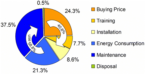
While the two cost factors energy and maintenance are typically most important, their predictability is very restrained. In contrast to the other static or quasi-static cost variables such as the acquisition price or certain cost amounts for ramp-up (e.g. training, installation) or disposal, the costs within the use phase are highly dynamic depending on the actual states of the machine or its components. These states depend on complex influence variables such as the actual usage profile and certain environmental conditions. Specifically, the maintenance costs can be highly influenced through the selection of maintenance strategies. As a result, including strategies and their effects is crucial when estimating maintenance costs that are an integral part of life cycle cost calculation. Additionally, choosing the right strategy for maintaining a machine over its whole lifetime can be seen as a major task for companies to achieve economically optimal solutions (e.g. Takata et al. 2004, Feldman et al. 2009).

Technical background

Maintenance

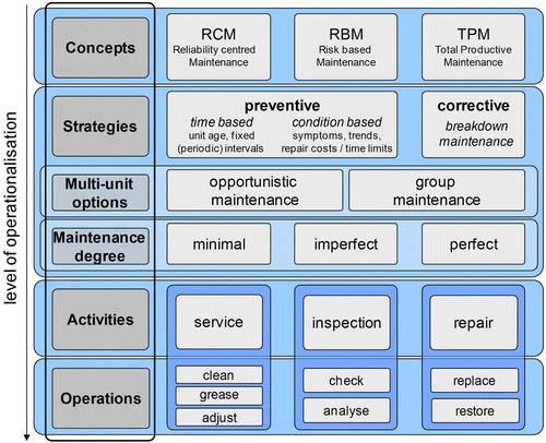
Maintenance has naturally been a very important topic in research for years; besides, many basic standards and literature about certain configuration alternatives, there are also studies and calculation models trying to derive optimal strategies under certain circumstances. While there is a diversity of expressions (sometimes used in different contexts and hierarchical orders), Figure 2 shows a hierarchical framework of maintenance terminology, which idealistically displays maintenance alternatives (Herrmann et al. 2007b based on Takata et al. 2004, Wang 2002, DIN 2003) as a base for this paper. Basically, four major layers can be differentiated which lead from actual operations/actions (e.g. cleaning, replacing) and activities that are being combined to certain strategies (preventive, corrective) and embedded within holistic concepts (e.g. reliability centred maintenance (RCM), risk based maintenance (RBM), total productive maintenance (TPM) (Herrmann et al. 2007b).

Figure 2 Hierarchical framework of maintenance terminology (Herrmann et al. 2007b based on Wang 2002, DIN 2003, Takata et al. 2004).

A general recommendation regarding an ideal maintenance strategy for a technical system and its components is not possible and not trivially determinable while it depends on every specific case with its diverse influencing variables. Essential factors are the specific progressive pattern of functional degradation under affecting stresses and strains and resulting failure behaviour as well as the serviceability of the product (Takata et al. 2004). Additionally, economic variables such as cost rates for failures/planned stoppage or maintenance personnel and material play a deciding role. Uncertainty is a major issue in this context; due to the dynamic and stochastic nature of the problem, the actual success of a chosen strategy is normally not predictable in advance. While being at least easier for new (unused) products (e.g. based on historic data of comparable systems), this is even more true for running systems with unknown lifetime and previous operation conditions.

Life cycle cost calculation

Although simple LCC calculations can be made manually or with common office software, there are various software applications available to support more complex LCC calculations. There are basically two approaches available to calculate life cycle costs which could also be used in combination. These are:

•	(ex-post) analysis: calculation of costs over life cycle through gathering of actual data and structured cost breakdown structures and
•	(ex-ante) estimation: static or dynamic estimation of costs through cost rates and an assumed behaviour over life cycle, often based on technical parameters such as lifetime or mean time between failure (Kawauchi and Rausand 1999).

Although an ex-post analysis can certainly be an important and a reliable source of improvement ideas for products and processes, it can obviously not be used without historic data. If data are not available (e.g. innovative products/processes, purchasing decisions), then estimation is necessary. As mentioned above, two major cost portions, maintenance and energy costs, are naturally neither static nor easily quantifiable (such as the buying price or specific quite known costs for disposal), but rather highly dynamic and depend on the actual use pattern and on the failure behaviour of a system and its components.

As a consequence, static calculations, even though they are easy to use (Kawauchi and Rausand 1999), cannot be used to estimate the product life cycle costs meaningfully. Naturally, these approaches rely on assuming one behaviour and the associated measures over lifetime. As a result, they conflict with the needs of today's manufacturing environment as they can hardly offer ex-ante decision support from an operator's perspective on a realistic base (Herrmann et al. 2007b).

Against this background, there are also several research approaches which use dynamic methods to predict costs over life cycles of technical systems. In combination with certain cost models and the integration of maintenance impacts, Monte Carlo simulation was used in different contexts already. Examples are the determination of guaranteed TCO of machine tools as base for TCO contracts in the automotive industry or warranty strategies (Fleischer et al. 2007, Kleyner and Sandborn 2008), the derivation of optimal life cycle maintenance strategies in combination with reuse (e.g. Momiyama and Takata 2010) or the calculation of life cycle costs of using prognostic health management (e.g. Scanff et al. 2007, Feldman et al. 2009).

Proposed methodology

Against the described, background the objective of the proposed methodology is the dynamic calculation of life cycle costs, which should realistically address the issues of maintenance and uncertainty within multicomponent technical systems. The methodology aims at application not only in design, but also during use phase (e.g. selection of proper maintenance strategies for running systems). While the knowledge of the actual lifetime of components in running systems is an important factor for deriving promising use phase strategies, the methodology also involves a lifetime prediction concept based on technical parameters.

Dynamic life cycle costing (DLCC)

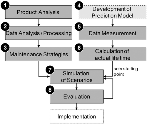
The proposed methodology, as shown in the upper part of Figure 3, has five major phases that are systematically executed in order to integrate dynamic cost portions within life cycle cost calculation as well as to address different maintenance strategies (Herrmann et al. 2007b). These phases are product analysis, data integration and mathematical modelling, integration of maintenance strategies, simulation and evaluation.

Figure 3 Concept of DLCC based on lifetime prediction (Kara et al. 2005, Herrmann et al. 2007b).

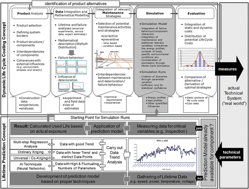
Firstly, an extensive analysis of the considered product is carried out (which, in this case, is a technical system with interacting components) using common methods such as failure mode and effects analysis or Markov Chains (Bertsche and Lechner 2004). This provides system understanding and reveals all relevant components and their internal and external interdependencies. While failure behaviour of components may be quite diverse (stochastic, wear out, instant mortality), it is necessary to get an understanding and mathematical description of failure behaviour which can be described through the progression of the failure rate λ(t) over time. The failure rate curve λ(t) can be derived from empirical data, service statistics or expert estimates. Through mathematical/statistical methods such as the Median rank regression or maximum likelihood method, these data can then be transformed into the necessary input parameters β (it is a shape parameter that describes the mode of failure) and T (it is a scale parameter, the lifetime at which 63.2% of considered units fail) for the Weibull distribution (Equation (1)) which is widely used for these cases because of its flexibility (Abernethy 1993, Bertsche and Lechner 2004, Birolini 2004).

Although there is a broad range of maintenance strategies, corrective and preventive strategies can be basically distinguished to influence the failure behaviour of a system and its components over the lifetime (DIN 2003, Wang 2002, Takata et al. 2004, Herrmann et al. 2007b). In the next step, it is necessary to identify the maintenance activities that are actually relevant to the specific case, e.g. is restoring relevant or an exchange necessary? In order to address the uncertainties associated with the use phase, a simulation model based on Monte Carlo simulation (VDI 1999) is applied. While considering individual component failure rates and system interdependencies as well as other properties such as energy consumption, the effects of certain maintenance strategies, the states of components and system are dynamically calculated and connected with a predetermined cost rate for planned and unplanned maintenance, opportunity costs and energy costs. Using parameter variation, certain scenarios can then be simulated. Due to the stochastic nature of the problem, a sufficient number of simulation runs is essential in order to gain reliable results (Moßig 1996). Finally, static portions of life cycle costs like the purchase price are integrated with the cumulated cost blocks of the simulation runs. As a logical outcome of stochastic analysis and a sufficient amount of simulation runs, there is no single static final result but rather a distribution of values (Fleischer et al. 2007). Important key variables such as cost average, median or occurrence probability of specific quantities can be derived with certain confidence level using the simulation outcome. In addition, costs can also be analysed with respect to their time-based occurrence, and therefore, appropriate financial treatment including interest rates (e.g. discounting – net present value method) can be selected.

Lifetime prediction

Originally, starting from the idea of assessing the remaining lifetime and therefore the reuse potential of components, a methodology for lifetime prediction was developed (Kara et al. 2005, Mazhar 2006). Thereby, the remaining lifetime is the difference between the maximum lifetime of a product and the actual lifetime. This approach also uses the Weibull analysis to predict the maximum lifetime of a product in the first step. The calculation of actual lifetime is based on the verified assumption that the progression of selected explanatory technical parameters is changing over the lifetime of a product (e.g. through deterioration). Hence, it is possible to calculate the actual lifetime based on a one-time measurement of these (technical) variables with an appropriate model to describe the coherences between parameters and lifetime (Figure 3). The prediction model has to be developed specifically for each type of component/product in a multistep approach (Figure 3) (Kara et al. 2005, Mazhar 2006) as follows:

Figure 4 Progression of technical variables over lifetime (Mazhar 2006).

Figure 5 Validation of estimation model through R ² analysis (Mazhar 2006).

1.	Firstly, lifetime data have to be gathered experimentally, which means the measurement of the progression of technical variables over the lifetime of the product/component should be carried out. For the case of an electric drive as a typical parameter, the progression of motor speed, temperature, power consumption, voltage or vibrations/frequencies could be measured (Vass et al. 2008). As shown in Figure 4, these values are not constant over time, but show some characteristic behaviour.
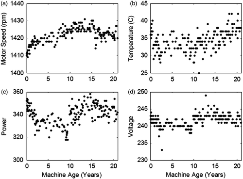2.	Detailed investigations revealed that the suitability of different methods to predict the actual lifetime heavily depends on the progression of measured data (Mazhar 2006). Therefore, a data trend analysis is conducted in order to identify an appropriate technique for lifetime prediction. Thereby, multistep regression analysis, ordinary kriging, universal/co-kriging and artificial neural networks (ANN, artificial intelligence (AI)) are chosen as suitable techniques (Kara et al. 2005). All techniques use (one or several) explanatory variables to calculate the actual lifetime of a component.
3.	Based on the most promising prediction technique, the model is developed (e.g. identification of explanatory variables, training of model) and validated in an iterative process. The quality of prediction is being evaluated through comparing predicted with actual lifetime through using R 2 (coefficient of determination) as an evaluation scale (Mazhar 2006). Figure 5 shows an example for the validation of an ANN prediction model, which underlines the possibility for predicting the actual lifetime with this methodology with an acceptable accuracy.

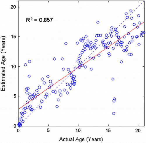The developed methodology has proven to be appropriate to calculate the actual lifetime of a product. Once a prediction model is developed, a one-time measurement of key parameters is sufficient for the estimation. This allows a broad applicability, whereas operating data are often not recorded continuously. As an additional advantage, the actual conditions of use are also considered implicitly in the estimation. For instance, more intensive usage would accelerate the deterioration process and affect the measured technical parameters directly. Thus, the predicted ‘actual’ age is also directly influenced and may result in a value which is, due to actually occurred strain, even higher than the age referring to operating hours.

Integrated approach

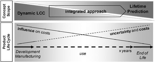
Figure 6 shows an idealistic depiction of the life cycle of technical products. Typically, the use phase is significantly longer compared to other phases and, as described above, a major share of costs occurs here. The life cycle costs are mainly determined with the product design (e.g. dimensioning regarding reliability and maintainability, energy consumption). However, there is also a significant influence on costs in the use phase depending on the use pattern and the actual execution of maintenance measures. This influence on total life cycle costs gets relatively lower over the lifetime. As a third relevant dimension besides costs occurrence and influence, uncertainties related to use phase have to be considered. These uncertainties are stresses and strains, actual operating times, unforeseen internal and external influences or interdependencies (e.g. technology changes, significant changes of cost for labour and/or energy) and stochastic effects (e.g. failures that lead to an unclear time span of usage at all and increasing uncertainty over time). Due to these uncertainties, reliable predictions of cost as well as the derivation of promising measures (e.g. product design) are very difficult at the early stages of the product life cycle.

Figure 6 Classification of addressed approaches in product life cycle.

Figure 6 also illustrates the scopes of the approaches as presented above:

•

Dynamic life cycle costing (DLCC) offers actual decision support on a realistic base during the highly cost relevant system design and use phase. However, the accuracy of the methodology goes down as the time progresses due to the uncertainties related to operating conditions. DLCC originally calculates systems with new and equally aged components and so focuses on early stages of the life cycle. The individual actual lifetime (operating time) of a component is not considered yet, while it is also often not really known in industrial practice. This leads to restricted usability in later stages of the use phase due to the significantly different basic conditions related to the actual use times.

•

As described above, the proposed methodology regarding lifetime prediction was originally intended to evaluate the reuse potential of components in the end of life phase, where not only the problem of the uncertainty in use phase, but also the influence on costs is obviously already restricted. However, the prediction of the actual lifetime without the need of continuous and therefore costly data recording is also useful for the use phase to derive advantageous measures for improvement. As a prerequisite for a successful application, a connection to an evaluation (cost) model including an appropriate method for coping with uncertainty is needed.

The proposed methodology is shown in Figure 7, which integrates the DLCC and the lifetime prediction methods, hence offers a promising approach to derive cost efficient measures for the use phase on a realistic base. The proposed methodology predicts the actual usage life of a product using the measured lifetime prediction parameters. This, in return, can be used as a starting point for the DLCC simulation. The costs are always calculated into the future for the time span considered – starting from the time of the analysis, while costs that occurred in the past are normally not known and also not relevant for the purpose of analysis. The evaluation and comparison of scenarios finally allow the derivation of strategies regarding maintenance or changes in system/product design (e.g. replacing of component with more energy efficient alternative, general modifications of systems).

Figure 7 Process steps for the integrated approach.

Another advantage of this approach is that continuous measurement of system parameters, e.g. operating time, component condition is not necessary, as one-time measurement of relevant parameters enables to derive necessary actions. Considering systems with components which are already in operation for a certain (but unknown) time, the integrated approach calculates the actual life of used components, hence overcoming the previous shortcomings of DLCC, which in return may lead to quite different results at the end. Furthermore, the intensity of usage is also taken into account, which may have a significant impact on the model outcome.

In the end, the proposed methodology leads to more realistic and reliable outcome, which helps to realistically weigh chances and risks of different use phase strategies for the user. The proposed approach goes beyond improving maintenance like other available models for evaluating optimal maintenance strategies, and also enables the evaluation of system modifications by considering all cost components of LCC.

Application

The aforementioned integrated methodology is applied in a case study to demonstrate the feasibility and the potential of the concept. The following steps describe the application as shown in Figures 3 and 7, respectively.

Product and data analysis (1/2)

The considered technical system is located within the main production line of an automobile manufacturer and contains four electric drives of similar type (background data provided in Table 1). Thus, unplanned failures lead to enormous opportunity costs while the whole line/production flow is significantly affected. The electric drives are serially linked – a failure of one component directly leads to a failure of the whole system. The Weibull analysis based on failure data was conducted, which resulted in the necessary parameters β and T ( = MTTF) for the Weibull equation as description of the basic failure behaviour (Kara et al. 2005, Mazhar 2006) (Table 1).

Table 1 Data set for the case study (based on Kara et al. 2005).

	MTTF (years)	Shape parameter (β)	Power consumption (kW)	MTTR (h)
Electric motor (E1)	42.3	4.973	0.4	0.5
Electric motor (E2)	42.3	4.973	0.4	0.5
Electric motor (E3)	42.3	4.973	0.4	0.5
Electric motor (E4)	42.3	4.973	0.4	0.5
Time span				20 years
Maintenance personnel cost rate				60 €/h
Downtime costs (unplanned, e.g. failures)				60.000 €/h
Downtime costs (planned)				0 €/h
Disposal costs				0 €/h
Energy cost rate				0.11 €/kWh
Price per component				1.000 €

Maintenance strategies (3)

In this step, there are no technical restrictions regarding certain maintenance strategies – all possibilities (Herrmann et al. 2007b) can basically be used.

•	Breakdown maintenance: change of electric drive only in case of failure.
•	Breakdown maintenance plus opportunistic strategy: while not working because of the failure of one component, the other drives are getting inspected and changed if also in critical condition.
•	Periodic maintenance (PM): preventive (time based) maintenance – strict change of component in given intervals of 2, 5 or 10 operating years (PM2, PM5 and PM10).
•	Inspection (I): preventive (condition based) maintenance – inspection of components in given intervals of 2, 5 or 10 operating years and exchange if in critical condition (I2, I5 and I10).

In this case, the maintenance worker does not know the actual lifetime or the condition of each electric drive. Hence, in the maintenance situation, the following operative decisions have to be made:

•	Is an immediate exchange of an electric drive necessary? If yes, how many and which electric drive(s) should be replaced?
•	Which is the most favourable maintenance strategy from a cost perspective that should be applied for the next years?

It is obvious that both questions strongly depend on each other and an ideal solution is not trivial to find. It underlines the traditional dilemma of maintenance of balancing high availability (avoiding risk of significant failures costs) and ongoing effort for spare parts and labour. In the following section, specific maintenance activities are abbreviated with the numbers of drives exchanged immediately in the order of predicted actual lifetime (Cx) combined with the maintenance strategy (e.g. I5 for inspection every five years) – e.g. C2I5 stands for an immediate exchange of the two oldest drives and an inspection strategy with 5-year interval.

Prediction model, data measuring, calculation of actual lifetime (4–6)

For the specified electric drives, multiple regression model is used for predicting the remaining life (Kara et al. 2005, Mazhar 2006). For this purpose, the following Equation (2) is employed (Kara et al. 2005):

As a result, the prediction results in an R ² (coefficient of determination) of 0.8232, which is deemed acceptable for practical applications (Kara et al. 2005). Certain technical parameters were measured in order to calculate the actual lifetime L _A (Table 2), since the actual operating time of each electric drive is unknown.

Table 2 Measured conditions of use and calculated actual lifetime.

	Component
Parameter	Motor 1	Motor 2	Motor 3	Motor 4
Speed (ω)	1424	1420	1431	1418
Power (P)	343	352	351	350
Temperature (T)	28	40	38	34
Voltage (V)	240	240	245	242
Current (I)	1.75	1.75	1.75	1.75
Calculated actual lifetime (L A)	12.45	9.87	18.15	7.85

Simulation of scenarios and evaluation (7/8)

The results of the Weibull analysis and actual lifetime calculation serve as input data for Monte Carlo simulation to calculate the TCO (relevant cost portions are here: energy costs, direct maintenance costs through personnel and spare parts, opportunity costs for unplanned stops through failures and acquisition costs) for each relevant maintenance strategy. The simulation model run is 385 per considered scenario in order to achieve a confidence interval of 95% with an error ϵ of 0.05.

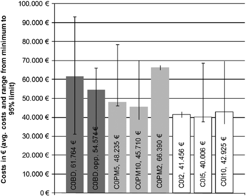
Firstly, a simulation analysis of maintenance strategies was conducted assuming that no drive is exchanged immediately (Figure 8). Thereby, the height of the column displays the average total costs of ownership for 20 years out of the 385 simulation runs. Additionally, the range of values is also indicated. The lower boundary depicts the absolute minimum value, whereas the upper boundary subsumes 95% of all values – that means 95% of the calculated final life cycle costs are below this value or, vice versa, just 5% are over it. This is an important perspective while excluding stochastic outliers, which can be interpreted as the statistical certainty to stay below a certain cost limit and is therefore a possible variable to evaluate alternatives under uncertain circumstances.

Figure 8 Simulation results for different maintenance strategies (without drive change).

The first results underline the significant differences in average and the range of life cycle costs depending on the selected maintenance strategy. The results depict the dilemma of maintenance of avoiding possible expensive unplanned stops through certain preventive effort. Breakdown maintenance can result in both the lowest and highest costs depending on the specific case – it involves a wide range of possible costs with a high degree of uncertainty. Preventive measures can decrease this uncertainty and the probability of unplanned stops for the price of high ongoing effort and less exploited components – hence, the determination of appropriate intervals is critical. For further analyses, the following three strategies are selected:

•	The inspection strategy with 5-year interval while it has the lowest average costs.
•	The PM with 10-year interval while it has the lowest average costs of all considered PM strategies.
•	The breakdown maintenance strategy as interesting reference case while it stands for just doing nothing – however, it may lead to the lowest cost at all (lowest minimum value).

Reflecting the actual decision situation for the maintenance worker in this case, the coherences between immediate action and preferable long-term maintenance strategy were investigated (Figures 9 and 10).

Figure 9 Detailed analysis of consequences of maintenance actions on failure probability and costs over lifetime.

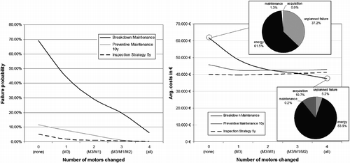
Figure 10 Simulation results of selected maintenance strategies depending on the number of immediately exchanged drives.

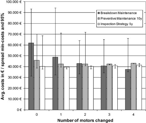
As intuitively expected, there are very strong interdependencies. An exchange of one or more of the oldest drives significantly influences the failure probability of the system. Opportunity costs are quite relevant in this instance, which directly influences the composition of costs and the favourability of different strategies (Figure 9, right-hand side). For example, while being the worst solution in case of no immediate drive exchange, just considering average costs breakdown maintenance is a favourable strategy when replacing three or more drives. However, there is still more risk involved compared to other alternatives.

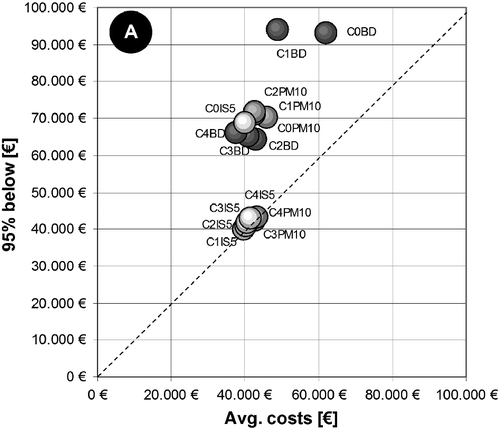
For an integrated evaluation of these complex coherences and the derivation of an appropriate solution, all alternatives were depicted in one diagram considering the critical variables (Figure 11, case A):

Figure 11 Integrated evaluation of alternatives with 95% certainty limit.

•	The average costs over all simulation runs as general and certainly most important criterion regarding the favourability of different strategies.
•	The cost boundary which subsumes 95% of final life cycle cost values over all simulation runs as measure for unfavourable risk and cost spread. Practically speaking – with a certainty of 95% the costs will be below this limit.

Both values shall be as low as possible. In a good case there is no uncertainty and therefore no risk – the value of the y-axis matches the average costs (x-axis) then (however, statistically it is also possible that the y-axis value is lower than the x-axis value). Hence, the objective is to move down in the direction of the dashed line in the diagram as far as possible.

As a result, some general recommendations can be derived by taking this into account. Breakdown maintenance is never a good choice under these circumstances while incorporating too much uncertainty. Additionally, it can be recommended that at least the oldest drive should be replaced while leading to better results in all scenarios. If the exchange of one or more drive is considered, then the inspection strategy is always a good choice. C1IS5 – the exchange of one motor combined with inspections every 5 years – can be identified as the best maintenance strategy for case A with a statistical certainty of 95% and costs approximately over 40.000€ over 20 years.

However, preventive measures like inspections imply certain effort that may not be necessary, as reducing risk can cost a significant amount of money. Therefore, from a user's perspective, it is certainly a possible objective to save on costs occurring for ongoing preventive measures while accepting a slightly higher risk of failures that may lead to slight cost increase. These thoughts are reflected in case B (Figure 12). Based on the same scenarios and simulation results, the limit regarding statistical certainty was decreased to 90% – meaning that with a probability of 10%, the costs may be higher than the indicated value due to unforeseen failures.

Figure 12 Integrated evaluation of alternatives with 90% certainty limit (B) and detailed view also considered alternative type of electric drive (C).

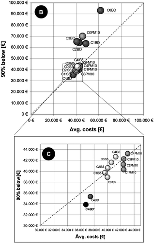
These circumstances lead to different results of the evaluation. It is now most favourable to replace all four drives immediately while accepting a certain risk and to follow a breakdown maintenance strategy with low running costs afterwards (the risk of failures of new electric drives is naturally significantly lower). On average, this results in cost savings of over 10% over 20 years (see detailed illustration in Figure 12).

As already shown in Figure 9, the share of maintenance costs on TCO can be significantly decreased through improved maintenance measures while energy costs even more dominate. Energy consumption is certainly the main leverage for further improvement of total costs. Therefore, the proposed methodology can also provide decision support in this context due to the broad focus on all relevant components of life cycle costs. One promising approach might be the usage of more energy efficient electric drives [called class EFF1 referring to the international norm (IEC 2007)] instead of EFF2-drives. EFF1-drives typically offer an efficiency increased by 5% with a price increase of approximately 25% compared to EFF2-drives (e.g. Hanitsch 2002). By taking these numbers (and same data regarding lifetime, etc.) into account, case C in Figure 12 considers the consequent usage of EFF1-drives for the promising strategy C4BD. The results indicate that all four EFF2-drives are replaced by EFF1-drives immediately (C4BD*). The results also reveal that this is actually advantageous to do so, since higher cost for acquisition is more than trade off over 20 years of usage and leads to cost savings over lifetime.

Discussion and conclusion

The case study presented in this paper shows the underlying thinking and the potentials of the integrated methodology. However, the case presented here is relatively a simple example for application on a system with identical components. More complex systems with diverse components and aspects such as additional or changing cost rates (e.g. disposal costs, change of energy prices over time) significantly increase the difficulty of finding cost optimal solutions. In addition, a selection of possible maintenance strategies was considered for the purpose of demonstration. The results indicate that, while the whole complexity is not manually solvable, the proposed approach is able to provide important decision support. In order to address this, it is certainly necessary to convert the underlying logic to a usable software or hardware application.

In comparison to ex-post calculation or static estimation models, this approach offers ex-ante decision support on a realistic base. Thereby, the integration of DLCC and lifetime prediction is a useful contribution. The proposed concept supports for deriving optimal measures regarding maintenance and alternative system design (e.g. component selection) for new and operating systems under consideration of uncertainties in the use phase, which only requires a one-time measurement of technical parameters to predict the actual lifetime The case study underlines that just using the DLCC approach (which assumes a new system – in the case study reflected by replacing all drives in the beginning) neglects realistic circumstances for running systems and may not lead to the best solution. For example, breakdown maintenance would have come out of an isolated DLCC analysis as the best strategy – for the given case, this would be one of the worst alternatives when not considering a total system makeover at the beginning.

From the technological perspective on the product, the proposed methodology allows the funded comparison of alternatives and can be used by operators for evaluating maintenance strategies or changes in system design. Naturally, it is also useful for the developers of products or services. As the case study shows, it thereby allows the conscious consideration of uncertainty/risk as one important decision variable. This leads also to interesting applications in marketing/sales (e.g. TCO-contracts, guarantees).

References

- Abernethy , R.B. 1993 . The new Weibull handbook , Houston : Gulf Publishing Co., ISBN 0-9653062-3-2 .
- Bertsche , B. and Lechner , G. 2004 . Zuverlässigkeit im Fahrzeug- und Maschinenbau , Berlin : Springer .
- Birolini , A. 2004 . Reliability engineering – theory and practice , Berlin : Springer .
- Bockskopf , V. 2007 . Lebenszykluskosten: Genau hinsehen und Kosten sparen . Konstruktion Special Antriebstechnik , S1/2007 : 16 – 18 .
- Deutsches Institut für Normung e.V., 2003. DIN 31051 – Fundamentals of maintenance
- Feldman , K. , Jazouli , T. and Sandborn , P. 2009 . A methodology for determining the return on investment associated with prognostics and health management . IEEE Transactions on Reliability , 58 ( 2 ) : 305 – 316 .
- Fleischer , J. , Wawerla , M. and Niggeschmidt , S. 2007 . “ Machine life cycle cost estimation via Monte-Carlo simulation ” . In Proceedings of the 14th CIRP conference on life cycle engineering 2007 , 449 – 453 . London : Springer . Tokyo, May 2007
- Frank , T. , Niemann , J. and Westkämper , E. 2007 . Ein Tool zur lebenslangen Kostenüberwachung. Vom life cycle costing zum life cycle controlling . wt Werkstatttechnik , 97 ( 7/8 ) : 555 – 559 .
- Hanitsch , R. 2002 . “ Energieeffiziente Antriebe – ein Aspekt beim Energiemanagement ” . In Dokumentation der Fachtagung – Fortschritte in der Energieeffizienz – Potenziale und Umsetzung 4 December, Berlin
- Herrmann , C. 2007a . “ Total life cycle management – an integrated approach towards sustainability ” . In 3rd International conference on life cycle management Zurich, 27–29 August 2007
- Herrmann , C. 2007b . “ Framework for the dynamic and life cycle oriented evaluation of maintenance strategies ” . In Proceedings of 3rd international VIDA conference, Poznan , 277 – 284 . Poznan : Publishing House of Poznan University of Technology . June 2007
- International Electrotechnical Commission (IEC), 2004. IEC 60300-3-3:2004(E) – Application guide – life cycle costing. CENELEC (European Committee for Electronical Standardization), Brussels
- International Electrotechnical Commission (IEC), 2007. EN 60034-2-1 – Rotating electrical machines – Part 2-1: Standard methods for determining losses and efficiency from tests (excluding machines for traction vehicles), September 2007
- Kara , S. 2005 . Determining the reuse potential of components based on life cycle data . CIRP Annals , 54 ( 1 ) : 1 – 4 .
- Kawauchi , Y. and Rausand , M. 1999 . Life cycle cost (LCC) analysis in oil and chemical process industries , Chiba : Toyo Engineering Corp .
- Kleyner , A. and Sandborn , P. 2008 . Minimizing life cycle cost by managing product reliability via validation plan and warranty return cost . International Journal of Production Economics , 112 ( 2 ) : 796 – 807 .
- Komarek , J. 2001 . “ Life cycle cost simulation in defence planning ” . In RTO SAS symposium on ‘Cost structure and life cycle cost (LCC) for military systems’ Paris, France, 24–25 October 2001
- Mazhar, M., 2006. Lifetime monitoring of appliances for reuse. Thesis (PhD). University of New South Wales
- Momiyama , T. and Takata , S. 2010 . “ Life cycle maintenance in combination with reuse – application to valve actuators for reducing life cycle cost and environmental load ” . In Proceedings of the 17th CIRP conference on life cycle engineering 2010 Hefei, China
- Moßig , I. 1996 . Stichproben, Stichproben-Auswahlverfahren und Berechnung des minimal erforderlichen Stichprobenumfangs unpublished manuscript, Department of geography, Justus-Liebig-Universität Gießen
- Scanff , E. 2007 . Life cycle cost impact of using prognostic health management (PHM) for helicopter avionics . Microelectronics Reliability , 47 ( 12 ) : 1857 – 1864 .
- Takata , S. 2004 . Maintenance: changing role in life cycle management . Annals of the CIRP , 53 ( 2 ) : 1 – 13 .
- Vass , J. 2008 . “ Vibration-based approach to lifetime prediction of washing machines ” . In Proceedings of the 15th CIRP conference on life cycle engineering 2008 Sydney, 17–19 March 2008
- Verein deutscher Ingenieure (VDI) . 1999 . VDI-Guideline 4008 – Monte-Carlo-Simulation , Berlin : Beuth . Blatt 6
- Verein deutscher Ingenieure (VDI) . 2005 . VDI-Guideline 2884 – Purchase, operating and maintenance of production equipment using life cycle costing (LCC) , Berlin : Beuth .
- Verband Deutscher Maschinen-und Anlagenbau e.V. (VDMA) . 2006 . VDMA – Einheitsblatt 34160 (Entwurf) – Prognosemodell für die Lebenszykluskosten von Maschinen und Anlagen , Berlin : Beuth .
- Wang , H. 2002 . A survey of maintenance policies of deteriorating systems . European Journal of Operational Research , 139 : 469 – 489 .