Decision rules for recycling returned products

Abstract

Most retail and on-line outlets allow customers to easily return defective or even non-defective products. Due to increasing environmental and sustainable concerns, disposal of returned products is often costly and undesirable. Furthermore, these products contain parts and materials of value that can contribute to the companies' profit. One way to take advantage of these returns is by utilising good returned parts in production of after-market products. Recycling of parts from products at the end of their useful lives has been studied for a long time. Many of these studies, however, are focused on repairs and refurbishing of such products for reuse.

This paper addresses recycling of rather new parts recovered from returned products. In this process parts are assembled with other parts recovered from other products to make a complete unit. The main objective of this study is to provide quantitative decision rules for justification of recycling of returned parts. The proposed method consists of a computer-based simulation decision model that, given a set of production system parameters, determines the breakeven point for the primary production rate at which recycling is justified. The application of the system to several scenarios is demonstrated through a numerical example.

Keywords:

• sustainability
• recycling returned products
• re-manufacturing
• after-market products

1. Introduction

Accepting returned products, defective or not, has become a routine in most retail and on-line establishments. Non-defective goods are often repackaged and sold as new. Defective products, however, have to be repaired or disposed of. Disposal of returned products is undesirable due to environmental and sustainability concerns. Furthermore, returned products have value and can contribute to companies' profit. The concept of recycling and re-manufacturing has been a popular topic of discussion for some time. In today's world, there does not seem to be a great need for additional arguments to support the concept of recycling. For a reference one could look at Tani (1999) who has defined recycling as the effort to reduce consumption of resources and energy, to reduce the quantity of the final waste and to prevent hazardous emissions. Of course there are many more advantages that have been discussed in the literature. However, most of the references have focused on re-manufacturing products after their useful lives. In these cases products keep their identities even after most of their parts are replaced. In this paper, however, the focus is on products which have not been used at all or been used for a short time before having been labelled defective and returned. It is also assumed that the cost of repairing such products is more than that of re-manufacturing.

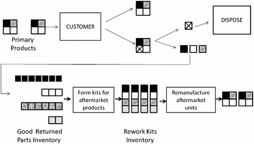
The term ‘re-manufacturing’ has been used to imply many different meanings. Thierry et al. (1995) provide distinctions among various product recovery functions such as re-manufacturing, recycling, refurbishing and cannibalisation. Blackburn et al. (2004) define re-manufacturing and refurbishing interchangeably to mean returning the product to original specifications. Tani (1999) has summarised a comprehensive recycling concept in a graph denoted as the ‘Comet Circle’. In the Comet Circle, recycling at different stages has been labelled as in-house recovery, product recovery, part recovery and material recovery. However, considering many definitions that have been cited in the literature, there seems to be no universal agreement on the recycling terminology. In this paper the term Re-manufacturing is specifically referred to one aspect of recycling as the process of disassembling, separating good and bad parts and using good parts to feed a supply chain for producing discounted after-market products. In this process, each reassembled product assumes a new identity. Figure 1 presents a graphical depiction of this process.

Figure 1 Graphical presentation of the problem.

Even though there are many similar aspects among repair/refurbishing and recycling/re-manufacturing of products, there are a number of differences that justify separate attention to this production situation. To begin with, in these situations the returned parts are new or almost new and can be assembled into products which could function and last as much as a new unit even though it may not be legally possible to sell them as new. Second, the return time is short and often parts are not subject to obsolescence due to model changes. Furthermore, the flow of returned parts is higher and more manageable during the early introduction into the market. This allows reasonable sizes of returned parts inventories to be collected for re-manufacturing production runs. In addition, companies may use this situation to calibrate their targeted production precision by satisfying their demand with a combination of the primary and re-manufactured products.

The deciding factor for even attempting a re-manufacturing scenario is the production cost for each unit of the after-market product. Obviously if the cost to produce after-market products is more than that to produce a primary product, there will not be much incentive to produce or purchase such products. Consequently, one of the main contributions of this paper is to present a methodology to develop a cost function for a re-manufactured product. The second objective is to use this cost function to estimate the breakeven point for primary production rate for which re-manufacturing could be justified.

Some of the factors that contribute to low cost of after-market products are as follows:

•	Availability of returned parts and subassemblies at little or no additional cost.
•	Savings in disposal expenses. These savings tend to be more significant as more environmental protection laws are put in place and enforced.

Factors that may cause the cost of after-market products to go up include:

•	Cost of disassembly of the returned products and sorting of the parts.
•	Increase in reassembly costs due to smaller batch sizes and the need to use alternative manufacturing (assembling) processes compared with those used in manufacturing of primary products.
•	Inventory holding costs for recovered parts until reasonable number of completed kits are accumulated to start a re-manufacturing run.
•	After-market product discount that has to be included in the total cost.

A major factor influencing the re-manufacturing decision is the production rate of the primary product and fraction of defectives of its component parts. Larger production volumes and larger defective rates result in a larger supply of returned parts. This creates a better opportunity for after-market production runs and a higher level of urgency for solving disposal problems. However, the exact level of primary production volume and defective rates that justify after-market production runs is influenced by many other production and environmental constraints.

Many intuitive conclusions could be drawn from the relationship between the breakeven primary production rate and justification of after-market production. For instance, it is clear that stricter disposal regulations would favour after-market production runs for even low primary production rates. Higher rates of defective parts used in production will increase the volume of the returned products and parts, again justifying after-market production for lower production rates. Longer accumulation periods for returned parts will result in larger lot sizes for after-market products for the same primary production volumes, thus making after-market production cost more affordable. However, all these conclusions, although correct, are qualitative in nature and do not provide specific decision rules for a given production environment.

This paper presents a quantitative decision tool for estimation of the unit production cost as a function of all parameters governing the production system. This cost function is then utilised to determine the breakeven point for the primary production rate that justifies attempting re-manufacturing production runs. Changes in the breakeven point are also discussed as production and manufacturing environments change.

Knowing this breakeven point could prove to be very valuable for a manufacturer. It will specifically clarify whether a given production operation could benefit from the re-manufacturing option. Furthermore, additional discussions provided on the sensitivity of this breakeven point to production parameters will provide much useful information to managers to consider producing at production rates that will allow them benefit from re-manufacturing. Although it is true that re-manufacturing will eventually affect the production rate for primary products, this, however, should be considered a desirable outcome for the community as well as for the manufacturer. Because if the manufacturer itself is involved in re-manufacturing of its own products, the total number of units sold and, therefore, the resulting profit remains the same using less raw material and less disposal issues.

The rest of the paper is structured as follows. In Section 2, some definitions used throughout the paper are presented and limitations of the proposed method are discussed. Section 3 presents a brief review of the related work in the literature. In Section 4, the formulation of the problem is provided and relevant functions are derived. Section 5 presents the results of the application of the proposed methodology to a set of alternative scenarios through an illustrative example. Section 6 presents conclusions and suggestions for future research.

2. Definitions and limitations

Materials covered in this paper, clearly, do not apply to all production and product environments. The following definitions will help in understanding circumstances considered in this paper.

2.1 Definitions

Primary products: New products produced in a regular manufacturing operation using new parts utilising most efficient manufacturing and assembly systems available to the company.

After-market products: Products produced solely from reassembling of returned parts or a combination of returned parts with addition of new parts.

Good returned parts: Non-defective parts or subassemblies recovered from disassembly of returned products. The paper will use the generic name of ‘part’ to refer to both a single part and a sub-assembly.

Part accumulation period: The period of time good returned parts are accumulated to form a reasonable batch size for complete kits so that an assembly run could be initiated.

Reassembly cost: The cost of all processes used to re-manufacture a unit of after-market product excluding the cost of parts, inventory, disassembly and disposal.

2.2 Assumptions and limitations

•	A product consisting of one or more defective parts is considered defective.
•	All defective products are returned.
•	All returned products are disassembled and good parts are separated and sorted. Bad parts are disposed of.
•	Good returned parts cannot be used in production of primary products, but new parts could be added to the pool of returned parts to complete assembly kits for after-market products.
•	Reassembly cost is assumed to be a decreasing function of the after-market product batch size and stabilises at a certain value as the lot size exceeds a certain limit. The minimum reassembly cost, however, is generally larger than the assembly cost for the primary product.
•	To develop general conclusions, the production cost of a unit of primary product is assumed to be unity and all other costs are expressed in a dimensionless environment as a fraction of this cost.

3. Background and research motivation

The general issue of reusing parts of returned or scrapped products has been studied in many recent publications. The stages at which subassemblies, parts or materials enter into re-production have a major influence on policies adopted by companies. These stages have clearly been defined in Thierry et al. (1995) and re-instated in Mahadevan et al. (2003). They consist of direct reuse, product recovery management and waste management. In particular, product recovery management has been broken into product to part transition stages of repair, refurbishing, re-manufacturing, cannibalisation and recycling. Although these definitions are stated clearly in the above works, they have not necessarily been used universally in the literature. Consequently re-manufacturing referred to in this paper was defined again in an earlier part of this paper.

A major portion of references to re-manufacturing products in the literature consist of the cases in which end-of-life policies are implemented; Used products are examined and the worn-out components are either replaced by new components or repaired. Although we do not address this issue in this paper, one could refer to Thierry et al. (1995), Ferrer and Jayashankar (2006), Parlikad and McFarlane (2010) and Plant et al. (2010) and many other articles covering various aspects of re-manufacturing at the end of useful life.

Previous research has shown that re-sorting and re-manufacturing is superior to disposal not only because it is an environmentally friendly policy (Guide and Van Wassenhove 2002) but also because it generates revenue (Meyer 1999; Srivastava 2008). Jin et al. (2007) show that re-manufacturing can be an optimal strategy for the company even if the cost of re-manufactured products is as high as that of the primary products.

Richter and Weber (2001) consider the inventory management for a re-manufacturing system in which there is no difference between the new and re-manufactured products for customers but the set-up costs are different. They focus on minimising the total cost, i.e. the total set-up cost and holding cost for re-manufacturing and manufacturing. The principal problem they address is the timing for the start of manufacturing or re-manufacturing production runs. Liang et al. (2009) present a method for pricing of the returned products. While the cost of returned products is assumed to be negligible in this paper, their results could be useful for consideration for extending the application of the proposed method. Galbreth and Blackburn (2006) have proposed a method for optimal pricing for acquisition and sorting of the returned products. But they too restrict their study to refurbishing and repairing returned products and not to recycling as it is intended in this paper.

Ostlin et al. (2008) have identified seven different types of closed-loop relationships for gathering cores for re-manufacturing. These are ownership-based, service contract, direct-order, deposit-based, credit-based, buy-back and voluntary-based relationships. They have then presented several disadvantages and advantages of these relationships and advocated that selection of the right relationship can result in a better understanding of the management of the closed-loop supply chain and re-manufacturing. This information might be useful in extending the application proposed in this paper since the assumption here is that all cores (returned parts) are sent back to the original equipment manufacturers.

Guide et al. (2003) have presented solutions to pricing of re-manufactured products to optimise the total revenue. Mitra (2007) has expanded these solutions to cases in which more than one level of quality exists for re-manufactured products. These concepts will definitely provide an alternative to our assumption of a fixed discount for re-manufactured products. However, both of these studies apply to repaired and re-furbished products rather than to re-manufacturing as defined in our paper.

Depuy et al. (2007) use the case of a re-manufacturing system as an example of a production planning environment in which components are harvested from returned products (carcasses). Their suggested process is well developed and yields the number of units re-manufactured, identifies the periods of low probability of meeting the demand and the number of new components to be purchased to supplement recovered parts. Nikolaidis (2009) proposes a simple mathematical programming model that can help re-manufacturing companies to make optimal decisions concerning the quantities to be re-manufactured. These results are definitely valuable in motivation of seeking a quantitative approach for quantifying decision rules for re-manufacturing decisions.

More comprehensive reviews on the reverse logistics and reverse supply chain have been provided by Debo et al. (2005), Dowlatshahi (2005), and Rubio et al. (2008). Some additional work has been published which could be useful in estimation of disassembly and sorting costs as well as inventory carrying costs needed to perform the proposed approach in this paper. Among them, one could refer to the research conducted by Das et al. (2000) on the overall economics of the disassembly processes, and in particular the cost of disassembly. Another useful work is that of Akçali and Bayindir (2008) on a multi-factor model to determine the disassembly effort index score which represents the impact of inventory holding cost of the recovered parts in a disassembly and recovery environment.

The cited literature and many others that are not referred to due to lack of space certainly emphasise the role of re-manufacturing of returned or used-up products in productivity and sustainability. They also provide a strong motivation to address the main focus of this research. As stated above, intuitive relationships exist between production rate of primary products and factors favouring re-manufacturing of returned products. This paper presents a quantitative process for estimating the minimum primary production rate that justifies re-manufacturing, considers the impact of introduction of new parts to complete re-manufacturing kits and explores the effect of inventory carrying cost on the re-manufacturing decision.

4. Problem formulation

Formulation of the problem consists of two parts. In the first part a relationship is developed for estimation of the costs for a unit of after-market product as a function of the cost of production of a unit of primary product. In the second part, the breakeven point is estimated for a variety of scenarios at which production of after-market product is justified. The problem is formulated in a dimensionless environment. It is assumed that the production cost of a unit of primary product is unity and all other costs are stated in terms of fractions of the unit primary product cost. Components of the cost are then defined for a re-manufactured product and are used to compare the costs for the primary and after-market products for any given primary production rate and production conditions. Breakeven points are then estimated as the primary production rates at which after-market products are economically competitive.

4.1 Estimation of primary and after-market products costs

4.1.1 Primary product cost

The cost for a unit of primary product is expressed as

where

	C PrimaryProduct is the unit primary product cost,
	K is the number of parts in the product,
	C Part_k ; k = 1,K, is the cost of part k as a fraction of unit primary product cost and
	C PrimaryAssembly is the primary product assembly cost as a fraction of unit primary product cost. This cost includes the cost of all processes employed to build a unit of product except the cost of individual parts and subassemblies.

4.1.2 After-market product cost

The cost structure for after-market products is different from the above. Without loss of generality, we assume parts are available at no cost except for the cost of their disassembly and sorting. However, even with free parts the cost of after-market products may still be higher than the cost of primary products due to higher reassembly process cost, cost of disassembling and sorting of parts from returned products, and the inventory holding costs of recycled parts. Furthermore, since these products will be sold at after-market prices, the discount should be considered as another cost item. In cases in which disposal costs are significant, the cost of disposal is subtracted from the cost of after-market products.

Then the cost of a unit of a after-market product, in terms of fractions of the unit primary product cost, can be stated as

where

	C After-market represents unit after-market product cost,
	C Reassembly represents unit reassembly cost,
	C InventoryCarrying represents unit inventory carrying cost per unit time allocated to the set of parts used in each after-market product,
	C Disassembly represents unit disassembly and sorting cost allocated to each after-market product,
	C Discount represents unit discount cost and
	C Disposal represents unit disposal cost.

4.1.2.1 Unit reassembly cost (C _Reassembly)

We assume that good parts recovered from returned products are sorted and placed in kits for each unit of after-market product. We also assume that these kits are accumulated for a fixed period of time, part accumulation period, to form a reasonable lot size for starting an after-market production run as well as to accommodate regular scheduling plans. We also assume that the reassembly cost for each after-market unit is a decreasing function of the batch size of the accumulated kits. Thus the size of these batches needs to be estimated from system's parameters.

The lot size of batches of these kits is clearly a stochastic function of the primary production rate and the percent defective rate of each part type. This lot size is also a function of the accumulation period as well as the way parts match to form a kit. Thus the function to estimate this lot size can be stated as

where

	L After-market represents after-market production lot size,
	R PrimaryProduct represents primary production rate,
	P FailureRate (P Failurerate_k , k = 1,K) represents a vector of failure rates of parts and
	T Accumulation represents accumulation period.

The above relationship does not explicitly address the matching mechanism for parts to form kits; this is a complicated stochastic process. The process to incorporate this factor will be discussed later.

The decreasing function relating the unit reassembly cost to the after-market production lot size, C _Reassembly = r(L _After-market), can take many forms depending on the processes used for re-manufacturing, but, in general, it will eventually be stabilised at a value beyond which the cost does not change. Also it is reasonable to assume that its minimum value, in general, will be greater than the assembly cost for the primary product. We will approximate this cost with a decreasing hyperbolical function. Other functions can also be considered. In an exploration of various functions, we did use a decreasing multistage step function which showed similar results. Once again to preserve the dimensionless nature of the problem, we state the reassembly cost as a product of a multiplier and the assembly cost for the primary product. That is

where M _{Reassembly_l} is the unit reassembly cost multiplier for lot size l = L _After-market and C _Reassembly and C _{PrimaryAssembly} are unit assembly costs for the after-market and the primary products, respectively, as defined above.

Figure 2 illustrates a typical hyperbolically decreasing multiplier function for the after-market products assembly cost as a function of system parameters. Parameters s, t, v and u are defined as

Figure 2 Hyperbolic re-assembly function.

	v: absolute minimum batch size to consider after-market products;
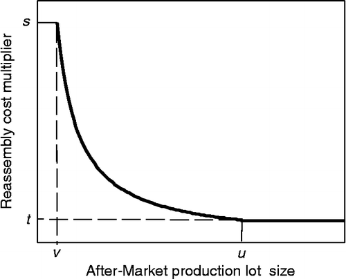	s: multiplier for reassembly cost for a lot size of v;
	u: batch size beyond which unit reassembly costs level off;
	t: multiplier for assembly cost for lot sizes greater than u.

A hyperbolical decreasing cost function multiplier will have the general form as

for values within v and u and of a fixed value for batch sizes larger than u. Parameters a and b can be estimated from the values of s, t, u and v as follows:

The hyperbolical assumption for the cost multiplier will be a good approximation if reassembly cost per unit is assumed to consist of a one-time cost due to the set-up plus a fixed cost per unit.

4.1.2.2 Unit inventory carrying cost (C _{InventoryCarrying})

Inventory carrying costs for good parts allocated to each after-market product can be estimated as follows:

•	Set a planning period.
•	For this planning period, estimate the time each part spends waiting before it is reassembled into an after-market product.
•	Multiply the holding time of each part by its corresponding inventory carrying cost per unit per unit time.
•	Add all these costs and then divide the results by the total number of after-market products produced during the planning period.

4.1.2.3 Unit disassembly and sorting cost (C _Disassemble)

Disassembly and sorting costs apply to all returned products. The number of after-market products is smaller than the number of returned products (due to discarding of bad parts). Thus the contribution of these costs to the unit cost of each after-market product has to be estimated by adding the costs for disassembling and sorting of all returned products and averaging the total over the number of after-market units produced.

4.1.2.4 Unit discount costs (C _Discount)

Discount costs are fixed values which will be estimated based on market demands. These costs are added to the cost of each after-market product.

4.1.2.5 Unit disposal costs (C _Disposal)

If the disposal cost of each returned product (the cost of disposing all of the parts of a unit of product) is C _Disposal, each after-market product causes a savings equal to the disposal cost of a whole unit. In other words the actual cost of each re-manufactured unit is reduced by an amount equal to the cost of disposing one product. As a result this cost should be deducted from the cost of an after-market product.

4.2 Estimating the breakeven point for primary production rate

Since the cost for a unit of primary product is set as unity, the breakeven point for the primary production rate at which recycling is justified, p _break, can be estimated by

where represents the cost of a unit of after-market product for a primary production rate of .

In the following section we describe the computation procedures for estimating the cost elements of a unit of after-market product as a function of primary production rate and system parameters. As stated previously, system's parameters include: the primary production rate, parts' failure rates, discount rate, disposal costs and part accumulation period. Plotting this cost versus various values of primary production rates will result in a guide for estimating the breakeven point for primary production rate at which production of after-market products is justified. This procedure will be demonstrated through an application to a numerical example.

4.3 Computation process

As stated above in order to estimate the cost of an after-market product, several variables representing characteristics of the system have to be estimated. These include the lot size for after-market products, inventory levels for returned parts and allocation of inventory, disassembly, sorting and disposal costs to each after-market product. These characteristics are often results of interactions among some of the following stochastic processes within the system:

•	Many parts may have to wait for a long time until they are matched into a complete kit.
•	There is a complicated inventory process for waiting parts.
•	Arrival and compilation of complete kits for assembly is a random process.
•	A product may have more than one failed part.

Theoretically we can estimate some of these parameters. For instance the rate at which returned products arrive can be estimated from the failure rates of parts. Assuming that each returned product must have at least one failed part, the probability that a product is defective can be estimated as

where β _k is the failure rate for part k. The return rate for a given part, RRU _k , can be stated as

Although the arrival rate of the returned units is helpful in this analysis, it does not quite determine when a good part type is available to complete a kit for reassembly. Furthermore, since the arrivals of good and bad parts are random, queues will be formed of some good parts waiting for other good parts to form complete kits. Estimating parameters of these Queueing systems and the values of all corresponding variables require a closed form solution to a stochastic problem that might be hard to obtain. The alternative is to use a simulation model that estimates all of the above parameters and integrates all prevailing conditions to provide the cost of a unit of after-market product for any given primary production rate.

The structure of the simulation model developed in this study is demonstrated in Figure 3. The following is a description of major steps of this model:

Figure 3 Computation process for unit cost of an after-market product.

•	Steps 1–5 estimate the lot sizes for re-manufacturing after-market products and the unit cost involved for each product.
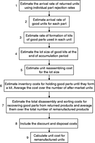•	Step 6 keeps track of individual good returned parts and their time of arrival. At the end of each period, duration of stay for each part is multiplied by its unit inventory carrying cost. The total cost is then divided to the total number of after-market products produced during that period to obtain the share of individual parts of the inventory cost.
•	Step 7 performs a similar operation by adding up all disassembly and sorting costs for all returned products and averaging them over the total number of after-market products produced over the period.
•	At Step 8, the discount is added to the after-market product as an additional cost. Also, since production of each after-market product saves the disposal cost for a unit of product, the actual cost of an after-market product is reduced by this amount.
•	Step 9 adds all the costs to obtain the cost of a unit of after-market product.

4.4 Comparison of costs and the solution approach

Having the estimate of the cost for after-market products in terms of the production rate and cost of primary products makes estimation of the breakeven point a rather easy process. In general, if this function is plotted against the primary product production rate, its intersection with a horizontal line of unity (cost of the primary product) provides the coordinates of the breakeven point.

5. Application of the proposed methodology

In this section the results of application of the proposed method to a numerical example are presented. In particular, first a baseline scenario is presented and the breakeven point is calculated. Then a variety of other scenarios are tested by changing parameters of the system and the results are compared with the base scenario.

5.1 An illustrative example

The primary product being considered consists of an assembly of five parts (subassemblies) each with a 1% chance of being defective. Without loss of generality, we assume that all defective products are returned. Additional parameters of the system stated as fractions of the unit cost of the primary product are as follows:

•	Primary product cost = 1.00.
•	Assembly cost per unit of primary product = 0.20.
•	Total cost of all parts in a unit of primary product = 0.80.
•	Discount for after-market units = 0.20.
•	Inventory carrying cost per unit per period = 0.001.
•	Disassembly and sorting costs for each returned product = 0.1.

5.2 Scenario 1: baseline scenario

For this scenario, we assume that there is no disposal cost and the rest of the parameters are as follows:

	v: Minimum re-manufacturing lot size = 10.
	u: Lot size beyond which reassembly cost does not change = 100.
	s: Reassembly cost multiplier for a lot size of 10 = 6.5.
	t: Reassembly cost multiplier for a lot size of 100 = 2.0.
	β k  = 0.01 and 0.02; k = 1, 5.

Parameters for the hyperbolical cost function multiplier can be estimated using Equation (6) as

Based on the above parameters this cost function is determined as

Using these parameters in the computer simulation model using ARENA produced after-market product costs for various values of the primary production rate and the two values of defective rates. The results are the averages of 20 runs each executed for a year. A year is considered as 50 weeks of 40 h each. Production rates are stated in terms of the number of products per week. Figure 4 shows the corresponding graphs. The half length of a 95% confidence interval for this number of replications averages to about 1% of the mean for most of primary production rates, giving a confidence range of ± 2% of the averages plotted in the graph. A sample of this calculation for the production rates ranging from 500 to 3000 is shown in Table 1.

Figure 4 Breakeven points for hyperbolical distribution for two defective rates.

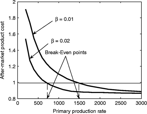
Table 1 Sample percent deviations on the estimates of after-market products cost.

Production rate	800	900	1000	1100	1200	1300	1400	1500	1600	1700	1800	2000
Average cost	1.180	1.139	1.102	1.074	1.047	1.025	1.007	0.990	0.976	0.963	0.952	0.932
σAveragecost	0.069	0.063	0.060	0.056	0.050	0.045	0.042	0.037	0.035	0.032	0.029	0.027
σ/average	0.015	0.014	0.013	0.012	0.011	0.010	0.009	0.008	0.008	0.007	0.006	0.006

As indicated in the figure, the breakeven point for the primary production rate for these alternatives is around 1450 and 700 units per week for defective rates of 0.01 and 0.02, respectively. In other words, if the primary production rate is higher than the breakeven point for each case, after-market products' costs will be less than those of the primary products, justifying the after-market option. Clearly, as expected, higher defective rates for parts justify production of after-market products for lower primary production rates.

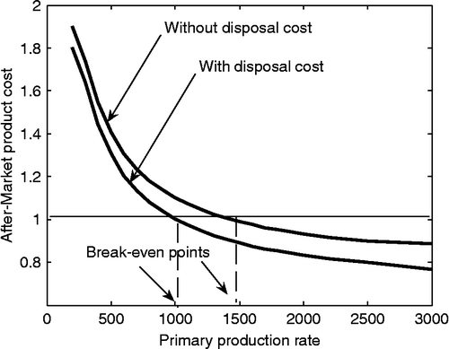
5.3 Scenario 2: impact of disposal cost

In this scenario, a disposal cost of 0.1 was considered for disposing of a whole product. Since re-manufacturing of each unit saves the cost of a whole unit; the cost of each re-manufactured product is reduced by this amount. Figure 5 shows the comparison of the breakeven point for the cases with and without disposal cost. Corresponding values are about 1000 when there is a disposal cost compared to about 1450 when disposal is free. Once again the intuitive answer for this situation was obvious; disposal cost favours re-manufacturing, but the proposed method provides the actual quantitative results for making a decision.

Figure 5 Breakeven point with and without disposal cost.

5.4 Scenario 3: addition of new parts to form complete kits

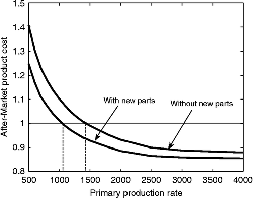
Waiting for accumulation of enough returned parts to form a reasonable batch size may cause a large number of returned parts to be held in an inventory until they are matched with other parts to complete a kit. In fact it can be proved that even with equal fraction defective rates for all parts, the inventory of parts with no match will be unbounded. Our simulation model confirmed this property; longer runs provided larger differences between queue lengths of returned parts. As a result, remaining parts would either have to be disposed of at a disposal cost or be kept for the next cycle, adding to the inventory holding costs. This problem could be resolved if at the end of the accumulation period good return parts are supplemented with sufficient number of new parts so that all returned parts form complete kits and leave the inventory. This action may balance the cost of adding new parts with the savings in inventory cost of returned parts.

Figure 6 presents the comparison of the unit cost of an after-market product for cases with and without added new parts. The results for this comparison indicate that addition of new parts reduces the breakeven point of primary products from about 1450 to about 1100. In fact in this particular example, adding new parts tended to be more cost effective in all cases.

Figure 6 Breakeven points with and without addition of new parts.

To see alternatives for other levels of inventory carrying costs, the model was run for the same primary production rates using inventory carrying costs ranging from 0.0001 to 0.001. Figure 7 shows one of these experiments with an inventory carrying cost of 0.0003. Here for some levels of primary production rate, not adding new parts is more advantageous. This figure also shows the difference between breakeven points for cases with and without addition of new parts.

Figure 7 After-market product cost for an inventory carrying cost of 0.003 as a function of primary production rate.

Table 2 represents a different version of these results for a set of primary production rates and inventory carrying costs. The value in each cell is calculated as

where ΔC _After-market is the difference between the unit after-market product cost without and with addition of new parts. For a given primary production rate and inventory carrying cost, this table provides a guide to decide whether adding new parts is advantageous. All positive numbers indicate that adding new parts results in lower cost for after-market products, while negative numbers show lower unit cost for not adding new parts.

Table 2 Re-manufactured product cost differences for variable inventory carrying costs.

	Inventory carrying cost
Primary production rate	0.0001	0.0002	0.0003	0.0004	0.005	0.0006	0.0007	0.0008	0.0009	0.001
800	− 0.013	0.000	0.013	0.027	0.040	0.053	0.067	0.080	0.093	0.107
900	− 0.015	− 0.003	0.010	0.023	0.035	0.048	0.061	0.073	0.086	0.099
1000	− 0.020	− 0.008	0.004	0.017	0.029	0.041	0.053	0.065	0.077	0.089
1100	− 0.020	− 0.008	0.003	0.015	0.027	0.038	0.050	0.061	0.073	0.084
1200	− 0.022	− 0.012	− 0.001	0.010	0.021	0.032	0.043	0.054	0.065	0.076
1300	− 0.023	− 0.013	− 0.002	0.008	0.018	0.029	0.039	0.049	0.060	0.070
1400	− 0.024	− 0.014	− 0.004	0.006	0.016	0.026	0.036	0.046	0.056	0.066
1500	− 0.025	− 0.015	− 0.006	0.004	0.014	0.023	0.033	0.042	0.052	0.061
1800	− 0.025	− 0.017	− 0.008	0.000	0.009	0.017	0.026	0.034	0.043	0.051
2000	− 0.026	− 0.018	− 0.010	− 0.002	0.006	0.015	0.023	0.031	0.039	0.047
2500	− 0.027	− 0.020	− 0.013	− 0.006	0.001	0.008	0.015	0.022	0.029	0.036
3000	− 0.028	− 0.022	− 0.015	− 0.009	0.003	0.003	0.010	0.016	0.022	0.029

5.5 Scenario 4: variation of part accumulation period

Increasing the length of accumulation period before starting an after-market production run will allow forming of larger lot sizes, leading to lower unit reassembly costs. However, longer accumulation periods will add to the inventory volume and inventory carrying costs. For each value of the primary production rate, several accumulation periods were experimented with. These experiments were conducted for cases in which no new part was added and after-market products were assembled exclusively from good returned parts. The results of these experiments are presented in Figure 8. Each plot represents a volume of primary production rate as indicated in the legend. Table 3 shows the accumulation periods that result in minimum costs for after-market products for given primary production rates. As the table indicates, the optimum accumulation period increases (shifts to right) as the primary production rate decreases. This makes sense as smaller primary rates will require longer periods for returned parts to form reasonable lot sizes for re-manufacturing runs.

Figure 8 Optimum accumulation period for various production rates.

Table 3 Optimum accumulation periods resulting in minimum re-manufactured product costs.

Primary production rate	2000	2500	3000	3500	4000	4500	5000
Unit re-manufactured cost	0.932	0.9	0.878	0.865	0.849	0.839	0.835
Accumulation period: hours (days)	40 (5)	40 (5)	32 (4)	32 (4)	24 (3)	24 (3)	24 (3)

6. Conclusions and suggestions for future research

This study presented a quantitative approach for making decisions on recycling of the good parts recovered from returned products to after-market products that could be sold at discount. It addressed the complicated issue of estimating the flow of parts in the reverse supply chain of recovered good parts from returned products to form reasonable batch sizes for an after-market production run. A methodology was presented to estimate the cost of the after-market products for various production and manufacturing environments for the system as a function of the primary production rate. Operation parameters considered included the defective rates of original parts, cost of disposal of returned products, the impact of mixing returned parts with new parts to complete kits for after-market products and the impact of varying the accumulation period for returned parts. The cost of after-market product as a function of the primary production rate was then used to determine the volume of the production at which introduction of after-market products could be justified.

The proposed method was developed using a number of relatively reasonable assumptions for the production and cost parameters. However, several of these assumptions could be reconsidered for additional research in this field. For instance the nature of accumulation of parts that never find enough matches to be utilised is an interesting subject that is being considered by the authors. Although it is expected that the inventory levels will rise when defective rates of original parts are different, our preliminary research has indicated that even with the same values of defective rates for all parts, still the difference in the volume of good returned parts will not be bounded. Additional promising area is the development of close form solutions for some of the critical aspects of the problem. There are possibilities that product and production processes could be designed such that satisfying the demand with the combination of primary and after-market products would result in a lower total cost. These issues are being addressed by the authors and will be published when completed.

Additional information

Notes on contributors

Sharon Ordoobadi

1

Notes

1. Email: [email protected]

References

- Akçali , E. and Bayindir , P.Z. 2008 . Analyzing the effects of inventory cost setting rules in a disassembly and recovery environment . International Journal of Production Research , 46 ( 1 ) : 267 – 288 .
- Blackburn , J.D. , Guide , V.D.R. , Souza , G.C. and Van Wassenhove , L.N. 2004 . Reverse supply chain for commercial returns . California Management Review , 46 ( 2 ) : 6 – 22 .
- Das , S. , Yedlarajiah , P. and Narendra , R. 2000 . An approach for estimating the end-of-life product disassembly effort and cost . International Journal of Production Research , 38 ( 3 ) : 657 – 673 .
- Debo , L.G. , Toktay , L.B. and Van Wassenhove , L.N. 2005 . Market segmentation and product technology selection for remanufacturable products . Management Science , 46 ( 8 ) : 1193 – 1205 .
- Depuy , G.W. , Usher , J.S. , Walker , R.L. and Taylor , G.D. 2007 . Production planning for remanufactured products . Production Planning & Control , 18 ( 7 ) : 573 – 583 .
- Dowlatshahi , S. 2005 . A strategic framework for the design and implementation of remanufacturing operations in reverse logistics . International Journal of Production Research , 43 ( 16 ) : 3455 – 3480 .
- Ferrer , G. and Jayashankar , J.M. 2006 . Managing new and remanufacturing products . Management Science , 52 ( 1 ) : 15 – 26 .
- Galbreth , M.R. and Blackburn , J.D. 2006 . Optimal acquisition and sorting policies for remanufacturing . Production and Operations Management , 15 ( 3 ) : 384 – 392 .
- Guide , D.V.R. and Van Wassenhove , L.N. 2002 . The reverse supply chain . Harvard Business Review , February : 24
- Guide , V.D.R. Jr. , Teunter , R.H. and Van Wassenhove , L.N. 2003 . Matching demand and supply to maximize profits from remanufacturing . Manufacturing & Service Operations Management , 5 ( 4 ) : 303 – 316 .
- Jin , Y. , Muriel , A. and Lu , Y. 2007 . “ On the profitability of remanufactured products ” . In Presented at the 18th annual conference of POMS , May 4–7, Dallas, TX, USA
- Liang , Y. , Pokhare , S.l. and Geok Hian Lim , G.H. 2009 . Pricing used products for remanufacturing . European Journal of Operational Research , 193 : 390 – 395 .
- Mahadevan , B. , Pyke , D.F. and Fleischmann , M. 2003 . Periodic review, push inventory policies for remanufacturing . European Journal of Operational Research , 151 : 536 – 551 .
- Meyer , H. 1999 . Many happy returns . Journal of Business Strategy , 80 ( 7 ) : 27 – 31 .
- Mitra , S. 2007 . Revenue management for remanufactured products . Omega , 35 : 553 – 562 .
- Nikolaidis , Y. 2009 . A modelling framework for the acquisition and remanufacturing of used products . International Journal of Sustainable Engineering , 2 ( 3 ) : 154 – 170 .
- Ostlin , J. , Sundin , E. and Bjorkman , M. 2008 . Importance of closed-loop supply chain relationships for product remanufacturing . International Journal of Production Economics , 115 : 336 – 348 .
- Parlikad , A.K. and McFarlane , D. 2010 . Value of information in product recovery decisions: a Bayesian approach . International Journal of Sustainable Engineering , 3 ( 2 ) : 106 – 120 .
- Plant , A. 2010 . Design standards for product end-of-life processing . International Journal of Sustainable Engineering , 3 ( 3 ) : 159 – 169 .
- Richter , K. and Weber , J. 2001 . The reverse Wagner/Whitin model with variable manufacturing and remanufacturing cost . International Journal of Production Economics , 71 : 447 – 456 .
- Rubio , S. , Chamorro , A. and Miranda , F.J. 2008 . Characteristics of the research on reverse logistics (1995–2005) . International Journal of Production Research , 46 ( 4 ) : 1099 – 1120 .
- Srivastava , S.K. 2008 . Network design for reverse logistics . International Journal of Management Science , 36 : 535 – 548 .
- Tani , T. 1999 . “ Product development and recycle system for closed substance cycle society ” . In Proceedings of First International Symposium on Environmentally Conscious Design and Inverse Manufacturing 294 – 299 . February 1999, Tokyo, Japan
- Thierry , M. 1995 . Strategic issues in product recovery management . California Management Review , 37 ( 2 ) : 114 – 135 .