Abstract
For many manufacturers, the cost of replacing returned products may more than offset the cost of producing parts with a higher quality. This is especially true if good parts from returned products are used to remanufacture aftermarket products. Furthermore, such policy allows for satisfying a customer population with a variable expectation for acceptable quality. In this study, the total cost of supplying a given demand is derived as an analytical function of the targeted primary production rate and product quality when the demand is satisfied with a combination of primary and remanufactured products. The decision variables of this function consist of the primary production rate and the designed product and production quality. This cost is then minimised to determine the production rate and the optimum quality to target. A numerical example is provided and used to demonstrate the application of this function. This example also demonstrates the use of the proposed solution for optimising quality when there is a limit on primary production size. The example also demonstrates the use of the function for optimising service levels. The results show a close match between the theoretical functions developed in this study and those obtained from a Monte Carlo simulation model.
Introduction
To be competitive in the market, many companies have adopted a ‘no question asked’ return policy. Although this policy has its cost drawbacks, this study proposes a strategy that could take advantage of this to optimise a flexible quality target. Clearly, manufacturing products that are 100% free of defective parts necessitate very high-quality standards for the design and manufacturing processes with exceedingly high production costs. Aiming at such quality does not necessarily achieve the desirable goals of quality and affordability. Customers have different levels of expectations and a quality level that pleases one customer may turn out to be overkill to another customer. Easy return policies coupled with remanufacturing of good returned parts may satisfy the flexible customer quality expectations, while minimising the total cost. Furthermore, reusing return parts will address sustainability and environmental considerations.
This study suggests a procedure in which the customers' level of expectation plays a role in designing of the quality of parts used in the product. The general idea here is that rather than committing to high costs of minimising the product failure, the manufacturer allows an easy replacement of a product, which fails within a specified period, with a new product. Good parts recovered from returned products are then used to manufacture aftermarket products. As the definition of ‘failure’ could vary from customer to customer, the result of such a policy would be to satisfy a variable customer choice through a process that eventually may be most cost-effective. In other words, the cost of replacing a product returned by a customer who is not happy with the quality and remanufacturing the returned units may be more than offset by savings resulted from manufacturing batches that are less perfect but still satisfy a good portion of customer population.
Naturally, this policy is not recommended for every product. The proposed approach is designed for production environments in which:
| • | the production cost (or the production cost of components used in the product) is inversely proportional to the quality (fraction defective rate) of parts used in the product; | ||||
| • | returned products could be disassembled and sorted for good and defective parts and good parts could be recycled into production of aftermarket products; | ||||
| • | the total demand is satisfied by a combination of the primary and aftermarket products; | ||||
| • | the discount provided for an aftermarket product is such that it makes it indifferent for a customer to buy either. Also it is assumed that the customer will be indifferent if the replacement unit is a primary or an aftermarket product since he/she will be refunded with an amount equal to the discount if the returned product was a primary unit and | ||||
| • | parts used in aftermarket products are 100% inspected making them almost defect free, even though this is not well accepted in the market and a discount is still needed. | ||||
The main objective of this study is to search for the level of quality to design in parts and products for minimising the overall cost of satisfying all demands while environmental and sustainability constraints are satisfactorily met. As it will be shown for a given level of demand, the designated quality (percent defective parts used in the product) and targeted primary production rate (products made of original new parts) will determine the probability distribution of the number of returned parts, probability distribution of the number of aftermarket products and the overall cost of satisfying demands. The total cost of production includes the cost for the primary and aftermarket products as well as a shortage penalty for the portion of the demand that is not satisfied.
It is expected that this research will open several new avenues for looking at the targeted design quality from different perspectives. It addresses the possibility that some sacrifices in the level of production quality may indeed result in a lower total production cost to meet demands satisfactorily. An additional aspect of this approach is the advantage a manufacturer can gain by utilising customers as components of its flexible quality inspection workforce (as customers use different criteria for acceptability of the same product) and supply different customers with quality tailored for their preferences. Furthermore, recycling of returned products will serve the sustainability requirements. A numerical example is provided and used to demonstrate the application of developed functions. This example also demonstrates the use of the proposed solution for optimum quality when there is a limit on primary production size. The example also shows how the proposed solutions could be used to design for optimum service levels. Solutions resulted from this example are compared with those obtained from a simulation model. The results show a very close match between analytical and simulation results.
Literature review
The trade-offs between the production costs and customer satisfaction through return and warranty policies have been studied extensively in the literature. However, the assumption has usually been that the rejected products are discarded and can easily be disposed of. With increased sensitivity to sustainability and environmental concerns, the economic and political landscapes have changed drastically and continue to change at an even faster rate.
The dominant references to remanufacturing products in the literature consist of the cases in which end-of-life policies are implemented, used products are examined and the worn-out components are either replaced by new components or repaired. Although this issue is not addressed in this study, for a sample, one could refer to Thierry et al. (Citation1995) and Ferrer and Swaminathan (Citation2006) and many other articles covering various aspects of remanufacturing at the end of useful life.
Previous research has shown that resorting to remanufacturing is superior to disposal not only because it is an environmentally friendly policy (Guide and Van Wassenhove Citation2002) but also because it generates revenue (Meyer Citation1999, Srivastava Citation2008). Jin et al. (Citation2007) show that considering remanufacturing can be an optimal strategy for the company even if the cost of remanufactured products is as high as those of the primary products.
Adding remanufacturing concept into the supply chain affects both supply and demand. Much research has been done to estimate and quantify this effect by estimating the number of remanufactured products. Jayaraman et al. (Citation1999) developed a 0-1 mixed integer programming model to identify the optimal reverse production and stock quantities for a company that utilises both reverse and forward flows to satisfy the demand. They used repaired components of used products supplemented by new components to form a remanufactured product. The conclusion they come up with is that the number of cores available for remanufacturing products is a key variable that should be considered for starting a remanufacturing line. Depuy et al. (Citation2007) developed a model to estimate the expected number of remanufactured products at each manufacturing period. To do so, they used a probabilistic standard material requirement planning. They also studied the delays if the good components of returned products needed to be supplemented by new components.
Primary product demand cannibalisation is one of the other effects of remanufacturing on the supply chain. Debo et al. (Citation2005) and Ferguson and Toktay (Citation2006) discussed the demand cannibalisation resulting from selling the manufactured and remanufactured products in the same market. Debo et al. (Citation2005, Citation2006a,Citationb) studied this cannibalisation for a monopolist manufacturer with an attempt to set the price of both new and remanufactured products to maximise the profit. Mitra (Citation2007) considers the case in which remanufactured products are of different qualities and thus have different pools and consequently different prices. He then tries to maximise the expected revenue of the firm under this assumption.
Another important decision variable for planning the production of remanufactured products is the manufacturing period the remanufactured products will be aimed for. Because of the time it takes for the cores to be gathered for remanufacturing, often two-period or multi-period models are developed in which the remanufacturing is only planned for the second period onwards. Ferrer and Swaminathan (Citation2006) proposed a model to study a firm that manufactures only new products in the first manufacturing period and then utilises the returned cores to form the remanufactured products for the following manufacturing period in a monopoly environment. Majumder and Groenevelt (Citation2001) give the manufacturer the option to make a decision whether to do the remanufacturing in the second period or not.
There are several differences in the focus of this research compared to what was mentioned above. Remanufactured products here are defined specifically as reassembling good parts of products returned just a short time after they are delivered to customers. Azadivar and Ordoobadi (Citation2012) have addressed a similar situation but the focus of their work was on estimating the production volumes that justify remanufacturing. Similarly, most of the studies mentioned above treat different aspects of remanufacturing and mix of new and remanufactured products to satisfy the demand or maximise profit in a market with a fixed quality expectations. The most distinctive difference between this study and other studies in the literature is utilisation of remanufacturing function as a means of designing the product and its production such that the profit is maximised in a market with variable quality expectations. This approach will determine the production quality and production volume that will satisfy the demand for all customers such that savings resulted from satisfying least demanding customers will more than upset the cost of providing a perfect product for more choosy customers.
Problem definition
The problem being addressed in this study is defined in the following environments.
There is a specific volume of demand for each period that is satisfied by a combination of primary and aftermarket products manufactured in that period. Each period starts with a batch of new parts for production of primary products and an inventory of good returned parts from the previous period ready to be remanufactured into aftermarket products. The decision vector for optimisation consists of the quality of parts in terms of the targeted probability of a given part being defective (which is the same as the percent defective rate for a batch) and the target volume for primary products. A steady-state situation is assumed in which the demand and the distribution of the type of returned products stay the same from period to period.
Demand for a product for each period is designated by D. N P primary products are manufactured in each period using new parts. Each product is the result of assembling n different part types. The production cost of component i is a function of its quality in terms of the probability, p i , that a given part in the batch is defective. Table displays the list of variables used in this study.
Table 1 List of variables.
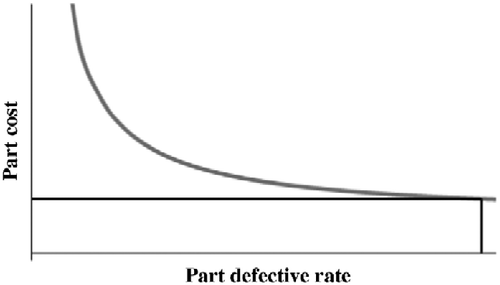
Although it is clear that the cost per part is a decreasing or at least non-increasing function of the parts' quality, the actual form of this function varies depending on production and design conditions. As the first approximation, in this study, parts' costs are assumed to be hyperbolic functions of their defective rates. For a practical range of p, this cost can be derived from the function depicted in Figure .
Figure 1 Part cost as a function of part defective rate.
N R is the number of primary manufactured products that are returned by the customers during T. It is assumed that returned products are disassembled and good parts are sorted and stored in the inventory until the start of the next production cycle. The number of aftermarket or remanufactured products assembled in each period is denoted by N A. At the end of the period, good parts that do not find matches to be reassembled into a remanufactured product can be supplemented by new parts to form the appropriate kits, are kept for the next period or are disposed. In this study introduction of new parts has not been considered.
As stated earlier, the demand for the period is assumed to be satisfied by a combination of the primary and aftermarket products. The final number of products that can contribute to satisfaction of the demand (or N T) is given by
In this equation N p, a decision variable, is a deterministic variable whereas N T, N R and N A are random variables resulting from the stochastic nature of the system.
To find the (p i , N P) vector that maximises the total profit of the system, the distribution of the following variables and their expected values are required:
| • | N R | ||||
| • | N A | ||||
| • | (N R–N A) | ||||
| • | N T. | ||||
Without loss of generality from now on, we assume that the product consists of one of each part type. Furthermore, it is assumed that the designed fraction defective rate p i = p is the same for all parts. Although without the latter assumption the number of revived good returned parts will be unbalanced and a larger number of extra parts will have to be disposed of, the solution for the problem will remain the same.
Problem formulation
In what follows, the relationship for estimating the total cost and the processes for estimating the parameters needed to estimate this cost is described.
Production cost function
All the costs in the cost function are considered as fractions of the total cost for a unit of the highest possible quality primary product. This quality is defined as the scenario in which the product is assembled from parts with least possible defective rate p min. Cost parameters for primary products are as follows:
| • | C part: cost of all parts per unit of primary product. | ||||
| • | C assembly: assembly cost per unit of primary product. | ||||
| • | C disposal: disposal cost per part. | ||||
Cost parameters for remanufactured products are
| • | C disassembly&sort: cost of dissembling and sorting each returned product. | ||||
| • | C reassembly: cost of reassembling a unit of aftermarket product. | ||||
| • | C inventory: inventory cost for each revived part over period T. | ||||
The total cost function that should be minimised is given by
Notice that the manufacturing of the primary products is considered to be just-in-time and hence no inventory costs have been considered for the primary manufactured products.
The cost of the primary product for the least possible part defective rate p min is assumed to be 1, with C part percentage of it being the part cost and C assembly percentage of it being the assembly cost. The n(N R–N A)C disposal component of C primary is approximated to be zero for p min as it is considered that this cost is unavoidable and exists in all situations. All the other cost components are stated as a ratio of the C primary with the ultimate defective rate, which is approximated to be 1.
Profit function
Since the ultimate goal is to maximise the profit of the manufacturer, the profit functions are defined in Equations (Equation5-7).
α and β in the above formula are the selling prices of the primary and the aftermarket products, respectively.
The objective of this study is to find the combination of (p, N P) such that the total profit P total is maximised.
Computing the required parameters
From the P total function, it is clear that many parameters need to be estimated from the stochastic variables that characterise the system. Following are the derivations.
Distribution of N R
N R has a binomial distribution with parameters N P and 1 − (1 − p) n . Therefore, E(N R ) can be computed as
Distribution of N A
Defining P i,m as the probability that part type i from the mth returned product is defective given that there is at least one defective part in a returned product and K i,m as the number of defective parts of type i gathered from the previous m returned products so far, we will have
P(K i,m − 1 = j) follows a binomial distribution with parameters (m − 1) and p i , so
Assuming each product has one part of type i, manufacturing N P primary products requires N P parts of type i. Since the defective rate of part type i is p i , p i N P is the expected number of defective parts of type i. It means that at the end of production period, the expected number of defective parts of type i will be p i N P. At the stage in which from the N P number of total manufactured products, m − 1 products have been returned, N P-(m − 1) products have not been returned yet. Also, from the expected number of p i N P number of type i parts that will be found defective, j of them have already been found defective, so from the products that will be returned later, p i N P–j are expected to have a defective part of type i. Consequently, we will have
Substituting Equations (Equation10) and (Equation11
) in Equation (Equation9
), we have
Since m is fixed, the numerator can be expanded into two terms,
In order to have N A number of aftermarket products, one of the n different part types should have N A good returned parts and the other (n − 1) part types should have at least N A good returned parts. So P(N A = n a) has two components.
From Equation (Equation13), we know that P
i,m
, which is the probability that part type i from the mth returned product is defective, is equal to
Considering X a variable with a binomial distribution with parameters n r and
So,
Consequently, E(N A) can be computed as follows:
Distribution of (N R –N A )
This distribution can be easily computed using the same approach used to compute Pr(N
A = n
a). The result is displayed in Equation (Equation18).
And E(N
R–N
A) can be computed from Equation (Equation19) below.
Distribution of N T
Using the distribution of N
A from Equation (Equation16), the final equation for the distribution of N
T is displayed as
Numerical examples
In order to demonstrate the application of the proposed method, it is used to solve a numerical example. The details of his example is as follows:
The part cost is assumed to be a hyperbolic function of the part defective rate. p min = 0.01 and p max = 0.99 (the min and max defective rates within the production quality range, respectively) and C min = 0.10 and C max = 0.18 (the min and max part cost associated with p max and p min, respectively) are the values that have been used to compute the parameters of the hyperbolic function.
Table shows the values considered for the other parameters used in this example.
Table 2 Variable values used for the numerical example.
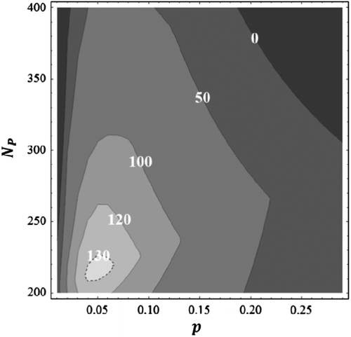
Figure displays the total profit function, P total using Equations (Equation5-7) for p values between 0.01 and 0.3 and the N P values ranging from 200 to 400. Figure illustrates the contour display of P total.
Figure 2 Total profit function.
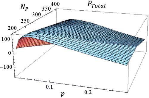
Figure 3 Contour display of the P total function.
Maximisation of profit
As indicated in Figures and , part defective rate of 0.05 and N p of 215 units result in maximum profit. This result is obviously very useful when both defective rates and primary production rates are controllable variables as it provides a definite maximum profit. More careful review of these figures provides additional information on performance of the system, especially when one of these variables is fixed as a given constraint.
Figure (a) shows (the optimum value of N
P) for p values ranging from 0.01 to 0.99. This figure could be utilised as a decision rule for situations in which the percent defective of lots is fixed and uncontrollable. In such situations, for any given percent defective the optimum primary production rate could be obtained from this figure. Up to the defective rate of 0.31,
is an increasing function of p. This is understandable because up to this point the profit for each sold product more than offsets the additional cost of producing more primary products. After the defective rate of 0.31, however, the total cost outweighs the total revenue and thus the production in general is not profitable anymore. This conclusion can be confirmed by observing Figure (b), in which the optimum profit for each defective rate, or
, is plotted against p for the optimum values of
. Here after the defective rate of 0.31, even the optimum value for primary production rate,
, results in a negative profit.
Figure 4 (a) The optimum primary production volume for different part defective rates. (b) The maximum profit for different part defective rates. (c) The optimum part defective rate for different primary production rates. (d) The maximum profit for different primary production rates.
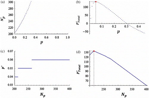
Figure (c) displays p* (the optimum value of p) for N P values ranging from 200 to 400. Again this figure could be used as a decision-making aid in deciding the target quality if the primary production rate is restricted to be a fixed value (perhaps due to restrictions on logical batch sizes!). The optimum value of p for each N P is the value that maximises the total profit for that N P. As Figure (c) indicates, in general, the optimal p value is an increasing function of N P and remains constant for a considerable range of N P. Figure (d) depicts the optimum profit value for each N P, as computed by replacing the N P and the p* values corresponding to that N P in Equations (Equation5-(7). Once again the conclusion is that beyond a certain value for the primary production rate, even choosing an optimum value for p will result in a loss.
Maximisation of service level
Solving the profit maximisation problem helps the manufacturer find the optimal (p, N
P) set at which the total profit is maximised. However, sometimes the goal is not only, or at all, to maximise the profit, but also to satisfy a certain service level. Service level is defined as the percentage of demand that is satisfied. N
T is the total number of primary and aftermarket products available to serve customers for the optimal (p, N
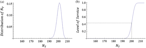
P) of (0.05, 215). The Distribution of NT is displayed in Figure (a). The area under the N
T
distribution curve could be used to demonstrate service levels for various values of primary production rates. This is displayed in Figure (b) for the (p, N
P) set (0.05, 215). As Figure (b) shows, the level of service for N
T of 200, which is the demand in this example, is only around 60%. Thus, although the p*, set of (0.05, 215) maximises the profit, it does not support a high-level of service.
Figure 5 (a) N
T distribution for (p*, ) of (0.15, 215). (b) Level of service for (p*,
) of (0.05, 215).
In circumstances such as above in which the profit and service levels present themselves as two mutually exclusive objectives, the distribution for N T and the resulting service level could be used in a multi-objective optimisation process for maximisation of both profit and service level.
Figure (a) and (b) displays the N T distribution and level of service for the (p, N P) of (0.05, 220), respectively. As it can be observed in Figure (b), for a higher primary production volume of 220 and part defective rate of 0.05, the level of service is increased to more than 96%.
Figure 6 (a) N
T distribution for (p, ) of (0.15, 220). (b) Level of service for (p,
) of (0.15, 220).
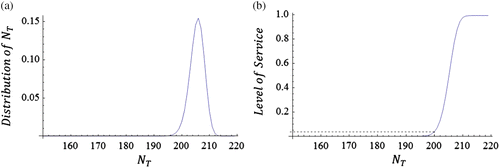
Figure (c) shows that the optimum part defective rate for the primary production volume of 220 is 0.05. The (p, N
P) set of (0.05, 220), as Figure displays, is in the 130 profit contour, and, therefore, to a great extent satisfies the profit objective. So, for the N
P value of 220, not only the profit requirements are satisfied, but also with a very high probability almost all of the demand has been satisfied too. In fact, the expected value of unit shortage for this example, which can be computed using Equation (Equation22), is only 0.03 units.
Comparison with results from a simulation model
A Monte Carlo simulation model was built for the same system for estimating values of P total under similar condition as above. The model was run for part defective range of 0.01–0.3 and for the primary products ranging from 200 to 400. Like before, a product is considered to be a returned product if and only if at least one part of the product is defective. The cost and profit functions used in the simulation program are the same as the cost and profit functions displayed in Equations (Equation2-7), and the other parameters have the same value as given in Table .
Table 3 Variable names and descriptions in the simulation program.
Figure displays the flowchart of the simulation model and Table lists the variables used in the simulation program.
Figure 7 The simulation flowchart.
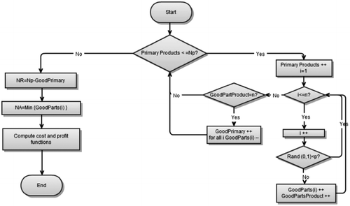
The program generates one primary product at a time until N P is reached. PrimaryProducts is the variable that keeps track of the number of primary products. For each primary product, first it is determined whether each of the n part types is defective. If the part type i is not defective, then the GoodParts(i) and GoodPartsProduct variables are incremented by 1. GoodParts(i) is used to keep track of the number of non-defective parts of type i in all the N R returned products. GoodPartsProduct counts the number of good parts in one primary product only. After all the parts for the primary product were generated, then the value of the GoodPartsProduct variable is examined. If it is equal to n, it means that all parts of the newly added primary product are good. As a result, the GoodPrimary variable, which counts the number of the primary products that are non-defective, is incremented by 1, and each of GoodParts(i)s is decremented by 1.
N R is then computed by subtracting the value of the GoodPrimary variable from N P, and N A is the minimum of the n GoodParts(i) variables.
With values of N P, N R and N A known, Equations (Equation5-(7) can be used to compute the total profit function.
The simulation model was calibrated with the same parameters presented in Table . Ten replications of the model were run and the average results were used to create the contour display of function P total. Figure displays the contour display of the simulation results against that of the analytical model previously presented in Figure .
Figure 8 Comparison of the results of the analytical model with the simulation results.
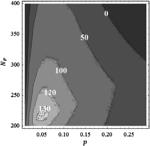
Comparison of the P total function obtained from the analytical and simulation models indicates the similarity between the outputs of the two methods. This similarity is further displayed quantitatively in Table . Error for each (p, NP) set is computed by subtracting the simulation results from the analytical results, and the relative error is computed by dividing the absolute value of the error by the corresponding analytical result. The maximum relative error of less than 4% suggests the congruency of the results by the simulation and the analytical models.
Table 4 Comparison of simulation and analytical models.
Conclusion
This study investigated a production environment in which manufacturers have a policy of providing a replacement for a returned product and recycling good parts recovered from these products in a remanufacturing of aftermarket products. The objective is to maximise profits by targeting a quality goal that maximises the profit while satisfying a variable quality expectation from customers. A model was developed which uses the target quality and the primary production rate as decision variables in a stochastic profit function. This model was then optimised to provide the desired quality to target and the number of primary products to manufacture to maximise the profit. Furthermore, the model was expanded to provide additional results in terms of the service level (percent of satisfied demand) for a given solution.
The results provided indicate many advantages for using this system of production and recycle. Most importantly it indicates that even in environmentally conscious manufacturing circumstances, the design for the highest possible quality does not necessarily result in the best operation policy. Lower design quality targets could be used to maximise profit without sacrificing environmental concerns. Second, this study presents an opportunity to utilise customers as an intelligent and flexible quality control mechanism. Clearly, not all customers have the exact same quality expectations. Since some customers may still be happy with a product with a minor defect, the manufacturer could save the cost of providing perfect products to everybody while still keeping their customers happy.
In addition to the above results, a major contribution of this study is that it provides a rather closed-form solution for a difficult stochastic problem. Simulation analyses have been used before on similar problems and in fact they have also been used in this paper for comparisons. However, a closed-form solution is helpful in confirming the results.
There are many issues that will need further investigations. For instance, the model will need to be expanded to include cases in which new parts could be added to complete the kits for aftermarket products when there is not enough supply of particular good returned part type to complete remaining kits. Another option to search for is the ideal production period that will balance the start-up costs with inventory carrying costs for returned parts.
Additional information
Notes on contributors
Neda Masoud
1Notes
References
- Azadivar , F. and Ordoobadi , S. 2012 . Decision rules for recycling returned products . International Journal of Sustainable Engineering , (to appear, Available online at http://www.tandfonline.com/doi/abs/10.1080/19397038.2011.618561)
- Debo , L.G. , Toktay , L.B. and Van Wassenhove , L.N. 2005 . Market segmentation and product technology selection for remanufacturable products . Management Science , 51 ( 8 ) : 1193 – 1205 .
- Debo , L.G. , Toktay , L.B. and Van Wassenhove , L.N. 2006a . Life cycle dynamics for portfolios with remanufactured products . Production and Operations Management , 15 ( 4 ) : 509 – 513 .
- Debo , L.G. , Toktay , L.B. and Van Wassenhove , L.N. 2006b . Joint life cycle dynamics of new and remanufactured products . Management Science , 15 ( 4 ) : 498 – 513 .
- Depuy , G.W. , Usher , J.S. , Walker , R.L. and Taylor , G.D. 2007 . Production planning for remanufactured products . Production Planning and Control , 18 ( 7 ) : 573 – 583 .
- Ferguson , M.E. and Toktay , L.B. 2006 . The effect of competition on recovery strategies . Production and Operations Management , 115 ( 3 ) : 351 – 368 .
- Ferrer , G. and Swaminathan , J.M. 2006 . Managing new and remanufacturing products . Management Science , 52 ( 1 ) : 15 – 26 .
- Guide , V.D.R. Jr and Van Wassenhove , L.N. 2002 . The reverse supply chain . Harvard Business Review , 80 ( 2 ) : 25 – 26 .
- Jayaraman , V. , Guide , V.D.R. Jr and Srivastava , R. 1999 . A closed-loop logistics model for remanufacturing . Journal of the Operational Research Society , 50 : 497 – 508 .
- Jin, Y., Muriel, A., and Lu, Y., 2007. On the profitability of remanufactured products. presented at the 18th annual conference of POMS, May 4–7, Dallas, TX, USA
- Majumder , P. and Groenevelt , H. 2001 . Competition in remanufacturing . Production and Operations Management , 10 ( 2 ) : 125 – 141 .
- Meyer , H. 1999 . Many happy returns . Journal of Business Strategy , 80 ( 7 ) : 27 – 31 .
- Mitra , S. 2007 . Revenue management for remanufactured products . The International Journal of Management Science , 35 : 553 – 562 .
- Srivastava , S.K. 2008 . Network design for reverse logistics . The International Journal of Management Science , 36 : 535 – 548 .
- Thierry , M. , Salomon , M. , van Nunen , J. and Van Wassenhove , L.N. 1995 . Strategic issues in product recovery management . California Management Review , 37 ( 2 ) : 114 – 135 .