Performance evaluation of the remanufacturing system prone to random failure and repair

ABSTRACT

Implementation of new environmental legislation and public awareness has increased the responsibility of manufacturers. Remanufacturing has been applied in many industries and sectors since its introduction. However, only 10% to 20% of the returned products pass through the remanufacturing process, and the remaining products are disposed in the landfills. Uncertainties like high failure rates of the servers, buffer capacities, and inappropriate preventive maintenance policies would be responsible for most of the delays in remanufacturing operations. In this paper, a simulation-based experimental methodology is used to determine the optimal preventive maintenance frequency and buffer allocation in a remanufacturing line. Moreover, an estimated relationship between preventive maintenance frequency and Mean Time Between Failure (MTBF), is presented to determine the best preventive maintenance frequency. The solution approach is applied to computer remanufacturing industry. Analysis of variance (ANOVA), and regression analysis are performed to denote the most influential factors to remanufacturing cycle time (performance measures). A case study is used to show the applicability of the modelling approach in assessing and improving the cycle time, and the profit of a remanufacturing line . Managerial insights are highlighted to support managers and decision-makers in their quest for more efficient and smooth operation of the remanufacturing system.

KEYWORDS:

• Remanufacturing
• cycle time
• material recovery
• preventive maintenance
• buffer contribution, Experimental design, ANOVA, Recycling,Simulation

1. Introduction

The implementation of rigid environmental legislation and increased public awareness has forced the manufacturers to begin the recycling and remanufacturing of their used products. Remanufacturing is an industrial process that starts with the collection of used products (cores) and restores them to new conditions, and this process allows manufacturers to achieve the same high-quality standards of these final products. Furthermore, it reduces the consumption of untapped resources by reusing old materials. Generally, the company pays collection costs to reclaim the merchandise (cores) and then, cores will pass through the remanufacturing system such as disassembly, cleaning, inspection, repairing, reassembling, and packing.

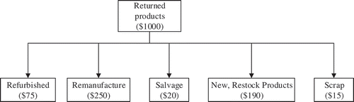
Because electronic products have short lifecycles returned products are time sensitive and any delay in remanufacturing contributes to decreasing the value of the product. For these kinds of products, the delay can be expensive as customers are less likely to buy the products that have a short life. In fact, research shows that the returned products generally lose 30% of their value in process delay (Guide et al. 2006). For example, time-sensitive electronic products like personal computers (PCs), may lose 1% of their value per week and the rate is increased at the end of the life cycle. Figure 1 shows the recovered value from returned goods by various remanufacturing processes. It can be seen that if the value of the returned items is $1000, then the buyer can only recover $550 by various reverse logistic processes, and this means that $450 is lost due to delay. After a product is sorted into distinct categories like good (reusable), moderate (remanufacture), and bad (recycle), it is crucial to perform remanufacturing operations as fast as possible. Blackburn et al. (2004), found that only 20% of the returned commodities manage to get higher value and that the remaining 80% generally drops down to the lower values.

Figure 1. Revenue generated from various remanufacturing processes, adapted from Blackburn et al. (2004).

There are two types of uncertainties related to the delay in the process: external and internal. External uncertainties take place due to variations in the quality and quantity of returned materials, changes in demand, and variations in time of product returns. Internal uncertainties incorporate accidental failures of the workstation, inappropriate buffer allocations, high congestion at the facility, and the yield rate of the entire process. The first reason for the delay in processing is the buffer allocation. Buffer capacity controls the work in process for the remanufacturing system. Proper space for work-in-process reduces the probability of ‘starvation’ and ‘blocking’ in the remanufacturing process. In starvation, the buffer is empty and the downstream machine has no parts to the process, and therefore, work must stop. Blocking is the condition in which the downstream buffer is filled to its maximum capacity, and therefore, this stops the upstream machine in discharging the finished part. Both conditions force the machines to stay idle, which creates an unnecessary delay in the process.

Another reason for work interruption is a sudden failure of the machinery. Any failure needs to be fixed by means of corrective maintenance. Corrective maintenance is a time-consuming and costly activity because the maintenance crew needs time to diagnose and repair the failed machine. In fact, increments in buffer capacity beyond the optimal level sometimes decreases the production output more than other factors. In addition, machine availability depends on its MTBF. The MTBF for any machine can be improved by introducing preventive maintenance, (PM). This policy helps to restore the reliability of a machine that has deteriorated over time. Hence, preventive maintenance is necessary to improve the availability and increase the remanufacturing rate.

To summarise, this paper will study the effect of different buffer allocations and different PM frequencies on the cycle time and profit of the remanufacturing line, which is used to remanufacture multiple products. This study will assess machines availability and buffer effectiveness. To achieve this, the current study employs a simulation-based experimental methodology to optimise the buffer allocation and PM by reducing the overall experiment size. This study tackles an important topic of research as remanufacturing industries are trying to increase their revenue by remanufacturing more products. The aim of this paper is to establish an effective way to discover the appropriate PM frequency and optimal buffer allocation so that the performance of the remanufacturing line is maximised and work is flowing without interruption or delays.

2. Literature review

Very few published works have addressed the buffer allocation issue for the remanufacturing line. But there is no consideration about the preventive maintenance and multi-product production environment. Unlike manufacturing system, remanufacturing systems are characterised by uncertain input and output patterns. The input and output patterns have uncertainty in terms of quality and quantity. Whereas both the input and the output patterns of a manufacturing system have known quality and quantity (Esmaeilian, Behdad, and Wang 2016). The role of buffer is to decouple two consecutive workstations by providing some freedom so that operations can continue in case of accidental failure and repair, as well as unequal processing times. This is true for both manufacturing and remanufacturing systems. The role of buffers may reduce/eliminate the phenomena of workstation’s blocking and starvation. Blocking phenomenon occurs when the downstream buffer is full and the upstream workstation has no place to unload its processed parts. Starvation phenomenon occurs when a downstream workstation has no parts to work on because the buffer is exhausted, and the upstream workstation is down due to failure/repair. Moreover, to alleviate uncertainty in timing and quantity of returned cores, a buffer in remanufacturing systems can be used to store returned cores or parts up to a threshold level of quantity N, above which operations resume at the workstation. This is termed as the N-policy. The remaining of this section will address models dealing with performance enhancement and buffer allocation, starting with early models dealing with a single-product setting, then presenting some of those models tackling multi-product production environment. The other two categories of the reviewed models include research works integrating the contribution of preventive maintenance, and models dealing with remanufacturing systems operating under N-policy.

Earlier work on buffer allocation in manufacturing lines relate to among others, Buzacott (1969), who presents a model for a production line composed of two stations and one buffer. Gershwin and Schor (2000), apply decomposition method for small buffers as well as small systems to produce numerical results for production rate and average buffer capacities. These models do not consider preventive maintenance since their focus is on random failure and repair. Also, they address only single-product production environment.

Many industries process multiple products. However, due to the complexity of the problem, it has only been explored in scant-published works. The issue was firstly analysed by Abdul-Kader and Gharbi (2002). Until this time, it was unacknowledged. In their study, they develop a simulation-based experimental design. The methodology was proposed to improve the performance of the manufacturing line. A nonlinear mathematical programming model was employed by Abdul-Kader, Ganjavi, and Baki (2011) to optimise the buffer capacity for a multi-product production line. They use a lexicographic goal programming method to optimise the buffer capacity. In this model, the authors did not consider explicitly the accidental failure and repair of the machines of the production line. Basically, their model is based on an ideal situation. Jarrahi and Abdul-Kader (2015), develop an analytical method to measure the performance of a multi-product unreliable production line with finite buffers between workstations. A decomposition method is then employed to approximate the production rate of the production line. A GI/G/1/N queuing model is applied to obtain parameters such as blocking and starvation probabilities that are needed for the approximation procedure. Like the earlier models, the models cited in this paragraph do not address preventive maintenance.

The reality is that cycle times are highly dependent on the buffer allocation and preventive maintenance strategy. Other literature on the production system highly concentrate on the optimal buffer inventory during the maintenance duration. Radhoui, Rezg, and Chelbi (2010) find the optimal buffer inventory, and optimal PM frequency by using experimental design. Zequeira, Prida, and Valdes (2004) define the method to find the optimal time for continuous production period and how to decide the optimal buffer inventory to satisfy demand during downtime. Zequeira, Valdes, and Berenguer (2008), with the goal of cost minimisation, use a heuristic method to find the optimal buffer size and PM frequency. Van der Duyn Schouten and Vanneste (1995), optimise the PM frequency for two machines and one buffer production line. They find the optimal way to apply the PM to improve production is by the age of the machine and its wear and tear. None of these models consider a multi-product production environment.

Similarly, Meller and Kim (1996), also calculate the effect of PM on a two-machine one buffer line. The authors address the impact of preventive maintenance on system cost and buffer size. They study a production system composed of two stations separated by an intermediate buffer where the second station is assumed reliable. The authors assume that the failure rate and repair rate of the first machine follow an exponential distribution. In their model and based on certain scenarios, it has been shown that the implementation of a preventive maintenance program decreases the system cost as well as the process variation in terms of output. Noseworthy and Abdul-Kader (2004), use a simulation-based methodology to determine the effect of periodic PM on production costs and overall production rates. Zandieh, Joreir-Ahmadi, and Fadaei-Rafsanjani (2017) propose a genetic algorithm to determine the optimal buffer allocation and period of PM. They use the normal distribution of time to represent the PM in a production line. The goal of their paper is to increase the production rate and minimise the defective rate of products and hereby minimise losses. In contrast, Nahas (2017), determines the optimal buffer allocation and rate of PM by using a decomposition method. The focus of the above-reviewed papers is on a single-product production environment.

Considering remanufacturing systems, Aksoy & Gupta, (2005), present a study to optimise buffer allocation for remanufacturing line using a heuristic algorithm. Aksoy and Gupta (2011), explore the buffer optimisation problem when servers are on break. They use a heuristic algorithm to optimise the buffer allocation. Aksoy and Gupta (2010), Su and Xu (2014), and Gu (2018) explore buffer allocation problems when servers follow N-policy. They use decomposition principle and expansion methodologies to achieve the goals of remanufacturing and hybrid production lines, respectively. Here, N-policy, means that if the quantity of returned products is less than N, then the processor or server either sits idle or continues to work on secondary work. All the literature presented for remanufacturing lines uses the reusable rate of returned product. Moreover, their models do not consider multi-product, set up times, and yield rate, which can be advantageously tackled in simulation modelling techniques given the stochastic nature of the remanufacturing operations and environment.

From the above-indicated limitations of the reviewed publications, this research paper will focus on finding the optimal buffer allocation and PM frequency with the aim to reduce cycle time and increase profit through reusing, remanufacturing, and recovering materials, which are key performance indicators in remanufacturing systems (Graham et al. 2015). Additionally, consideration of preventive maintenance and multi-product environment is integrated in this comprehensive modelling approach.

The remaining of the paper is organised as follows: Section 3 illustrates working assumptions while Section 4 describes the solution methodology. To demonstrate the applicability and usefulness of the solution approach, a case study is presented in Section 5. Finally, the conclusion and recommendations for future investigations are reported.

3. Simulation model parameters, assumptions and performance measures

This section outlines the parameters, working assumptions and performance measures used in the simulation model and experimental design.

3.1. Process parameters

The following symbols are used in this paper. The machines of the remanufacturing system are represented by M_i, where i = 1, 2 … n. The intermediate buffers are represented by B_i, where i = 1, 2 … n − 1. Products are represented by P_j, where j = 1,2 … m. During the case study, the basic parameters, which are used continuously, are as follow:

1/λ_i = Mean Time Between Failure (MTBF_i), for machine M_i

1/μ_i = Mean Time to Repair (MTTR_i), machine M_i

Z_i = maximum buffer capacity of buffer B_i

T_i = Time between PM actions

T = clock time

PM = preventive maintenance

CM = corrective maintenance

3.2. Preventive maintenance calculation

As per the study of Meller and Kim (1996), the long-run MTBF is a function of the operating time between two preventive maintenance actions and the following three parameters:

1. Current MTBF without the PM action (Minimum)

2. Maximum MTBF with very frequent PM program (Maximum)

3. β – shape factor for the asymptotic gain in PM

The user can calculate the maximum MTBF by mathematical method and approximation method. Maximum MTBF is equated by taking the availability level of 99% in Equation (1). The shape factor, β, is estimated and then the time of PM is estimated by using Equation (2).

(1) $\mathrm{C}=\frac{MTBF}{MTBF+MTTR}$(1)

(2) $\mathrm{M}\mathrm{T}\mathrm{B}\mathrm{F}=\mathrm{M}\mathrm{i}\mathrm{n}.+\left(\mathrm{M}\mathrm{a}\mathrm{x}.-\mathrm{M}\mathrm{i}\mathrm{n}.\right)(1-{{\mathrm{e}}^{-}}^{\beta /\mathrm{T}\mathrm{i}})$(2)

3.3. Performance measures

To generate the results and evaluate the serial production line, the following parameters are used in the simulation model as well as in the results.

PO = Total production output for the remanufacturing system

CT = Cycle time to finish production of one lot of each product

BZ_i = Average contents in buffer B_i

TCM_i = Total corrective maintenance time during a simulation period or

Unscheduled down time for machine M_i

TPM_i = Total PM time during a simulation period or

Scheduled downtime for machine M_i

BT_i = Total time machine M_i is blocked

3.4. Cost parameters

Various costs, like holding, corrective maintenance, and PM are calculated. All parameters used for the estimation of costs are as follows:

C_r = Cost of corrective maintenance or cost of unscheduled repair

C_p = Cost of PM or cost of scheduled repair

C_B = Operation cost of buffer

C_w = Wage of employees to operate the remanufacturing system

C_h = Inventory holding cost

C_u = Cost of utility to operate the plant

C_e = Cost of equipment and building

C_c = Cost of product collection

TC = Total cost of the remanufacturing system to operate for the defined period

The charge of the corrective maintenance, (C_r), depicts the expense to repair the machine when it fails accidentally. It consists of various fees such as labour, downtime, and maintenance. The maintenance actions that are applied to reduce the random failure of the machines incur the expenditure represented by preventive maintenance cost, (C_p). In addition, PM action includes finances related to oil changes, cleanings, inspections, labour force, and coolants. The buffer operating cost, (C_B), represents the money for storing the inventory in buffer, (Meller and Kim 1996). The inventory holding cost, (C_h), is for storing and handling the inventory in storage. The utility cost, (C_u), includes electricity and general maintenance for the plant. The cost of equipment and building, (C_e), represents the charges associated with insurance, fire protection, taxes, building rental, and machine depreciation costs; see Savaliya (2017).

(3) $\mathrm{H}\mathrm{a}\mathrm{n}\mathrm{d}\mathrm{l}\mathrm{i}\mathrm{n}\mathrm{g}\mathrm{a}\mathrm{n}\mathrm{d}\mathrm{u}\mathrm{t}\mathrm{i}\mathrm{l}\mathrm{i}\mathrm{t}\mathrm{y}\mathrm{c}\mathrm{o}\mathrm{s}\mathrm{t}=\left({\mathrm{C}}_{\mathrm{u}}+{\mathrm{C}}_{\mathrm{h}}\right)\times \mathrm{N}\mathrm{u}\mathrm{m}\mathrm{b}\mathrm{e}\mathrm{r}\mathrm{o}\mathrm{f}\mathrm{w}\mathrm{o}\mathrm{r}\mathrm{k}\mathrm{i}\mathrm{n}\mathrm{g}\mathrm{d}\mathrm{a}\mathrm{y}\mathrm{s}$(3)

(4) $\mathrm{F}\mathrm{i}\mathrm{x}\mathrm{e}\mathrm{d}\mathrm{c}\mathrm{o}\mathrm{s}\mathrm{t}=\mathrm{H}\mathrm{a}\mathrm{n}\mathrm{d}\mathrm{l}\mathrm{i}\mathrm{n}\mathrm{g}\mathrm{a}\mathrm{n}\mathrm{d}\mathrm{u}\mathrm{t}\mathrm{i}\mathrm{l}\mathrm{i}\mathrm{t}\mathrm{y}\mathrm{c}\mathrm{o}\mathrm{s}\mathrm{t}+{\mathrm{C}}_{\mathrm{e}}+\left(\mathrm{C}\mathrm{w}\times \mathrm{N}\mathrm{u}\mathrm{m}\mathrm{b}\mathrm{e}\mathrm{r}\mathrm{o}\mathrm{f}\mathrm{w}\mathrm{o}\mathrm{r}\mathrm{k}\mathrm{e}\mathrm{r}\mathrm{s}\times \mathrm{N}\mathrm{u}\mathrm{m}\mathrm{b}\mathrm{e}\mathrm{r}\mathrm{o}\mathrm{f}\mathrm{w}\mathrm{o}\mathrm{r}\mathrm{k}\mathrm{i}\mathrm{n}\mathrm{g}\mathrm{h}\mathrm{o}\mathrm{u}\mathrm{r}\mathrm{s}\right)$(4)

(5) $\mathrm{T}\mathrm{C}=\mathrm{M}\mathrm{a}\mathrm{i}\mathrm{n}\mathrm{t}\mathrm{e}\mathrm{n}\mathrm{a}\mathrm{n}\mathrm{c}\mathrm{e}\mathrm{c}\mathrm{o}\mathrm{s}\mathrm{t}+\mathrm{b}\mathrm{u}\mathrm{f}\mathrm{f}\mathrm{e}\mathrm{r}\mathrm{c}\mathrm{o}\mathrm{s}\mathrm{t}+\mathrm{f}\mathrm{i}\mathrm{x}\mathrm{e}\mathrm{d}\mathrm{c}\mathrm{o}\mathrm{s}\mathrm{t}$(5)

(6) $\mathrm{P}\mathrm{r}\mathrm{o}\mathrm{f}\mathrm{i}\mathrm{t}=\left(\mathrm{F}\mathrm{i}\mathrm{n}\mathrm{i}\mathrm{s}\mathrm{h}\mathrm{e}\mathrm{d}\mathrm{P}\mathrm{r}\mathrm{o}\mathrm{d}\mathrm{u}\mathrm{c}\mathrm{t}\mathrm{s}\times \mathrm{s}\mathrm{e}\mathrm{l}\mathrm{l}\mathrm{i}\mathrm{n}\mathrm{g}\mathrm{p}\mathrm{r}\mathrm{i}\mathrm{c}\mathrm{e}\right)-\mathrm{T}\mathrm{C}$(6)

3.5. Working assumptions

The following assumptions are considered while simulating the model of a remanufacturing system:

1. There is a continuous supply of cores to the first machine, consequently the first machine never gets starved. Accordingly, the last machine of the remanufacturing system has an infinite capacity buffer and so all remanufactured parts can exit the system easily. Hence, the last machine never gets blocked.

2. Two types of cores are remanufactured according to their lot size (the lot refers to the basic quantity). One type of the cores starts processing when the defined lot of the prior core or product finishes its production. After processing one lot of a product, a machine must be stopped to make necessary adjustments before processing another product. The processing sequence of all the products on any machine is always the same, i.e., product 1, product 2 … ., product j. For more clarity, the terms cores and products are used interchangeably in this paper.

3. All the machines of the remanufacturing system can process only one work item at a time.

4. All the transitional buffers have a finite capacity. The maximum available capacity of a buffer is Z_i.

5. All the machines are prone to unplanned breakdown. The failure rate is defined by λ_i. The random failure of a machine is usage or operation dependent. This means that if the machine is idle, then it cannot break down.

6. The transferring time of items from one machine to a buffer or from a buffer to a machine is negligible. The loading and unloading of an item onto a machine is small.

7. All the buffers are reliable. They are not subjected to random failures and repairs.

8. Corrective maintenance and PM workers are always available. Corrective maintenance is performed based on first down – first repair rule for any machine.

9. The PM frequency is predefined in the program. A machine undergoes a PM action for the expressed time scheduled.

4. Methodology

Figure 2 illustrates the flow of parts in the multi-stage remanufacturing system. The flow chart illustration follows the notation of Section 3 and shows the logic of the simulation model. In multi-stage remanufacturing lines, each part arrives in the storage. The storage has infinite capacity, and in the multiproduct production environment, all the products arrive as scheduled. As the simulation starts, first product j will move to machine 1 and at the same time, all the machines will go under the set-up downtime. When the set-up is done, a part will move to machine M₁ if the machine is available to accept the part.

Figure 2. Flow chart of simulation model.

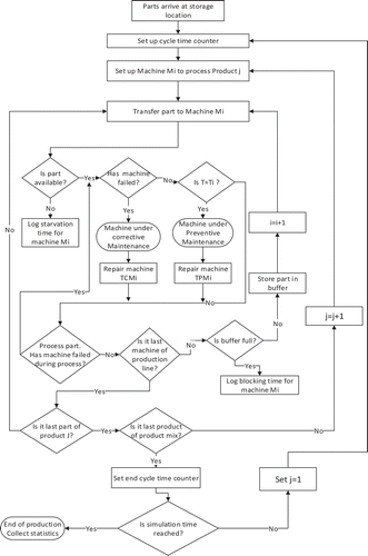
The availability of a machine depends on whether it is processing another part, or has failed, or is under preventive maintenance. If the machine is in failed condition, then the machine will be repaired by corrective maintenance and machine downtime will be noted and logged. Ideally, in good circumstances, PM is performed as per the schedule. When it is time to perform PM, there is a pause for the maintenance action to be completed, and then the machine will start processing the part. If, however, a machine fails during the processing of a part, it will be repaired and then resume the processing of the unfinished part. Normally, PM is scheduled during the simulation run.

To simplify, a part will be processed on machine M_i as soon as the machine becomes available. Once the part completes processing on machine M_i, the part is transferred to the downstream buffer if it is not full. If the buffer is full, the part will wait on the machine until a space in the buffer becomes available. At the same time, the blocking time for the machine is logged. A part will be moved out of the buffer according to the first-in-first-out (FIFO), rule and will progress to the next machine. Once a part finishes processing through all the machines, it will leave the remanufacturing line and will be placed in the inventory. If it is the last part of item j, then the simulation program will determine whether each of the components in the product mix are processed. If all the products are not processed, then it will send the next product batch to the machine and the machine will undergo the setup to process the next product, j + 1.

The set-up downtime is used to do the initial preparation for processing the new product. If it is the last part of the product mix, then the cycle time is noted for processing the batches of the product mix. When the run-time of the simulation model is reached, statistics about output results are collected and reported.

4.1. Solution approach

In a multi-product remanufacturing line, there are several factors (independent variables), which can affect the cycle time and the overall cost of the system. As the number of factors increases, the number of experiments increases as well. Thus, for longer remanufacturing lines, more experiments are needed to assess the performance of the remanufacturing system. Therefore, a mixed level fractional factorial design is considered to estimate the effect of major factors on the performance of the remanufacturing line. The ANOVA will be applied to identify the best contributing factors to the optimal performance of the remanufacturing line. The best results will be optimised further by using the Sim Runner optimiser, which is available in the software package PROMODEL, (2016). The solution approach is shown in Figure 3.

Figure 3. Solution approach.

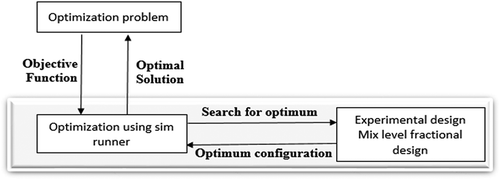
By using this solution approach, any remanufacturing line can be optimised. To optimise the remanufacturing line, an experimental design is generated, and it will be taken as an input in the simulation model. The simulation model will work as shown in Figure 2, and the results will be analysed. By statistical analysis of the results, most contributing factors will be decided. The optimal scenario from the experimental design will be identified and taken as an input in Sim Runner for further optimisation. Sim Runner will optimise the remanufacturing line parameters. Sim Runner is a built-in optimisation module in PROMODEL package, which helps to optimise the objective function within the given boundary conditions. Sim Runner works on the principle of genetic algorithm and evolutionary algorithm. The primary search process of Sim Runner is based on the evolutionary algorithm. The proposed solution approach is applied in the case study to show the usefulness of this approach.

5. Case study

5.1. Process parameters and assumptions

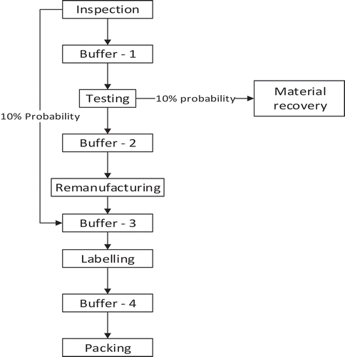
To demonstrate and validate the methodology developed in this paper, a case study is conducted on a personal computer and laptop remanufacturing line. The plant is used to remanufacture, reuse and recycle the laptops and computers. Afterwards, the same remanufacturing line is used to remanufacture both products. The flow of product in the remanufacturing line is shown in Figure 4. The returned products will pass through the inspection and testing operations. At the inspection station, some basic memory and cache tests will be done and the good-quality products will proceed to the labelling station, and the remaining products will go to the testing station. Bad-quality products will undergo material recovery operations after finishing the testing operation. The moderate quality products will go to the remanufacturing stage. In the case study, it is assumed that 10% of the products are in the good-quality category and will proceed to the labelling stations after inspection. On the other hand, 10% of the inspected products will be found to be unrepairable after the testing operation and will proceed to the material recovery operations.

Figure 4. Flow of product in computer and laptop remanufacturing line.

The processing time of the returned products highly depends on its quality and the type of problems that need to be fixed during the remanufacturing process. As a result, processing times will vary. The processing time or the exponential distribution, (e), is used to simulate the large set of possible values. The processing time for each product on each machine is shown in Table 1. As noted previously, each machine will undergo the set-up as the product changes. The set-up time is given in Table 1. All the processing times are taken from Savaliya (2017). Table 1 shows that the remanufacturing (repairing) stage has higher processing time. Hence, two remanufacturing machines in parallel are used while all the other machine stages have one machine.

Table 1. Processing times for computer and laptop remanufacturing line (taken from Savaliya (2017)).

	Set up	Inspection	Testing	Remanu-facturing	Labelling	Packing
Computer	30	e (1.23)	e (7.32)	e (20)	e (5.66)	e (9.1462)
Laptop	30	e (1.05)	e (6.5)	e (15)	e (5.66)	e (9.1462)

As indicated earlier, the machines are subject to random failures and repair. The failure and repair rates for each machine are shown in Table 2.

Table 2. Failure and repair rates.

Work station	Failure rate, λ (hours)	Repair rate, μ (hours)
Inspection	1	10
Testing	1.33	12
Remanufacturing	0.86	7.5
Labelling	0.75	6
Packing	1	8.6

The collection, labour, utility & handling, selling, and equipment costs are taken from Savaliya (2017). The holding, utility, and other fixed costs are given in Table 3. The selling price of remanufactured products is depicted in Table 3. By recycling a computer, different materials can be recovered. Therefore, the computers and laptops with the bad quality are sent for material recovery.

Table 3. Cost associated with computer and laptop.

Category of cost	Cost
Worker	$15 per hour
Utility and holding cost	$93 per day
Collection cost of computer	$150 per computer
Collection cost of laptop	$200 per laptop
Equipment cost	$811000 per year
Corrective maintenance cost	$100 per hour
Preventive maintenance cost	$10 per hour
Space cost	$0.2774 per sq. feet/hour
Selling price of computer	$250 per computer
Selling price of laptop	$400 per laptop

The recovery of computer materials can be very profitable for the firm. The value and the percentage of the recoverable materials in the computer are illustrated in Table 4.

Table 4. Recoverable materials in computer, taken from Savaliya (2017).

Material	Percent	Value ($)
Plastics	23.00	11.73
Aluminum	6.30	9.11
Steel	20.50	4.18
Gold	0.001	6.27
Silver	0.02	1.03
Lead	6.30	1.93
Cadmium	0.01	0.01
Mercury	0.0022	0.00
Total	56.13	$34.26

5.2. Preventive maintenance calculations

The failure and repair rates for each machine are indicated in Table 2. To calculate the PM frequency, Equations (1) and (2) defined in Section 3 are used. First, one needs to decide the maximum MTBF of every machine that can be achieved by the frequent PM. It is assumed that a 99% availability is achieved with PM. Consequently, the availability value is selected 99% in Equation (1) to calculate the maximum MTBF. Each machine can achieve the availability of 99% with the maximum value of the MTBF. In Table 5, simple 15 and 35-minute (or T_i), frequencies are selected to apply the PM. To estimate the value of the shape factor, β, a graph is plotted between MTBF and various shape factor values by using Equation (2) (see also Meller and Kim 1996). The estimated value of the shape factor, β, is shown in Table 5.

Table 5. Parameters of preventive maintenance.

	Inspection	Testing	Remanufacturing	Labelling	Packing
MIN.	1	1.33	0.86	0.75	1
MAX.	10	8.33	15	11.66	13.33
β	7.5	12.5	27	27	6

The parameters of Table 5 are used to find the achievable MTBF for different PM frequencies. Equation (2) calculates the achievable MTBFs for the chosen frequencies and so the achievable MTBFs are displayed in Table 6. The calculation of the MTBF for the inspection machine is given below and remaining MTBFs are calculated by using a similar method (see Equation (2), Section 3.2):

$\mathrm{M}\mathrm{T}\mathrm{B}\mathrm{F}=\mathrm{M}\mathrm{i}\mathrm{n}\left(\mathrm{M}\mathrm{T}\mathrm{B}\mathrm{F}\right)+\left(\mathrm{M}\mathrm{a}\mathrm{x}\left(\mathrm{M}\mathrm{T}\mathrm{B}\mathrm{F}\right)-\mathrm{M}\mathrm{i}\mathrm{n}\left(\mathrm{M}\mathrm{T}\mathrm{B}\mathrm{F}\right)\right)(1-{{\mathrm{e}}^{-}}^{\beta /\mathrm{T}\mathrm{i}})$

$\mathrm{M}\mathrm{T}\mathrm{B}\mathrm{F}=1+\left(10-1\right)\left(1-{\mathrm{e}}^{-7.5/15}\right)=4.54\mathrm{h}\mathrm{o}\mathrm{u}\mathrm{r}\mathrm{s}$

Table 6. MTBF and preventive maintenance frequency.

Frequency	Inspection	Testing	Remanufacturing	Labelling	Packing
N (15, 5) min	4.54	5.3	13	10	5.9
N (35, 5) min	2.7	3.4	8	6.5	2.9

In the real world, it is very hard to apply PM in the same time interval. There is always some variation in the defined frequency. The normal distribution is used in the simulation model to account for the effect of variation in PM interval. In this case study, N (15, 5) is used for 15-minute frequency, where 15 is the average time to apply PM and 5 is the standard deviation. Table 6 shows the normal distributions used in the simulation model and achievable MTBF with this time frequency.

5.3. Experimental design and analysis of the results

Experimental designs are best used to understand the effect of each factor on the remanufacturing line. Fractional factorial design is used to analyse the impact of each factor on cycle time and profit. The level of each factor for fractional design is shown in Table 7. The lower level for preventive PM is N (15, 5) minutes as we can reach the maximum MTBF with this frequency. The N (35,5) minute frequency is chosen as the higher level for the PM. The medium level will have mixed PM frequency. A machine with the highest failure rate will get the maintenance that is more frequent, and the remaining machines will get less frequent maintenance. In this case study, the inspection and packing machines have a higher failure rate. To be sure, these two machines will get PM at N (15, 5) minute intervals while the remaining machines will go under preventive maintenance at N (35, 5) minute inter vals at the intermediate levels of PM.

Table 7. Factors and their levels for experimental design.

Factor	Low	Medium	High
Buffer 1 (A)	5	10	20
Buffer 2 (B)	5	10	20
Buffer 3 (C)	5	10	20
Buffer 4 (D)	5	10	20
PM Freq. (E)	15	25	35
PM Duration(F)	1		2

By using the data of Table 7, a fractional design is modelled. Because of this, a list of 66 different scenarios is obtained to analyse the remanufacturing system. These 66 scenarios are taken as an input in the PROMODEL simulation software. From the results, the cycle time and costs are the response variables representing the performance of the system. The model is simulated for 3500 hours including a warm-up period of 700 hours and replicated 10 times. The warm-up period is determined by using Welch’s moving average method.

5.4. Analysis of variance, (ANOVA)

The results of the simulation model are inputted in the MINITAB 2016 statistical software to perform the ANOVA. At this point, ANOVA and regression analysis (variables in output), are calculated and the results of ANOVA and regression rates are shown in Tables 8 and 9.

Table 8. Analysis of variance (ANOVA).

S = 0.674210
R-Sq = 92.43%
R-Sq. (adj) = 92.12%
Source	DF	SS	MS	F	P-value
Regression	26	3511.47	135.057	297.12	0.000
Residual Error	633	287.74	0.455
Total	659	3799.21

Table 9. Coefficients of regression analysis.

Parameters	Coefficient	SE coefficient	t	P-value
Constant	60.2621	0.11689	515.548	0.000
A	1.5988	0.03610	44.290	0.000
B	1.6803	0.03692	45.508	0.000
C	−0.5732	0.03894	−14.721	0.000
D	−0.8095	0.03462	−23.384	0.000
E	−0.3299	0.03639	−9.066	0.000
F	1.1336	0.02908	38.989	0.000

The regression analysis report depicts the R² = 92.43%, which indicates a good fit of the data. In addition, Table 8 shows that the F ratio is high and equal to 297.12, and it indicates sufficient variation within sample means. The confidence interval value is 95% in the analysis of the results, and the p-value is less than 0.05 which shows the significance of the test.

Next, Table 9 shows the different coefficients of the regression analysis. The analysis indicates that buffer 3(C), buffer 4 (D) and PM frequency (E) have a positive impact on the cycle time. Buffer 4 (D) has the largest impact on the cycle time with t-statistics value of −23.384, which means that buffer 4 is significant to reduce the cycle time. Buffer 4 is followed by the buffer 3 and PM frequency with t = −14.721 and t = −9.066, respectively. The negative t-value denotes the reduction in the cycle time due to those factors. Buffer 1 (A) and buffer 2 (B) negatively affect the cycle time of the system as they have the largest positive value of the t-statistics. The value of the p-statistics is much lower than the confidence level of 5%. Therefore, we can conclude that all the factors are significant in the experiment. From the regression analysis, it is easy to see that buffer 2 and buffer 1 should have the lower capacity. Meanwhile, buffer 3, buffer 4, and the PM frequency should have higher values.

By comparing the results of the experimental design (Table 9), the best scenario was selected and optimised by using the Sim Runner and shown in Table 10. As a result, Table 10, proves that the further optimisation of the experimental design results has lowered the average cycle time. Profits for the firm has also increased with the reduction in the buffer size. Therefore, experimental designs are useful in achieving the best PM strategy and optimal buffer allocation. By following the optimal configuration obtained by using Sim Runner, the remanufacturing line can process 17,640 units of computers and laptops in a year. Out of this number, 1760 units are reused, 1580 units are recycled and remaining 14,300 units are remanufactured. Here, the profit is calculated for the overall production of the remanufacturing line. The costs are based on the number of hours of operation, they do not depend on the quantity of products. Therefore, the overall profit is generated from good and moderate quality products.

Table 10. Optimized results for remanufacturing line.

Result type	A	B	C	D	E	F	Cycle time (hours)	Profit ($)
Experimental design	5	5	5	20	25	1	56.53	288,817
Sim Runner	1	4	5	20	25	1	55.19	316,948

5.5. Revenue generated by recycling products

Table 10 demonstrates the optimal results by Sim Runner, and it generates the maximum production. The recycled quantity is selected from the best scenario of Sim Runner to calculate the revenue. Once units are recycled, valuable materials such as gold, silver, and platinum can be recovered. The metal present in a regular computer is given in Table 4. By recycling a computer or laptop, factory owners can generate an average revenue of $34.26. Table 11, (below), displays the recycled quantity of each product and the total revenue for the firm. This can generate about $54,000 of revenue by recycling a total of 1,580 computers/laptops. Accordingly, instead of consumers throwing their electronic products away, they should be encouraged/motivated to recycle the material and this, in turn, can be very profitable for a company wishing to use those parts. In this way, natural resources can be preserved while pollution and energy consumption can also be reduced.

Table 11. Revenue generated by recycling computers and laptops.

Computer (units)	Laptops (units)	Revenue ($)
886	694	~$54,130.00

5.6. Factors analysis and optimisation

The analysis of factors is accomplished by two methods. The first method is to perform the ANOVA on the results of the experimental design and then determine the factors with the greatest impact on the response variable. For instance, Table 9 shows that buffer 2, buffer 4, and PM have the greatest impact on the dependent variable. This data is enough to decide the optimal range of factors, and these factors should be further optimised using Sim Runner. This is an efficient way to reduce the experiment size and optimise the results.

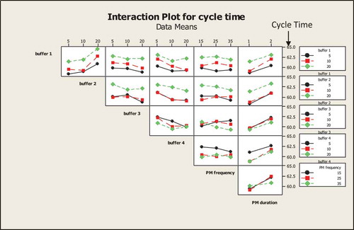
On the other hand, the second method of considering data is to examine the interaction plot between the factors and then analyte the effect of each one. For example, Figure 5 shows the interaction plot between the factors and the cycle time. In other words, the interaction plot shows that if buffer 1 and buffer 2 have higher capacities than the remanufacturing line will have the maximum cycle time (less production). This graph clearly depicts that a PM strategy has the lowest cycle time when the duration of PM is short. The graph illustrates that buffer 4 has a bigger impact over buffer 3. It also shows that if buffer 4 has the higher value, then we can achieve the lower cycle time by keeping buffer 3 at the lower level. It follows then that buffer 1 and buffer 2 increase the cycle time with higher capacity. Therefore, it is necessary to keep buffer 1 and buffer 2 at lower levels. The interaction of PM frequency and buffer 3 shows that if buffer 3 has a smaller capacity then it minimises the cycle time. The factor Duration of PM always increases the cycle time. Thus, it is necessary to accomplish the PM action in small durations. After analysing the interaction plot of the second method, it can be concluded that buffer 1, buffer 2, and buffer 3, should be held at lower levels to achieve the minimum cycle time.

Figure 5. Interaction plot for cycle time.

5.7. Preventive maintenance analysis

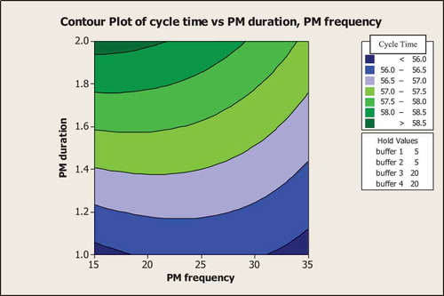
There is no mistaking that PM is a very critical factor in the remanufacturing line to reduce accidental failure. It is worth emphasising again that different PM frequencies are useful to achieve the maximum MTBF. The choice of the best PM frequency is essential to reduce the accidental failure of the machines and subsequent delays without affecting or reducing production output (PO). Moreover, the duration of the PM also affects the cycle time. These points must be clearly established so that the relationship between different PM frequencies and PM durations is understood. Figure 6 represents the relationship between different frequencies of PM and the duration of PM when all the buffers are kept at optimal values. From the graph below, PM frequency shows significant variation in the cycle time with optimal values of the buffer. Figure 6 clearly depicts that as the duration of PM increases, then only 35-minute frequency is necessary to achieve the optimal cycle time. Other frequencies increase the cycle time with increments in duration of PM. Nevertheless, the best results are noticed with even moderate levels of PM. Hence, PM frequency does not only depend on the duration of the PM, but it also depends on the duration of the corrective maintenance.

Figure 6. Contour plot of cycle time.

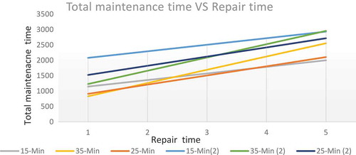
To continue, Figure 7 depicts the relationship between total maintenance time and repair time. It shows the best frequency to apply PM is when there are different durations of PM and CM. Similarly, to PM, when machine downtime decreases in CM, it also improves the output of the system. Here x-axis denotes the repair time. Moving in the right-side direction on the x-axis, the value shows the increment in repair time. If the repair time is doubled, then it is represented by 2. If, however, the repair time is 3 times more than the original repair time then it is represented by 3 on the X-axis. To go on, Y-axis denotes the total maintenance time for the remanufacturing line. The graph is plotted for three different frequencies, which are mentioned in this case study. After analysing the graph, it is obvious that if PM and CM durations are small, then the manager can use less frequent or failure-based PM. If both durations are high, then the overseer can use a moderate level frequency as mentioned in this case study because it has the least total maintenance time. If CM duration is high and PM duration is small, then a simple 15-minute frequency can be used to minimise the total maintenance time. If the PM is high and the CM duration is small, then managers can use less frequent PM to get a higher production output by reducing maintenance time.

Figure 7. Total maintenance time vs repair time.

The duration of CM affects the availability of the machine, which can be represented by Equation (1) (see Section 3.2), where C is the long-term availability of the machine. From Equation (1), it is plain that any increase in MTTR decreases the availability of the machine. The reduction in availability reduces the uptime of the machine and production output. Thus, not only PM duration but CM duration also has a noticeable role in determining optimal PM frequency. If all machines have different failure rates, then it is better to perform PM on individual machines consistently so the remaining machines may continue to work well from the buffer inventory during that period. This will increase the availability of all the machines and improve the production rate. If, on the contrary, all the machines have similar failure rates, then the manager can perform PM on the whole remanufacturing line at the same time to minimise maintenance time. Overall, the failure rate, repair rate, and duration of PM, should be considered from the start to get the ideal frequency of PM.

6. Conclusion

This paper addresses the problem of unreliable remanufacturing systems with the purpose of improving performance and reducing or eliminating potential delays that may occur due to accidental failure of equipment. This research also wishes to contribute in the implementing of a more viable pricing policy for remanufactured products. Parameters such as PM duration and frequency, the accidental failure and repair of remanufacturing equipment and buffer allocation, have been considered at length. A simulation-based experimental methodology has been presented to optimise the buffer capacity and frequency of PM, with the aim of improving the cycle time of a remanufacturing line. This methodology has been demonstrated by considering a facility that is remanufacturing desktop and laptop computers. The experimental design of the variables has helped to determine the impact of different buffer sizes on the whole cycle time. The results obtained by simulation have been further optimised by using Sim Runner. This solution approach of experimental design and optimisation reduced the overall experiment size. This greatly helps managers obtain the best performance measures within the least amount of time. The results as presented using contour and interactions plots are expressive in terms of reducing the cycle time, increasing the profit, sizing the capacity of each buffer, and determining the best PM duration and frequency. Regression and ANOVA tables show a very good fit of the results. These contribute to a better decision-making process and provide managerial insights.

For future work, those in leadership can focus on optimising the number of workers needed for the task. Furthermore, future research can focus on how PM frequency affects the defective rate of machines and tools that do not operate properly as well as the set-up time. There is no doubt that the MTBF of any machine changes with the change in PM frequency and that any change in the MTBF affects the quality of the work piece (Koren, Hu, and Weber 1998) and set up time of the machines. Without question, this MTBF relationship can and should perform a vital role in order to achieve the highest production rates at the lowest costs.

Acknowledgment

The authors are very grateful to the anonymous reviewers for their constructive comments that improved the manuscript. Our sincere thanks are addressed to the Editor for his guidance through the review process of the manuscript. The authors would like to acknowledge the financial support received during the tenure of this research work from the Natural Sciences and Engineering Research Council (NSERC) of Canada.

Disclosure statement

No potential conflict of interest was reported by the authors.

Additional information

Notes on contributors

Ronak Savaliya

Ronak Savaliya is currently working as Manufacturing engineer at Linamar Corporation, Ontario, Canada. He has completed his Bachelor of Engineering in Mechanical Engineering from Gujarat Technological University, Gujarat, India. He also holds master’s degree in Mechanical Engineering from University of Windsor. His research areas are performance optimization, preventive maintenance, and process optimization of remanufacturing systems.

Walid Abdul-Kader

Walid Abdul-Kaderis a professor of Industrial Engineering in the Faculty of Engineering at the University of Windsor, Windsor, Canada. He holds a PhD degree in Mechanical Engineering from Université Laval, Québec City, Canada. He completed his bachelor’s degree from Université du Québec à Trois-Rivières, Canada, and master’s degree from École polytechnique de Montréal, Canada. His research interests relate to performance evaluation of reverse logistics and manufacturing/remanufacturing systems prone to accidental failure and repair. His publications have appeared in many leading national and international journals and conferences proceedings.

References

- Abdul-Kader, W., O. Ganjavi, and F. Baki. 2011. “A Nonlinear Model for Optimizing the Performance of A Multi-Product Production Line.” International Transactions in Operational Research 18 (5): 561–577. doi:10.1111/j.1475-3995.2011.00814.x.
- Abdul-Kader, W., and A. Gharbi. 2002. “Capacity Estimation of a Multi-Product Unreliable Production Line.” International Journal of Production Research 40 (18): 4815–4834. doi:10.1080/0020754021000024148.
- Aksoy, H. K., and S. M. Gupta. 2005. “Buffer Allocation Plan for a Remanufacturing Cell.” Computers and Industrial Engineering 48 (3): 657–677. doi:10.1016/j.cie.2003.03.007.
- Aksoy, H. K., and S. M. Gupta. 2010. “Near Optimal Buffer Allocation in Remanufacturing Systems with N-Policy.” Computers and Industrial Engineering 59 (4): 496–508. doi:10.1016/j.cie.2010.06.004.
- Aksoy, H. K., and S. M. Gupta. 2011. “Optimal Management of Remanufacturing Systems with Server Vacations.” International Journal of Advanced Manufacturing Technology 54 (9–12): 1199–1218. doi:10.1007/s00170-010-3001-z.
- Blackburn, J. D., V. D. R. Guide, G. C. Souza, and L. N. Van Wassenhove. 2004. “Reverse Supply Chains for Commercial Returns.” California Management Review 46 (2): 6–22. doi:10.2307/41166207.
- Buzacott, J. A. 1969. “Methods of Reliability Analysis of Production Systems Subject to Breakdowns.” In Operations Research Proceedings of NATO Conference, Turin, Italy, June 24–July 4, edited by D. Grouchko, 211–232. London: Gordon and Breach Science Publishers.
- Esmaeilian, B., S. Behdad, and B. Wang. 2016. “The Evolution and Future of Manufacturing: A Review.” Journal of Manufacturing Systems 39: 79–100. doi:10.1016/j.jmsy.2016.03.001.
- Gershwin, S. B., and J. E. Schor. 2000. “Efficient Algorithms for Buffer Space Allocation.” Annals of Operations Research 93 (1–4): 117–144. doi:10.1023/A:1018988226612.
- Graham, I., P. Goodall, Y. Peng, C. Palmer, A. West, P. Conway, J. E. Mascolo, and F. U. Dettmer. 2015. “Performance Measurement and KPIs for Remanufacturing.” Journal of Remanufacturing 5 (10): 1–17. doi:10.1186/s13243-015-0019–2.
- Gu, F. (2018). “Performance Improvement of Remanufacturing Systems Operating under N-Policy” (Master’s thesis), University of Windsor, Canada
- Guide, V. D. R., G. C. Souza, L. N. Van Wassenhove, and J. D. Blackburn. 2006. “Time Value of Commercial Product Returns.” Management Science 52 (8): 1200–1214. doi:10.1287/mnsc.1060.0522.
- Jarrahi, F., and W. Abdul-Kader. 2015. “Performance Evaluation of a Multi-Product Production Line: An Approximation Method.” Applied Mathematical Modelling 39 (13): 3619–3636. doi:10.1016/j.apm.2014.11.059.
- Koren, Y., S. J. Hu, and T. W. Weber. 1998. “Impact of Manufacturing System Configuration on Performance.” CIRP Annals-Manufacturing Technology 47 (1): 369–372. doi:10.1016/S0007-8506(07)62853-4.
- Meller, R. D., and D. S. Kim. 1996. “The Impact of Preventive Maintenance on System Cost and Buffer Size.” European Journal of Operational Research 95: 577–591. doi:10.1016/0377-2217(95)00313-4.
- Nahas, N. 2017. “Buffer Allocation and Preventive Maintenance Optimization in Unreliable Production Lines.” Journal of Intelligent Manufacturing 28 (1): 85–93. doi:10.1007/s10845-014-0963-y.
- Noseworthy, S., and W. Abdul-Kader. 2004. “Impact of Preventive Maintenance on Serial Production Line Performance: A Simulation Approach.” Proceedings of the Administrative Sciences Association of Canada, ASAC 2004 Conference, Production and Operations Management Division, Quebec City, Canada.
- Radhoui, M., N. Rezg, and A. Chelbi. 2010. “Joint Quality Control and Preventive Maintenance Strategy for Imperfect Production Processes.” Journal of Intelligent Manufacturing 21 (2): 205–212. doi:10.1007/s10845-008-0198-z.
- Ravi, V., R. Shankar, and M. K. Tiwari. 2005. “Analyzing Alternatives in Reverse Logistics for End-Of-Life Computers: ANP and Balanced Scorecard Approach.” Computers & Industrial Engineering 48 (2): 327–356. doi:10.1016/j.cie.2005.01.017.
- Savaliya, R. (2017). “Performance Evaluation of Remanufacturing Systems” (Master’s thesis), University of Windsor, Canada
- Su, C., and A. Xu. 2014. “Buffer Allocation for Hybrid Manufacturing/Remanufacturing System considering Quality Grading.” International Journal of Production Research 52 (5): 1269–1284. doi:10.1080/00207543.2013.828165.
- Van der Duyn Schouten, F. A., and S. G. Vanneste. 1995. “Maintenance Optimization of a Production System with Buffer Capacity.” European Journal of Operational Research 82 (2): 323–338. doi:10.1016/0377-2217(94)00267-G.
- Zandieh, M., M. N. Joreir-Ahmadi, and A. Fadaei-Rafsanjani. 2017. “Buffer Allocation Problem and Preventive Maintenance Planning in Non-Homogenous Unreliable Production Lines.” The International Journal of Advanced Manufacturing Technology. doi:10.1007/s00170-016-9744-4.
- Zequeira, R. I., B. Prida, and J. E. Valdes. 2004. “Optimal Buffer Inventory and Preventive Maintenance for an Imperfect Production Process.” International Journal of Production Research 42 (5): 959–974. doi:10.1080/00207540310001631610.
- Zequeira, R. I., J. E. Valdes, and C. Berenguer. 2008. “Optimal Buffer Inventory and Opportunistic Preventive Maintenance under Random Production Capacity Availability.” International Journal of Production Economics 111 (2): 686–696. doi:10.1016/j.ijpe.2007.02.037.