A complex filter-based adaptive integral grid synchronisation algorithm for a PV system

ABSTRACT

The issues such as deterioration of power quality owing to nonlinear loads, sudden changes in load demand, switch to dynamic loads, the occurrence of fault at the load or grid side is addressed using proposed DQ frame Complex Filter-based Adaptive Integral Algorithm (DCFAIA). The objective of the proposed control algorithm is to maintain the frequency at the desired level irrespective of electrical disturbances and also to remove the DC offset present in the synchronising parameters due to nonlinear load, lower the harmonic content in the grid parameters and maintain the power factor unity by compensating the reactive power. The performance of the proposed algorithm is compared with that of conventional algorithms such as Improved Second-Order Generalised Integrator (ISOGI), Third Order Generalised Integrator (TOGI), Least Mean Fourth (LMF). From the comparative assessment, it is observed that the proposed algorithm exhibits superior performance in terms of precision, settling time, steady and transient errors.

KEYWORDS:

• Photovoltaic
• complex filter
• integral algorithm
• total harmonic distortion
• delayed signal cancellation

Introduction

The trend of global energy scenario based on policies been introduced in recent past and usability of electricity shows the increase in energy demand by more than a quarter by the end of 2040. The biggest challenge is to meet the energy demand without sacrificing the climate target of reducing CO₂ emission to approximately 20 Gigatonne from 37.15 Gigatonne as of now globally by introducing new sustainable development policies reported in Bridge et al. (2018). The strategy to achieve climate target indicates the replacement of high carbon emission sources with that of low carbon emission sources such as PV and wind energy sources for power generation. Many control issues are encountered in synchronising a PV system to a utility grid, e.g. sudden changes in loads, power quality issues owing to nonlinear loads and variation in solar insolation.

To address these aforementioned issues, a lot of research has been directed in structuring and executing advanced control algorithms to improve the quality of power flow in the tie line. Various techniques (Salas et al. 2006) have already been proposed to model the solar Photovoltaic (PV) system and to track maximum power from solar irradiance effectively and efficiently. The methods such as incremental conductance (IC), Perturb & Observe (P&O) technique, estimated perturb-perturb technique, Incremental Conductance with Integral Regulator (ICIR)(Subudhi and Pradhan 2013; Choudhury, Dash, and Sharma 2019), hybrid Maximum Power Point Tracking (MPPT) techniques (Rout et al. 2014) are widely used to extract maximum power from solar PV system. Taking benefits like efficiency, cost-effective, lossless, and ease of implementation into account, the single-stage PV connected system (Libo, Zhengming, and Jianzheng 2007; Swain and Subudhi 2017) is considered.

The utility system mainly disturbed due to use of nonlinear loads, unbalanced loads, and interfacing of solid-state devices, sudden switching of dynamic loads, symmetrical, and unsymmetrical faults. It is necessary to maintain the stability of the overall system complying with the grid codes and to improve the performance of the overall system ensuring the qualitative flow of power to the grid. To achieve these objectives many control algorithms have been proposed in the literature. Field oriented vector control technique is addressed in Blaabjerg et al. (2006). The objective of this technique is to maintain the reactive power at the zero levels which in turn makes the power factor unity. It is using Synchronous Reference Frame Phase Locked Loop (SRFPLL) technique to determine the angle of orientation to estimate DQ components in adverse as well as in normal conditions. Nevertheless, it is noticed that the dynamic response of such systems is poor in adverse conditions and also lacks in mitigating selective harmonics. To improve the performance of the aforementioned controller, a pre-filtering stage (Li et al. 2014) is added with SRFPLL to estimate the fundamental phase and frequency. In Mojiri, Karimi-Ghartemani, and Bakhshai (2007), an adaptive notch filter is added along with Phase Locked Loop (PLL) at the pre-filtering stage to remove selective harmonics in certain conditions. An Improved linear sinusoidal tracer-based control scheme focuses on faster convergence rate but endures poor-forced responses (Singh, Jain, and Goel 2014), similarly LMF (Walach and Widrow 1984), De-correlation Normalised Least Mean Square (DNLMS) (Pradhan et al. 2018) have also proposed fast convergence algorithm for improving the performance of the utility system. The above-mentioned algorithms are employing adaptive filters to reduce impulsive noise through the weight-updating process with reduced computation. In Variable Step Size Least Mean Square (VSSLMS) (Beniwal, Hussain, and Singh 2017), a variable step size is used to achieve the better accuracy in dynamic performance.

To improve the steady and dynamic capability of Grid Integrated PV System (GIPVS) second-order generalised integrator (SOGI) based algorithms have been proposed by many researchers. These algorithms have poor frequency adaptability capacity; hence the adaptability is improved by adding Frequency Locked Loop (FLL) with SOGI-based algorithms (Shah, Hussain, and Singh 2019). SOGI-FLL algorithms have better capability to reject DC offset and selective harmonics as compared to other algorithms which do not use FLL. To achieve better adaptability capability to reject uncertainty addition of lead compensator along with PLL is suggested in Freijedo et al. (2011) and Golestan et al. (2015). It has been found from the above literature that using effective pre-filtration stage along with PLL a GIPVS can work effectively in adverse grid conditions. The proposed grid integrated PV system comprises the following stages, namely, pre-filtering, Delayed Signal Cancellation Phase Locked Loop (DSCPLL) and adaptive generalised integrator. In pre-filtering stage, a stationary frame Complex filter (SFCF) is designed to disseminate positive and negative sequence frequencies since it has an advantage to make asymmetrical frequency response zero. SFCF has also the capability to reject DC offset. In the second stage, a synchronous reference frame delayed signal cancellation PLL (Wang and Li 2011) is introduced to cancel the selective harmonics by choosing appropriate controlled parameter. In this stage, the fundamental frequency is also estimated for different test cases which are discussed in further sections of this article. In the third stage, an adaptive generalised integrator is used to estimate the required reference grid current to improve the performance of overall system.

The overall behaviour of the PV integrated Grid system is analysed for different abnormalities and the stability of the control algorithm is analysed based on Mean Square Deviation (MSD). The objectives of the paper are as follows:

• The active and reactive components of the load current are estimated using DCFAIA.

• The fundamental frequency is estimated under adverse grid conditions.

• ICIR-based MPPT technique is used to extract maximum power for variation in solar temperature and irradiance.

• DC offset is rejected using a properly controlled parameter.

• Selective harmonic components are wiped out by setting proper parameters of DSCPLL.

In this paper, a DCFAIA-based PV-Grid synchronising control scheme is proposed to satisfy the aforementioned objectives. Different cases are considered to evaluate the performance of the proposed algorithm. A comparative analysis is made between an existing controller and the proposed control algorithm. The contributions of the paper are as follows:

• Modified PLL technique is used to handle steady and dynamic abnormalities which are not able to address generally by standard PLL technique.

• The advantages of complex coefficient filter and the cascaded-delayed signal cancellation are taken into consideration for forming a hybrid pre-filtration stage for PLL.

• Generally, in SOGI or SOGI-FLL based algorithms, many researchers have used the constant frequency for estimation of active and reactive component of load current. It has found that the actual input frequency is perturbed when the grid is subject to different types of non-linearities. The change in frequency value affects the integral gain of the SOGI-based controller and it leads to the poor estimation of DQ component of load current. So, it is necessary to make the integral gain adaptive to address the aforesaid issues. To do so the frequency is made adaptive by proposed PLL for better estimation of in-phase and quadrature component of load current.

• The proposed algorithm is tested in a single-phase grid integrated PV system using LabVIEW through the data acquisition process.

The paper is organised as follows. Section 2 describes the modelling of PV-Grid System where the detail modelling of the overall system along with the calculation of required system parameters is discussed. The mathematical analysis of the proposed DCFAIA-based control scheme and the stability analysis of the proposed method is explained in Section 3. The simulation results are discussed in Section 4, whereas the experimental analysis is given in Section 5, the brief conclusion is presented in Section 6, and the list of abbreviations are given in Appendix-II.

PV-Grid integrated system

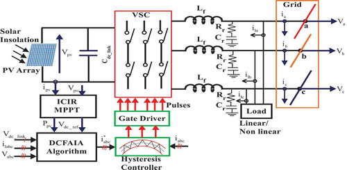
The topology of the PV-Grid integrated system is shown in Figure 1. The overall system is modelled using MATLAB/SIMULINK. It consists of a 10kW PV array tied with the utility grid through a Voltage Source Converter (VSC). The VSC is fed through a DC-link capacitor, where it is required to maintain the voltage constant irrespective of the abnormalities. ICIR MPPT controller is employed to maintain the constant input voltage across DC-link capacitor and extract maximum power from the PV array under different irradiances. Along with the ICIR MPPT scheme, a DCFAIA controller is purposefully employed to eradicate disturbances happen due to grid as well as PV side and maintain the grid as well as source parameter intact. The detailed analysis of the proposed controller is given in the following section. The parameters required for the integration of PV with the utility grid are given in Appendix–I.

Figure 1. Topology of PV-Grid Integration System.

MPPT- and DCFAIA-based control scheme

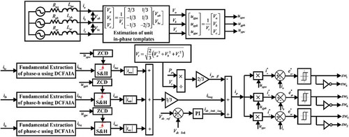
The proposed PV-grid synchronising control scheme comprises an incremental conductance Integral regulator MPPT controller for extracting maximum power from the PV set up followed by the estimation of the DC-link reference voltage by employing the DCFAIA algorithm. The DC-link reference voltage is then compared with the actual voltage obtained across the DC-link capacitor and the error is fed to the PI controller to calculate the DC power loss component. This loss component is further used by DCFAIA along with the AC loss component to estimate the active weights. The active weights are used in the following section to estimate the reference grid current (i_a*, i_b*, i_c*). The reference grid current is compared with the actual grid current sensed at the PCC using a comparator to obtain the desired error. The error is then passed through hysteresis band of width 0.01 to obtain required pulses for the controlled solid-state switches of VSC to synchronise the PV system with the existing grid effectively in adverse conditions. The overall structure of DCFAIA control scheme is shown in Figure 2. The control structure consists of the following blocks to execute aforesaid functions:

• ICIR MPPT Controller;

• Fundamental extraction of load current;

• Estimation of reference grid current;

• Generation of switching pulses using hysteresis controller.

The functionality of each block is explained in the following subsections.

Figure 2. Detail Structure of DCFAIA Control Scheme.

3.1. ICIR MPPT controller

An incremental conductance-based MPPT algorithm is used for extracting maximum power from PV array and also it is maintaining the DC-link reference voltage constant. Maximum power is attained when:

(1) $\frac{d{P}_{pv}}{d{V}_{pv}}=0\Rightarrow \frac{i_{pv}}{V_{pv}}+\frac{d{i}_{pv}}{d{V}_{pv}}=0$(1)

Figure 3 shows the P_pv versus V_pv characteristic, where three operating points, namely (A, B, and C) are mentioned to demonstrate the variation of V_pv with a change in (dP_pv/dV_pv).

Figure 3. P_pv -V_pv characteristic showing increment and decrement of V_pv.

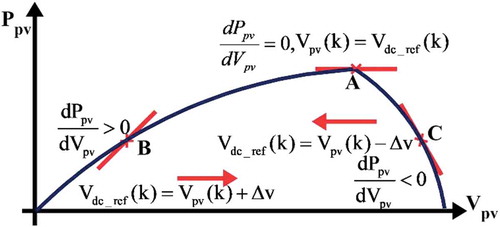
The following observations about conductance (i_pv/V_pv) and incremental conductance (di_pv/dV_pv) are made from Figure 3.

(2) $\left.\begin{array}{c}\frac{d{P}_{pv}}{d{V}_{pv}}=0\Rightarrow \frac{d{i}_{pv}}{d{V}_{pv}}=-\frac{i_{pv}}{V_{pv}},V_{pv}=V_{dc\mathrm{\_}ref}\\ \frac{d{P}_{pv}}{d{V}_{pv}}>0\Rightarrow \frac{d{i}_{pv}}{d{V}_{pv}}>-\frac{i_{pv}}{V_{pv}},V_{pv}<V_{dc\mathrm{\_}ref}\\ \frac{d{P}_{pv}}{d{V}_{pv}}<0\Rightarrow \frac{d{i}_{pv}}{d{V}_{pv}}<-\frac{i_{pv}}{V_{pv}},V_{pv}>V_{dc\mathrm{\_}ref}\end{array}\right\}$(2)

To maintain the voltage across the PV array at its reference value, a small change in voltage (∆v) is either added or subtracted from V_pv depending upon the condition stated in Equation 2(2) $\left.\begin{array}{c}\frac{d{P}_{pv}}{d{V}_{pv}}=0\Rightarrow \frac{d{i}_{pv}}{d{V}_{pv}}=-\frac{i_{pv}}{V_{pv}},V_{pv}=V_{dc\mathrm{\_}ref}\\ \frac{d{P}_{pv}}{d{V}_{pv}}>0\Rightarrow \frac{d{i}_{pv}}{d{V}_{pv}}>-\frac{i_{pv}}{V_{pv}},V_{pv}<V_{dc\mathrm{\_}ref}\\ \frac{d{P}_{pv}}{d{V}_{pv}}<0\Rightarrow \frac{d{i}_{pv}}{d{V}_{pv}}<-\frac{i_{pv}}{V_{pv}},V_{pv}>V_{dc\mathrm{\_}ref}\end{array}\right\}$(2) . An integral regulator (IR) is used along with IC to minimise the error shown in the left-hand side of the Equation 1(1) $\frac{d{P}_{pv}}{d{V}_{pv}}=0\Rightarrow \frac{i_{pv}}{V_{pv}}+\frac{d{i}_{pv}}{d{V}_{pv}}=0$(1) . This method is advantageous than P&O in terms of decent yielding under quickly changing atmospheric conditions.

3.2. Fundamental extraction of load current using DCFAIA

Figure 4. Structure showing fundamental extraction of i_a using DCFAIA.

It is necessary to comply with the grid codes expressed in an earlier section irrespective of unsettling disturbances happens at the source and sink in GIPVS. The grid is always disturbed due to the end-user consumption, which is technically called as load. This may be linear or nonlinear in nature.

The excess use of active loads affects the phase and frequency of the grid voltage which in turn affects the active and reactive power flow from source to sink. The most essential detract from the above articulations is to make the load current distortion free. The block diagram representation of the fundamental extraction from the distorted load current using DCFAIA control scheme is shown in Figure 4. The control scheme uses two major components namely, DSCPLL and an Adaptive Generalised Integrator (AGI) to extract the fundamental components.

Figure 5. Basic Structure of Stationary Frame Complex Filter.

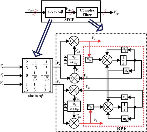
DSCPLL is the major element for the extraction of the fundamental component corresponding to changes in phase, frequency, and amplitude of the grid voltage under abnormal conditions. The objective of the PLL scheme is to estimate the frequency required for the updation of coefficients of the AGI. In actual grid integration scenario, the utility voltage is non-sinusoidal yet contorted by different external factors such as signal and power conversion errors, non-linearity sink, and the insertion of measurement devices, which outcomes in phase jump, change in nominal frequency, harmonics, and offset. It is also observed that the error in phase angle perturbs the utility frequency which in succession makes the amplitude of the fundamental component erroneous. To obtain the error-free extraction satisfying the stability criteria, it is essential to reduce the frequency error and intact the frequency at its nominal value using DSCPLL.

The proposed PLL has two stages of operation. In the first stage, a pre-filter namely SFCF (Li et al. 2014) is used, which enables to make refinement among fundamental frequency positive and negative sequence components and also attenuates the harmonics to a certain level using the cut-off frequency of complex band pass filter. The basic structure of SFCF is shown in Figure 5. In this method, the stationary frame fundamental component is estimated using a BPF with centre at natural fundamental grid frequency.

Figure 6. Bode Magnitude plot of Band Pass Filter and Complex Filter.

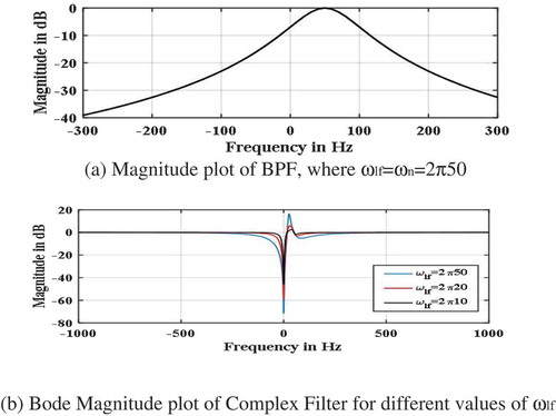
The frequency versus magnitude plot is drawn to display the characteristics of BPF which is used as a prime component in SFCF. Figure 6a shows, the BPF only allows the fundamental frequency components and lessens other frequency components. Bode magnitude plot of Complex Filter is shown in Figure 6b. It may be seen from Figure 6b that SFCF obstructs the dc part and passes fundamental frequency components.

In the second phase of activity, a DSC block is used alongside SFCF to improve the performance of PLL under the negating grid condition. The block helps to attenuate the dc component as well as some of the selective harmonic components. The value of n_eq in Equation 11(11) $n_{eq}=\sum _{j=1}^m\frac{1}{n_j}$(11) decides the order of harmonics to be eliminated. In this DSC n1, n2, n3, n4 are chosen as 2,4,8,16, respectively. So according to Equation 11(11) $n_{eq}=\sum _{j=1}^m\frac{1}{n_j}$(11) , $n_{eq}=\frac{1}{2}+\frac{1}{4}+\frac{1}{8}+\frac{1}{16}=\frac{15}{16}=0.9375$, hence $T_d=\frac{0.9375}{2\times 50}\simeq 9.4ms$. Substituting n1, n2, n3, and n4 separately in Equation 12(12) $n_j=\left|\frac{h}{2i\pm \frac{1}{2}}\right|,where\stackrel{\hspace{0.17em}}{\hspace{0.17em}}i=0,1,\mathrm{2....}$(12) , it is observed that in DQ reference frame $h=\pm 1,\pm 2,\pm 3,\pm \mathrm{4.....}\pm 15,\pm 17,\pm 18,\pm \mathrm{19...}$ and in abc frame $h=0,-1,\pm 2,\pm \mathrm{3.....}+15,\pm 16,-17,\pm 18,\pm \mathrm{19...}$ will be eliminated following the relationship given in Equation 3(3) ${\overrightarrow{V_{abc}}}^h={\overrightarrow{V_{dq}}}^{h-1}$(3) .

(3) ${\overrightarrow{V_{abc}}}^h={\overrightarrow{V_{dq}}}^{h-1}$(3)

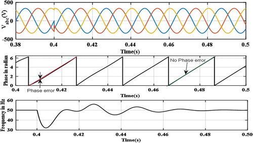
To verify the effectiveness of DSCPLL, the response of phase error (∆θ) with a phase jump of −40◦ is shown in Figure 7, where the values of ω₀, K_p, and K_i are chosen as 2π10, 88.86, and 3948, respectively. A phase change is introduced at 0.4 s as shown in Figure 7. It is observed that irrespective of phase change of – 40◦, the estimated frequency settles to its nominal value within approximately 50 ms which means that faster dynamic response is achieved.

Figure 7. Response of V_abc, phase, and frequency with a phase jump of – 40◦.

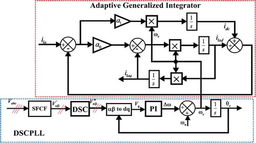
A third-order generalised integrator algorithm is taken into consideration for the estimation of active and reactive weights which further be responsible for generating effective reference currents. AGI estimates the in-phase and quadrature component of load current for three phases. The estimation of a- phase load current using AGI is shown in Figure 4. The input load current (i_la) is separated from unwanted selective harmonics and quadrature move from the fundamental component (i_laq) of load current is the yield of AGI algorithm. The closed-loop transfer function (CLTF) corresponding to i_laq is given in Equation 19(19) $\frac{I_{laq}\left(s\right)}{I_{la}\left(s\right)}=\frac{{\alpha }_0{\omega }_e^{2}s}{s^3+{\omega }_e\left({\alpha }_0+{\alpha }_1\right)s^2+{\omega }_e^{2}s+{\alpha }_1{\omega }_e^3}$(19) . From the CLTF, the characteristic polynomial F(s) is found to be s³ + (α₀ + α₁) ω_es² + ω²s + α₁ω³ = 0, where ω_e is the estimated frequency, α₀ = 2ξ and α₁ = 0.25ξ are the characteristic parameter (Vedantham et al. 2017) of AGI. The value of α₀ and α₁ should be greater than zero for a stable system. Detail mathematical analysis of the DCFAIA control scheme and its functionality are explained in the following section.

3.3. Mathematical analysis of DCFAIA

The structure shown in Figure 4 contains SFCF, DSC along with PI controller to estimate the frequency required for AGI. The mathematical procedure to obtain the required frequency and to eliminate the DC offset, harmonics are explained.

The three-phase voltage V_abc is converted to Vαβ using Equation 4(4) $V_{\alpha }+j{V}_{\beta }=\frac{2}{3}\left(V_a+V_b\cdot e^{j2\pi /3}+V_c\cdot e^{-j2\pi /3}\right)$(4) .

(4) $V_{\alpha }+j{V}_{\beta }=\frac{2}{3}\left(V_a+V_b\cdot e^{j2\pi /3}+V_c\cdot e^{-j2\pi /3}\right)$(4)

The fundamental frequency positive sequence component ($V_{\alpha \beta }^{\prime }$) is estimated using a Low pass filter (LPF) and a Band Pass Filter (BPF).

(5) $\begin{array}{c}{V^{\prime }}_{\alpha }=V_{\alpha }-V_{\alpha 3}=V_{\alpha }-V_{\alpha 2}\left(\frac{{\omega }_{lf}}{s+{\omega }_{lf}}\right)\\ \Rightarrow {V^{\prime }}_{\alpha }=V_{\alpha }-\left(V_{\alpha }-{V^{\prime }}_{\alpha }\left(\frac{{\omega }_{lf}}{s-j{\omega }_n+{\omega }_{lf}}\right)\right)\left(\frac{{\omega }_{lf}}{s+{\omega }_{lf}}\right)\end{array}$(5)

Similarly,

(6) $V_{\beta }^{\prime }=V_{\beta }-\left(V_{\beta }-{V^{\prime }}_{\beta }\left(\frac{{\omega }_{lf}}{s-j{\omega }_n+{\omega }_{lf}}\right)\right)\left(\frac{{\omega }_{lf}}{s+{\omega }_{lf}}\right)$(6)

Using Equation 5(5) $\begin{array}{c}{V^{\prime }}_{\alpha }=V_{\alpha }-V_{\alpha 3}=V_{\alpha }-V_{\alpha 2}\left(\frac{{\omega }_{lf}}{s+{\omega }_{lf}}\right)\\ \Rightarrow {V^{\prime }}_{\alpha }=V_{\alpha }-\left(V_{\alpha }-{V^{\prime }}_{\alpha }\left(\frac{{\omega }_{lf}}{s-j{\omega }_n+{\omega }_{lf}}\right)\right)\left(\frac{{\omega }_{lf}}{s+{\omega }_{lf}}\right)\end{array}$(5) and Equation 6(6) $V_{\beta }^{\prime }=V_{\beta }-\left(V_{\beta }-{V^{\prime }}_{\beta }\left(\frac{{\omega }_{lf}}{s-j{\omega }_n+{\omega }_{lf}}\right)\right)\left(\frac{{\omega }_{lf}}{s+{\omega }_{lf}}\right)$(6) the transfer function (${V^{\prime }}_{\alpha \beta }(s)/V_{\alpha \beta }(s)$) can be found in Equation 7(7) $\frac{{V^{\prime }}_{\alpha \beta }(s)}{V_{\alpha \beta }(s)}=\frac{s\left(s+{\omega }_{lf}\right)-js{\omega }_n}{s^2+2s{\omega }_{lf}-j\left(s{\omega }_n+{\omega }_n{\omega }_{lf}\right)}$(7) .

(7) $\frac{{V^{\prime }}_{\alpha \beta }(s)}{V_{\alpha \beta }(s)}=\frac{s\left(s+{\omega }_{lf}\right)-js{\omega }_n}{s^2+2s{\omega }_{lf}-j\left(s{\omega }_n+{\omega }_n{\omega }_{lf}\right)}$(7)

Application of DSC operator to an arbitrary stationary frame voltage signal V(t) is defined as:

(8) $V_y(t)=\frac{1}{2}\left[V_i(t)+j{V}_i(t-T_d)\right]$(8)

where V_i(t) and V_y(t) are the input and output of the DSC operator, respectively, and T_d is the delay time. Using Equation 8(8) $V_y(t)=\frac{1}{2}\left[V_i(t)+j{V}_i(t-T_d)\right]$(8) , the following expression is obtained.

(9) $V_{\alpha \beta }^{\prime \prime }=\frac{1}{2}\left[{V^{\prime }}_{\alpha \beta }(t)+j{V^{\prime }}_{\alpha \beta }(t-T_d)\right]$(9)

The transfer function of DSC operator can be found as in Equation 10(10) $DSC(s{)}_{n_1,n_2,..n_m}=\frac{{V^{\prime \prime }}_{\alpha \beta }\left(s\right)}{{V^{\prime }}_{\alpha \beta }\left(s\right)}\approx \frac{1}{1+T_{d}s}$(10) (Golestan et al. 2015; Wang and Li 2011).

(10) $DSC(s{)}_{n_1,n_2,..n_m}=\frac{{V^{\prime \prime }}_{\alpha \beta }\left(s\right)}{{V^{\prime }}_{\alpha \beta }\left(s\right)}\approx \frac{1}{1+T_{d}s}$(10)

where $Delaytime\left(T_d\right)=\frac{n_{eq}}{2f_0}$

(11) $n_{eq}=\sum _{j=1}^m\frac{1}{n_j}$(11)

(12) $n_j=\left|\frac{h}{2i\pm \frac{1}{2}}\right|,where\stackrel{\hspace{0.17em}}{\hspace{0.17em}}i=0,1,\mathrm{2....}$(12)

Now the stationary frame components $V_{\alpha \beta }^{\prime \prime }$ can be converted to ${\mathrm{V}}_{dq}$ using Equation.13(13) $\overrightarrow{V_{dq}}=T_{park}\overrightarrow{{V^{\prime \prime }}_{\alpha \beta }}=\left[\begin{array}{cc}cos{\theta }_e& sin{\theta }_e\\ -sin{\theta }_e& cos{\theta }_e\end{array}\right]\overrightarrow{{V^{\prime \prime }}_{\alpha \beta }}$(13) .

(13) $\overrightarrow{V_{dq}}=T_{park}\overrightarrow{{V^{\prime \prime }}_{\alpha \beta }}=\left[\begin{array}{cc}cos{\theta }_e& sin{\theta }_e\\ -sin{\theta }_e& cos{\theta }_e\end{array}\right]\overrightarrow{{V^{\prime \prime }}_{\alpha \beta }}$(13)

The phase angle and frequency of the overall PLL structure are found using Equation 16(16) ${\omega }_e={\omega }_n+\mathrm{\Delta }\omega$(16) and Equation 17(17) ${\theta }_e=\int {\omega }_{e}dt$(17) .

(14) ${\hat{V}}_q=\frac{V_q}{∥V_{dq}∥}$(14)

(15) $\frac{\mathrm{\Delta }\omega (s)}{{\hat{V}}_q(s)}=\left(K_p+\frac{K_i}{s}\right)$(15)

(16) ${\omega }_e={\omega }_n+\mathrm{\Delta }\omega$(16)

(17) ${\theta }_e=\int {\omega }_{e}dt$(17)

To tune the parameters of K_p and K_i a small-signal analysis is made and are found to be $2\xi {\omega }_0$ and ${\omega }_0^2$ respectively. Where $\xi =1/\sqrt{2}$ and ${\omega }_0$ is taken as 2π10. The following expressions are used to extract the fundamental component from non-linear load current. The analysis is made for a-phase only and similar analysis can be made for other two phases. The load current i_la can be expressed with a fundamental component and DC offset as in Equation 18(18) $I_{la}\left(s\right)=\frac{I_{ma}{\omega }_e}{s^2+{\omega }_e^2}+\frac{I_{dc}}{s}$(18) .

(18) $I_{la}\left(s\right)=\frac{I_{ma}{\omega }_e}{s^2+{\omega }_e^2}+\frac{I_{dc}}{s}$(18)

From Figure 4, the transfer functions of ‘d’ and ‘q’ component of i_la are represented in Equations 19(19) $\frac{I_{laq}\left(s\right)}{I_{la}\left(s\right)}=\frac{{\alpha }_0{\omega }_e^{2}s}{s^3+{\omega }_e\left({\alpha }_0+{\alpha }_1\right)s^2+{\omega }_e^{2}s+{\alpha }_1{\omega }_e^3}$(19) and 20(18) $I_{la}\left(s\right)=\frac{I_{ma}{\omega }_e}{s^2+{\omega }_e^2}+\frac{I_{dc}}{s}$(18) .

(19) $\frac{I_{laq}\left(s\right)}{I_{la}\left(s\right)}=\frac{{\alpha }_0{\omega }_e^{2}s}{s^3+{\omega }_e\left({\alpha }_0+{\alpha }_1\right)s^2+{\omega }_e^{2}s+{\alpha }_1{\omega }_e^3}$(19)

(20) $\frac{I_{lad}\left(s\right)}{I_{la}\left(s\right)}=\frac{{\alpha }_0{\omega }_e{s}^2}{s^3+{\omega }_e\left({\alpha }_0+{\alpha }_1\right)s^2+{\omega }_e^{2}s+{\alpha }_1{\omega }_e^3}$(20)

The quadrature component (I_laq) of I_la can also be written as:

(21) $I_{laq}\left(s\right)=\left(\frac{{\alpha }_0{\omega }_e^{2}s}{s^3+{\omega }_e\left({\alpha }_0+{\alpha }_1\right)s^2+{\omega }_e^{2}s+{\alpha }_1{\omega }_e^3}\right)\left(\frac{I_{ma}{\omega }_e}{s^2+{\omega }_e^2}+\frac{I_{dc}}{s}\right)$(21)

The time-domain expression of Equation 21(21) $I_{laq}\left(s\right)=\left(\frac{{\alpha }_0{\omega }_e^{2}s}{s^3+{\omega }_e\left({\alpha }_0+{\alpha }_1\right)s^2+{\omega }_e^{2}s+{\alpha }_1{\omega }_e^3}\right)\left(\frac{I_{ma}{\omega }_e}{s^2+{\omega }_e^2}+\frac{I_{dc}}{s}\right)$(21) can be represented as in Equation 22(22) $i_{laq}(t)=I_{ma}cos({\omega }_{e}t)+i_{laq1}(t)$(22) . When $t\to \mathrm{\infty }$, then the transient part (${\mathrm{i}}_{\mathrm{l}\mathrm{a}\mathrm{q}1}(\mathrm{t})$) will be reduced to zero and the fundamental component of ${\mathrm{i}}_{\mathrm{l}\mathrm{a}\mathrm{q}}(\mathrm{t})$ will be extracted.

(22) $i_{laq}(t)=I_{ma}cos({\omega }_{e}t)+i_{laq1}(t)$(22)

3.4. Estimation of reference grid current

To estimate the reference grid current it is necessary to calculate active weight components. The required in-phase templates of the phase to neutral voltages needed for calculation of active weights (Akagi, Watanabe, and Aredes 2017) are given in Equation 23(23) $\left[\begin{array}{c}{u}_{gpa}\\ u_{gpb}\\ u_{gpc}\end{array}\right]=\frac{1}{V_t}\left[\begin{array}{c}{V}_a\\ V_b\\ V_c\end{array}\right]=\frac{1}{V_t}\left[\begin{array}{cc}2/3& 1/3\\ -1/3& 1/3\\ -1/3& -2/3\end{array}\right]\left[\begin{array}{c}{V}_{ab}\\ V_{bc}\end{array}\right]$(23) .

(23) $\left[\begin{array}{c}{u}_{gpa}\\ u_{gpb}\\ u_{gpc}\end{array}\right]=\frac{1}{V_t}\left[\begin{array}{c}{V}_a\\ V_b\\ V_c\end{array}\right]=\frac{1}{V_t}\left[\begin{array}{cc}2/3& 1/3\\ -1/3& 1/3\\ -1/3& -2/3\end{array}\right]\left[\begin{array}{c}{V}_{ab}\\ V_{bc}\end{array}\right]$(23)

where V_t is the terminal voltage amplitude calculated using Equation 24(24) $V_t=\sqrt{\frac{2}{3}\left({V_a}^2+{V_b}^2+{V_c}^2\right)}$(24) .

(24) $V_t=\sqrt{\frac{2}{3}\left({V_a}^2+{V_b}^2+{V_c}^2\right)}$(24)

3.4.1. Regulation of DC-link voltage

To regulate the DC-link voltage, it is necessary to calculate the DC power loss component as in Equation 25(25) $i_{dc\mathrm{\_}link\mathrm{\_}loss}(k)=i_{dc\mathrm{\_}link\mathrm{\_}loss}(k-1)+K_{cp}\left(1+\frac{1}{{\tau }_{ip}s}\right)\left(V_{dc\mathrm{\_}ref}(k)-V_{dc\mathrm{\_}\mathrm{l}\mathrm{i}\mathrm{n}\mathrm{k}}(k)\right)$(25) .

(25) $i_{dc\mathrm{\_}link\mathrm{\_}loss}(k)=i_{dc\mathrm{\_}link\mathrm{\_}loss}(k-1)+K_{cp}\left(1+\frac{1}{{\tau }_{ip}s}\right)\left(V_{dc\mathrm{\_}ref}(k)-V_{dc\mathrm{\_}\mathrm{l}\mathrm{i}\mathrm{n}\mathrm{k}}(k)\right)$(25)

where, i_{dc_link_loss} is the DC-link loss component, K_cp is the proportional gain and τ_ip is the integral time constant of PI controller.

3.4.2. Calculation of feed forward component

The feed-forward components for the PV system (i_{pv_ff}) is calculated as in Equation 26(26) $i_{pv\mathrm{\_}ff}=\frac{2P_{pv}}{3V_t}$(26)

(26) $i_{pv\mathrm{\_}ff}=\frac{2P_{pv}}{3V_t}$(26)

3.4.3. Calculation of average load current

The quadrature fundamental components (i_laq, i_lbq, i_lcq) of load current obtained using DCFAIA are fed through S&H triggered from ZCD to estimate the peak amplitude of the fundamental component of load currents (i_ma, i_mb, i_mc). Since the in-phase and quadrature components are 90^◦ apart from each other, the ZCD enables S&H at zero crossing of in-phase unit templates of phase voltage, the zero crossing of in-phase templates infers the peak value of quadrature component. The average load current is calculated by using Equation 27(27) $i_{lavg}=\frac{i_{ma}+i_{mb}+i_{mc}}{3}$(27) .

(27) $i_{lavg}=\frac{i_{ma}+i_{mb}+i_{mc}}{3}$(27)

3.4.4. Calculation of active weights

The net required active weight (i_p) is estimated using the Equation 28(28) $i_p=i_{lavg}+i_{dc\mathrm{\_}link\mathrm{\_}loss}-i_{pv\mathrm{\_}ff}$(28) .

(28) $i_p=i_{lavg}+i_{dc\mathrm{\_}link\mathrm{\_}loss}-i_{pv\mathrm{\_}ff}$(28)

3.4.5. Calculation of reference grid currents

The required reference grid currents (i^*a, i^*b and i^*c) are estimated by multiplying the net active weight i_p with unit in-phase templates as given in Equation 29(29) $i_a^{*}=i_p\times u_{gpa},i_b^{*}=i_p\times u_{gpb},i_c^{*}=i_p\times u_{gpc}$(29) .

(29) $i_a^{*}=i_p\times u_{gpa},i_b^{*}=i_p\times u_{gpb},i_c^{*}=i_p\times u_{gpc}$(29)

3.5. Generation of switching pulses using hysteresis controller

The error in current is measured by comparing the generated reference current as in Equation 29(29) $i_a^{*}=i_p\times u_{gpa},i_b^{*}=i_p\times u_{gpb},i_c^{*}=i_p\times u_{gpc}$(29) with the actual grid current sensed from the utility. Then, the error obtained through comparison is passed through a hysteresis band of 0.01 A to generate the switching pulses. The switching pulses are fed to the semiconductor switches of VSC by following the logical conditions. In the hysteresis control technique, a time delay between the switching period of the solid-state devices is introduced to avoid short circuits on the DC-link.

Results and analysis

The proposed DCFAIA algorithm is simulated using MATLAB/SIMULINK. Figure 1 is simulated using MATLAB. A 10kW PV array is considered for simulation. ICIR MPPT algorithm is used to maintain constant DC-link voltage (${\mathrm{V}}_{dc\mathrm{\_}link}$). Different case studies have been incorporated in the following section to analyse the performance of the proposed controller used in GIPVS.

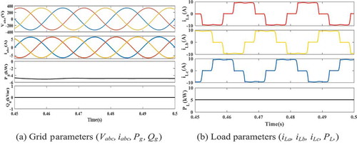
4.1. Case-1: performance analysis of GIPVS using linear and nonlinear load

Figure 8. Performance analysis of the GIPVS under-balanced linear load.

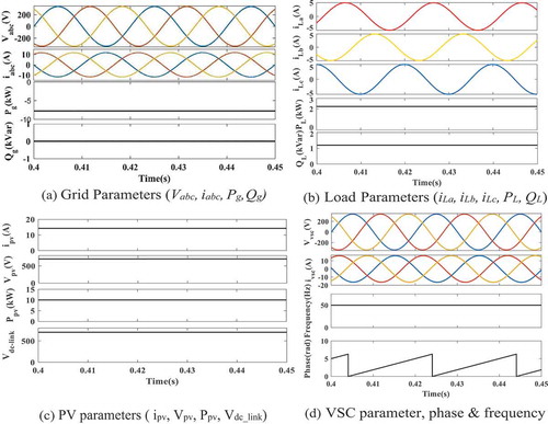
The steady-state performance analysis of the grid integrated PV system is shown in Figure 8. In this case, a linear load of 2.25 kW and nonlinear load of 5.235 kW is considered for performance analysis. The performances of grid potential (V_abc), grid current (i_abc), current and voltage across the VSC (i_vsc and V_vsc), load currents (i_La, i_Lb, i_Lc), power extracted from PV array (P_pv), behaviour of PV array through its terminal voltage (V_pv), and the terminal current (I_pv), voltage across the DC-link capacitor (V_dc-link), real and reactive power transmitted to the grid as well as to the load are shown. Since the reactive power at the grid is equivalent to zero, so it shows that the power factor approaches to unity. DC-link voltage is also maintained constant at its desired value of 700 V through the ICIR MPPT mechanism as shown in Figure 8. The power transmission between the PV source and utility grid is also shown in Figure 8. The negative grid active power indicates the flow of real power from PV source to integrated grid whereas the positive active power indicates the consumption of power by the load. It is observed from the figure that approximately 2.25 kW is consumed by the load and the remaining 7.75 kW is fed to the grid which is negative in nature as shown in Figure 8a.

When the nonlinear load of six-pulse diode bridge rectifier connected with the series RL load having R = 60Ω and L = 100mH is used, the value of the parameters is changed due to the load characteristics. The load voltage is calculated as $V_0=3\times \sqrt{2}\times 415/\pi =560.4V$ and the power consumed by the load is $P_L={560.4}^2/60=5.235kW$. Thus, the remaining $P_{pv}\left(10\right)-P_L\left(5.23\right)\approx P_g\left(4.8kW\right)$power is fed to the grid as shown in Figure 9a. Negative power indicates power flow in reverse direction, i.e. PV source to the grid.

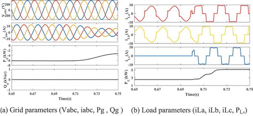
Figure 9. Performance analysis of the GIPVS under nonlinear load.

Similarly, in case of unbalancing when the c-phase is disconnected from 0.6 s to 0.7 s as shown in Figure 10, the power consumed by the load is decreased from 5.23 kW to 2.3 kW during this period. Thus, the power fed to the grid increases to approximately 7 kW excluding losses as shown in Figure 10a.

Figure 10. Transient performances of the GIPV system under-unbalanced nonlinear load.

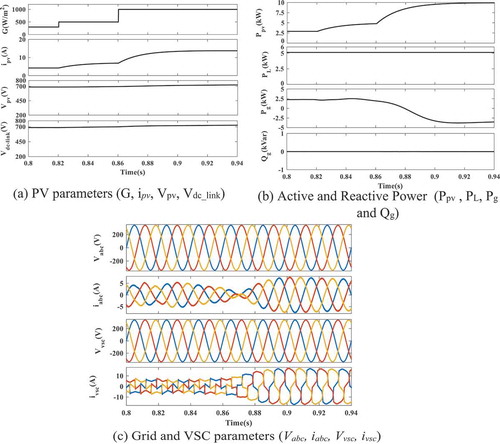
4.2. Case-2: performance analysis under variation of solar insolation

From the mathematical analysis of PV Cell modelling, it is observed that when the solar irradiance G changes the current through the PV array (i_pv) changes proportionately thus the power flow from PV array (P_pv) also changes following the change in G. In case-2, G varies from 0 to 1000W/m² in three stages. Initially, G kept at 300 W/m² at 0.8 s at that time i_pv is approximately 4 A and the corresponding power P_pv is about 2.9 kW, which is not sufficient to deliver power to a load of 5.235 kW. Hence, the grid is supplying the shortage power of 2.3 kW to the load, which is positive in nature as shown in Figure 11b. In the second stage of operation again G increases from 300W/m² to 500W/m² at 0.82 s, the nature of the characteristics is same as aforesaid, but the value of the parameters is changed according to increase in G. When in third stage G is increased from 500W/m² to 1000W/m² at 0.86 s the power flows from PV source to the grid because of G of 1000W/m² the rated P_pv of 10kW is attained and it is sufficient to drive the existing load of 5.235 kW. With the change in G, theV_dc-link remain constant at 700 V and the power factor is maintained at unity. The characteristics of Grid and VSC are also shown in Figure 11c.

Figure 11. Performance of GIPVS under variation of solar irradiance.

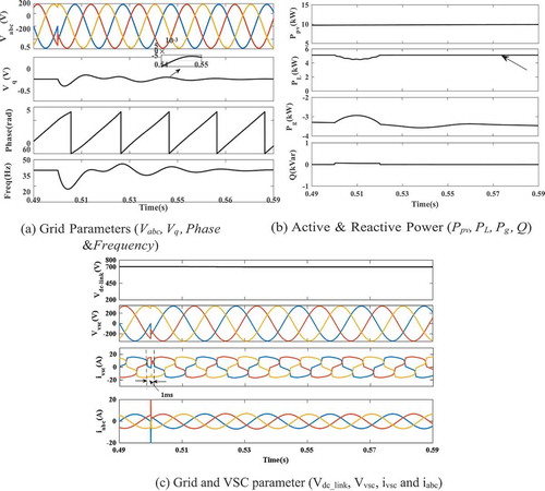
4.3. Case-3: analysis of GIPVS with phase angle jump of −40°

In the above four cases, the performance of the proposed DCFAIA algorithm is tested by changing load and irradiance. It is seen that the exchange of power flow between the grid and the PV source is accomplished effectively. In the following cases, the performance of DCFAIA is analysed under different grid abnormalities. In this case, the phase angle of the grid voltages undergoes a phase angle hop of – 40^◦ to test the behaviour of DCFAIA. The simulation results are shown in Figure 12. In Figure 12a, it is seen that at 0.5 s the phase angle changed by – 40^◦, which corresponds to a phase error of ∆θ = 0.698rad. From the phase error ∆θ, V_q = sin ∆θ ≈ ∆θ = 0.698. It is considered that when $V_q<1\mathrm{\%}\Rightarrow 0.698\times 0.01\simeq 0.007$, then the transient error tends to zero. With the aforesaid criteria of transient analysis, it is noticed from Figure 12a in the zoomed portion of V_q that the phase error takes approximately 50 ms to reach less than 1% of its calculated value. It is also seen that the VSC parameters change suddenly and settle to its original value within 1 ms as shown in Figure 12c. Similarly, the change in phase jump unbalances the reactive power suddenly and with the effectiveness of DCFAIA, it reaches to the zero value within 10 ms and ensures UPF operation as shown in Figure 12b.

Figure 12. Performance of GIPVS with phase angle jump of – 40◦.

4.4. Case-4: analysis of GIPVS with a step-change in the frequency of +3 Hz

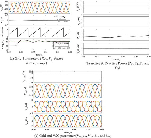
Figure 13 shows the performance of GIPVS when the grid voltage experiences a frequency change of +3Hz at 0.5 s. It is generally happening in the integrated system because of high active loading. The performance shown in Figure 13a depicts the effectiveness of DSCPLL when the fundamental frequency of 50 Hz increases to 53 Hz. Effectiveness of the DSCPLL is judged from transient parameters, i.e. the percentage of overshoot and the settling time. It is noticed from the zoomed portion of the frequency curve that the estimated frequency settles to its new value within a tolerance of ±2% of 53 Hz, i.e. 53*0.98 = 51.94 Hz within 30 ms and the percentage of overshot is found to be 33.33% of the total change. It is also seen that with the step-change in frequency; phase error of 1.432° is introduced in 0.5 s to the system which does not affect the overall system adversely. The active, reactive power flow and the other grid and VSC parameters during the step change of frequency are also shown in Figure 13, where major variations are not observed.

Figure 13. Performance of GIPVS with step change in frequency of +3 Hz.

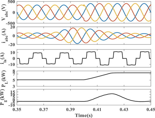
4.5. Case-5: performance analysis of GIPVS under change in amplitude of grid voltage by ±20%

The performance of the GIPVS is analysed by varying the amplitude of the grid voltage by 20%. This type of cases is commonly interpreted as sag or swell conditions. In the case of sag, the voltage decreases whereas the voltage rises suddenly in case of swell. These cases are very common in grid-integrated system. To analyse the performance of the GIPVS under sag and swell conditions, the grid voltage is changed during the period 0.35 s to 0.45 s as shown in Figures 14 and 15. In case of sag, when the grid voltage decreases, the grid current rises but the power consumed by the load decreases due to decrease in load voltage and at the same time, the power fed to the grid increases as shown in Figure 14. Whereas the reverse activities are noticed in Figure 15 in case of swell.

Figure 14. Performance of GIPVS under voltage sag.

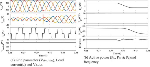
Figure 15. Performance of GIPVS under-voltage swell.

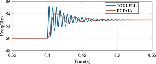
4.6. Case-6: comparative analysis of TOGI-FLL and DCFAIA

Comparative analysis between Third-order generalised integrator-based FLL (TOGI-FLL) and the proposed DCFAIA is made via frequency tracking capability when the grid voltage undergoes a step change of +3 Hz at 0.4 s. It is found from Figure 16 that in TOGI-FLL settling time and peak overshoot is more than that of proposed DCFAIA. Since the peak overshot is less in DCFAIA the effect of phase error is also less as discussed in case-3.

Figure 16. Frequency tracking capability between TOGI-FLL and DCFAIA.

4.7. Case-7: comparative analysis of DCFAIA with conventional methods

To judge the performance of the proposed DCFAIA, the estimation of active weight component of different control schemes is compared with DCFAIA. Since in adverse and steady condition, the active weight is responsible for estimating the reference grid current which enables the VSC to work on different conditions; hence, it can give better comparative analysis. To do so an intentional disturbance in c-phase has been made in simulation during the period 0.4–0.6 s as shown in Figure 17.

Figure 17. Comparative response of average active weight component/average load current (i_lavg) between LMF, DNLMS, DCFAIA, and SRFPLL Algorithm.

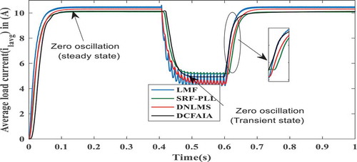
It is noticed from Figure 17 that the peak oscillation during steady and dynamic conditions is almost zero in DCFAIA as compared to conventional methods like LMF, DNLMS, and SRFPLL. It is also noticed that the convergence rate is faster in DCFAIA where no suitable step sizes are required unlike LMS algorithms. The comparative analysis is given in Table 1.

Table 1. Comparative result analysis of LMF, DNLMS, SRF-PLL and DCFAIA.

	Steady State		Dynamic State
Control Algorithms	Precision	Oscillation	Amplitude of Oscillation	Convergence rate
LMF	Poor	High	More	Faster
DNLMS	Good	Less	Less	Slower
DCFAIA	Better	Zero	Zero	Faster
SRFPLL	Good	Zero	Less	Slower

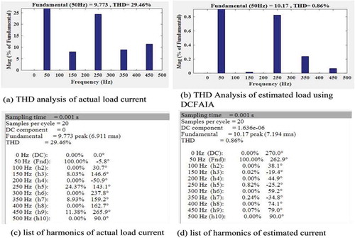
4.8. Case-8: THD analysis

It has claimed in the objective that DC offset will be zero and some of the selective harmonics will be attenuated by DCFAIA. The THD analysis shown in Figure 18 depicts the verification of the statement claimed in section 3 about selective harmonic elimination/attenuation. From Figure 18c, it is observed that before estimation, the percentage of harmonic distortion due to 3^rd(zero sequence harmonics), 5^th(-ve sequence harmonic), 7^th (+ve sequence harmonic) and 9^th (zero-sequence harmonic) order harmonics are found to be 8.03%, 24.37%, 8.93%, and 11.38%, respectively, but after estimation using DCFAIA the % of THD due to 3^rd,5^th, 7^thand 9^th order harmonics are reduced to 0.02%, 0.82%, 0.24%, and 0.07%, respectively, as shown in Figure 18d. It shows that the fundamental extraction of load current is effective and can adapt to any adversities. Figure 18(c,d), shows the order of harmonics presents in the load current. Each order of the harmonics is represented by an amplitude and a phase angle, where the amplitude is measured with respect to the peak value of the fundamental current in percentage, and the corresponding angle represents the position with respect to the time at which, the THD is evaluated.

Figure 18. Harmonic Analysis of Performance Parameters.

Experimental validation of DCFAIA control scheme

A prototype model of GIPVS as shown in Figure 19 has been experimented for validation of the proposed algorithm. In the experimental set up a single-phase prototype model is developed to test the effectiveness of the proposed algorithm. In this setup, the algorithm is modelled using LabVIEW software and for the interfacing of signal between real-time hardware setup and the computer a Data Acquisition (DAQ) device USB6008 is used. The detail hardware setup is shown in Figure 20. The input signals are measured using voltage sensors (VOLTSENS) and current sensors (ACS712). The load current (i_l), current through the PV module (i_pv), the grid voltage (v_g) and voltage across PV module (v_pv) are sensed using assigned voltage and current sensors and then connected to the analog input channels (AI) 0–3 (pin out[2,5,8,11], respectively) of the DAQ card. As the operating limit of the DAQ-AI ports is limited to 5 V, the input analog signals are accordingly calibrated using voltage and current sensors with the help of step-down transformer, current transformer, and necessary circuitry. Then, the signals acquired through sensors are conditioned inside the DAQ and then converted to the digital signals via Analog to Digital Converter (ADC) embedded inside the DAQ card and further, the digital signals are processed using LabVIEW software, where the proposed control algorithm is used to generate reference current. However, as the USB6008 is not capable of generating the Pulse width Modulation (PWM) signals, the reference current (i_g*) is generated through the analog output port (AO) (pin out 14).

Figure 19. Prototype model of 1-ph Grid Integrated PV System.

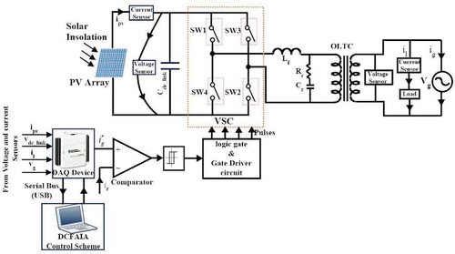
Figure 20. Experimental setup of Grid Integrated PV system.

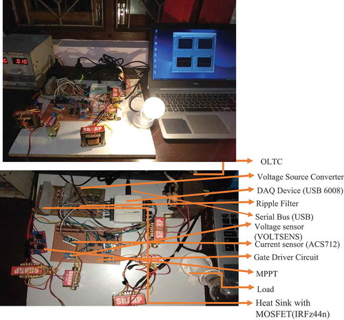
Further, the reference current is compared with the grid current (i_g) using the comparator circuit and PWM signal is generated. The logical conditioning of the single PWM signal is performed to generate four PWM sources for the inverter. The four-legged full-bridge inverter consists of four-power MOSFET (IRFz44n) with diode protection circuits. The output of the inverter is smoothened by LC filter and fed to the load as well as to the grid by using a step-up ON-Load Tap Changer (OLTC) transformer. The results obtained using prototype model are shown in Figure 21.

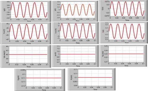
In the performance analysis, the grid voltage (V_g), grid current (i_g), transformer secondary current (i₂), voltage across VSC (V_vsc), current through VSC (i_vsc), load current (i_L), pv current (i_pv), DC-link voltage (V_{dc link}), pv power (P_pv), power consumed by the load(P_L) and power fed to the grid (P_g) are shown in Figure 21.

Figure 21. Performance parameters of prototype model under-balanced load.

Conclusion

DQ-frame Complex Filter-based Adaptive Integral Algorithm is demonstrated with different abnormalities encountered in PV grid integrated system. The benefits of using a pre-filter in PLL are viewed in THD analysis, as it shows the use of SFCF and DSC eliminates the DC offset and selective positive, negative sequence harmonics. Similarly, the transient performance of DCFAIA under a step change in frequency and phase is satisfactory. It is also observed that the unit power factor is maintained and the DC-link voltage remains constant on 700 V under different grid conditions. Comparative analysis between different conventional algorithm invariably says that DCFAIA exhibits better adaptability. The proposed control scheme is validated for a single-phase GIPVS using LabVIEW.

Nomenclature

α0, α1	=	Coefficients of Adaptive Generalised Integrator
∆v	=	Change in voltage
ω	=	Angular frequency
ωlf, ωn, ωe, ∆ω	=	lower cut-off angular frequency, nominal frequency, estimated frequency and frequency error
θ, θe, ∆θ	=	Reference angular position, estimated angular position and position error
ζ, ω0, ωb	=	Damping factor, damping frequency, bandwidth
fsw	=	Switching frequency
h01	=	overloading factor
ip, ilavg	=	Resultant active weight, Average load current
i*a, i*b, i*c	=	Reference Grid Current
idc_link_loss ipv_ff	=	DC-link loss component, Feed forward component
ilad,ilaq	=	DQ component of a-phase load current
ila,ilb,ilc	=	Load currents of a,b and c phases respectively
ima, imb, imc	=	Fundamental component of load current
Kp,Ki	=	Proportional and integral coefficient of DSCPLL
Kcp,τip	=	Proportional gain and integral time constant of voltage regulator
Lf	=	Inductance value of Interfacing Inductor
mi	=	Modulation Index
Ns,Np	=	Number of PV Modules connected in series and parallel
PL,Pg and Qg	=	Active power flow to the load, active and reactive power flow at the grid
Ppv,Vpv,Ipv	=	Maximum Power, Voltage and Current of PV array
Td,h	=	Delay time, harmonic order
ugpa,ugpb,ugpc	=	In-phase templates
Vq	=	Q-axis rotating frame voltage
Vabc,Iabc	=	Three phase grid voltages and currents
Vdcr, ∆ir	=	Percentage of ripple voltage and ripple current
VLM	=	Peak-to-peak line voltage at the grid
Vpvm, Ipvm	=	Open circuit voltage and Short circuit current of PV module
Vvsc, ivsc, Vt	=	Voltage and current across Voltage Source Converter, Terminal Voltage
V lαβ,V ”αβ	=	Stationary frame voltages before and after DSC Block
G	=	Solar irradiance parameters of the PV System

Disclosure statement

No potential conflict of interest was reported by the authors.

Additional information

Notes on contributors

Satish Choudhury

Satish Choudhury is currently working as an Assistant Professor in the Department of Electrical Engineering, ITER, Siksha ’O’ Anusandhan (Deemed to be University), Bhubaneswar.  His research interests include control of power electronics converter, renewable energy sources, adaptive filtering and grid integration. Email: [email protected].

Bidyadhar Subudhi

Bidyadhar Subudhi is currently working as a Professor in School of Electrical Sciences, Indian Institute of Technology GOA, Goa, India. His research interest include System Identification and Adaptive Control, Control of Photovoltaic system and Microgrid, Active Power Filtering, Wide Area Control of Power System, Control of autonomous underwater vehicles. He is a fellow of the Indian National Academy of Engineering.

Renu Sharma

Renu Sharma is currently working as a Professor in the Department of Electrical Engineering, ITER, Siksha ’O’ Anusandhan (Deemed to be University), Bhubaneswar.  Her research interests include renewable energy sources, energy yielding, optimisation techniques, microgrid, control of power electronics converter, load flow etc.

Appendix I.

The parameters of the PV system are calculated as in Akagi, Watanabe, and Aredes (2017). To obtain 10kW of PV power, N_s number of such modules is connected in series and N_p number of modules is connected in parallel. N_s and N_p are calculated using Equation 30(30) $N_s=\frac{V_{dc\mathrm{\_}link}}{V_{pvm}}=\frac{700}{29.3}=23.89\simeq 24$(30) and Equation 31(31) $N_p=\frac{P_{pv}/V_{dc\mathrm{\_}link}}{I_{pvm}}=\frac{10000/700}{7.47}=1.91\simeq 2$(31) .

(30) $N_s=\frac{V_{dc\mathrm{\_}link}}{V_{pvm}}=\frac{700}{29.3}=23.89\simeq 24$(30)

where V_{dc_link} is the voltage across the DC-link capacitor and V_pvm is the open-circuit voltage of PV module.

(31) $N_p=\frac{P_{pv}/V_{dc\mathrm{\_}link}}{I_{pvm}}=\frac{10000/700}{7.47}=1.91\simeq 2$(31)

where P_pv is the maximum power of PV array and I_pvm is the short circuit current of each module.

(32) $V_{dc\mathrm{\_}link}=\frac{2V_{Lm}}{\sqrt{3}{m}_i}=\frac{2\times \left(\sqrt{2}\times 415\right)}{\sqrt{3}\times 1}\simeq 678V$(32)

where V_LM is the peak-to-peak line voltage at the grid and m_i is the modulation index of Voltage Source Converter. V_{dc link} is chosen as 700 V which is slightly higher than the calculated value 678 V. The capacitance value required to obtain the desired V_{dc link} is calculated as in (Agarwal, Hussain, and Singh 2016).

(33) $C_{dc\mathrm{\_}link}=\frac{P_{pv}/V_{dc\mathrm{\_}link}}{2\omega V_{dcr}}=1624\mu F$(33)

where V_dcr is the percentage of ripple voltage, taken as 2% of V_{dc_link} as per grid codes. ω is the angular frequency in rad/sec. The interfacing inductor to avoid short circuit current as discussed in principle of grid connection is calculated using Equation 34(34) $\begin{array}{c}{L}_f=\frac{\sqrt{3}{m}_i{V}_{dc\mathrm{\_}link}}{12h_{01}{f}_{sw}\mathrm{\Delta }{i}_r}\\ =\frac{\sqrt{3}\times 1\times 700}{12\times 1.2\times 20000\times 0.05\times 14.286}\simeq 5.8mH\end{array}$(34) .

(34) $\begin{array}{c}{L}_f=\frac{\sqrt{3}{m}_i{V}_{dc\mathrm{\_}link}}{12h_{01}{f}_{sw}\mathrm{\Delta }{i}_r}\\ =\frac{\sqrt{3}\times 1\times 700}{12\times 1.2\times 20000\times 0.05\times 14.286}\simeq 5.8mH\end{array}$(34)

where h₀₁ is the overloading factor, f_sw is the switching frequency in Hz and ∆_ir is the percentage of ripple current.

PV-Grid integrated system specifications:

PV voltage (V_pv) = 700 V, rated PV power = 10kW, number of PV modules in series (N_s) = 24, number of PV modules in parallel (N_p) = 2, DC-link capacitor (C_{dc_link}) = 1700µF, Interfacing inductor (L_f) = 6mH, proportional controller gain (K_cp) = 0.4 and integral time constant (τ_ip= 40), line voltage across the grid terminal (V_ab) = 415V (rms).

Hardware Specifications: V_pv= 42 V, i_pv= 7.06 A, V_{dc link}= 40 V, OLTC Transformer ratio = 1:8, primary voltage (rms) = 30 V, secondary voltage (rms) = 230 V, load (incandescent bulb) = 100 W = 0.1 kW, C_{dc_link} = 1000µF, Interfacing inductor (L_f)= 3mH.

Appendix–II

List of abbreviations

DCFAIA	=	DQ-frame Complex Filter-based Adaptive Integral Algorithm
DSCPLL	=	Delayed Signal Cancellation Phase-Locked Loop
VSSLMS	=	Variable Step Size Least Mean Square
SRFPLL	=	Synchronous Reference Frame Phase-Locked Loop
DNLMS	=	De-correlation Normalised Least Mean Square
GIPVS	=	Grid Integrated Photovoltaic System
ISOGI	=	Improved Second-Order Generalised Integrator
MPPT	=	Maximum Power Point Tracking
SOGI	=	Second-Order Generalised Integrator
TOGI	=	Third Order Generalised Integrator
ICIR	=	Incremental Conductance with Integral Regulator
CLTF	=	Closed Loop Transfer Function
SFCF	=	Stationary Frame Complex Filter
LMF	=	Least Mean Fourth
PLL	=	Phase-Locked Loop
FLL	=	Frequency Locked Loop
MSD	=	Mean Square Deviation
ICIR	=	Incremental Conductance with Integral Regulator
AGI	=	Adaptive Generalised Integrator
BPF	=	Band Pass Filter
ZCD	=	Zero Cross Detector
VSC	=	Voltage Source Converter
P&O	=	Perturb & Observe
S&H	=	Sample & Hold
PV	=	Photovoltaic
IC	=	Incremental Conductance

References

- Agarwal, R. K., I. Hussain, and B. Singh. 2016. “Lmf-based Control Algorithm for Single Stage Three-phase Grid Integrated Solar Pv System.” IEEE Transactions on Sustainable Energy 7 (4): 1379–1387. doi:10.1109/TSTE.2016.2553181.
- Akagi, H., E. H. Watanabe, and M. Aredes. 2017. “Instantaneous Power Theory and Applications to Power Conditioning.” In John Wiley & Sons 62, edited by M. E. El-Hawary. Hoboken, NJ: John Wiley & Sons.
- Beniwal, N., I. Hussain, and B. Singh. 2017. “Hybrid Vss–LMS–lmf Based Adap- Tive Control of Spv-dstatcom System under Distorted Grid Conditions.” IET Renewable Power Generation 12 (3): 311–322. doi:10.1049/iet-rpg.2016.0868.
- Blaabjerg, F., R. Teodorescu, M. Liserre, and A. V. Timbus. 2006. “Overview of Control and Grid Synchronization for Distributed Power Generation Systems.” IEEE Transactions on Industrial Electronics 53 (5): 1398–1409. doi:10.1109/TIE.2006.881997.
- Bridge, G., S. Barr, S. Bouzarovski, M. Bradshaw, E. Brown, H. Bulkeley, and G. Walker. 2018. Energy and Society: A Critical Perspective (pp.1–12). London: Routledge. doi: 10.4324/9781351019026
- Choudhury, S., B. Dash, and R. Sharma. 2019. “Rejection of Effect of Non- Linearities in a Pv Grid Integrated System Using Vss-sdlms Scheme.” International Journal of Engineering and Advanced Technology 9 (1): 4549–4555.
- Freijedo, F. D., A. G. Yepes, O. Lopez, A. Vidal, and J. Doval-Gandoy. 2011. “Three- Phase Plls with Fast Postfault Retracking and Steady-state Rejection of Voltage Unbalance and Harmonics by Means of Lead Compensation.” IEEE Transactions on Power Electronics 26 (1): 85–97. doi:10.1109/TPEL.2010.2051818.
- Golestan, S., M. Ramezani, J. M. Guerrero, and M. Monfared. 2015. “Dq-frame Cascaded Delayed Signal Cancellation-based Pll: Analysis, Design, and Comparison with Moving Average Filter-based Pll.” IEEE Transactions on Power Electronics 30 (3): 1618–1632. doi:10.1109/TPEL.2014.2315872.
- Li, W., X. Ruan, C. Bao, D. Pan, and X. Wang. 2014. “Grid Synchronization Systems of Three-phase Grid-connected Power Converters: A Complex-vector- Filter Perspective.” IEEE Transactions on Industrial Electronics 61 (4): 1855–1870. doi:10.1109/TIE.2013.2262762.
- Libo, W., Z. Zhengming, and L. Jianzheng. 2007. “A Single-stage Three-phase Grid- Connected Photovoltaic System with Modified Mppt Method and Reactive Power Compensation.” IEEE Transactions on Energy Conversion 22 (4): 881–886. doi:10.1109/TEC.2007.895461.
- Mojiri, M., M. Karimi-Ghartemani, and A. Bakhshai. 2007. “Estimation of Power System Frequency Using an Adaptive Notch Filter.” IEEE Transactions on Instrumentation and Measurement 56 (6): 2470–2477. doi:10.1109/TIM.2007.908631.
- Pradhan, S., I. Hussain, B. Singh, and B. K. Panigrahi. 2018. “Performance Improvement of Grid Integrated Solar Pv System Using Dnlms Control Algo- Rithm.” IEEE Transactions on Industry Applications. 55(1): 78–91. doi: 10.1109/TIA.2018.2863652
- Rout, A., S. Samantara, G. Dash, S. Choudhury, R. Sharma, and B. Dash (2014). “Modelling and Simulation of Hybrid Mppt Based Standalone Pv System with Upgraded Multilevel Inverter”. In 2014 Annual IEEE India Conference (INDICON) (pp. 1-6). IEEE, Pune, India. doi: 10.1109/INDICON.2014.7030423
- Salas, V., E. Olias, A. Barrado, and A. Lazaro. 2006. “Review of the Maximum Power Point Tracking Algorithms for Stand-alone Photovoltaic Systems.” Solar Energy Materials and Solar Cells 90 (11): 1555–1578. doi:10.1016/j.solmat.2005.10.023.
- Shah, P., I. Hussain, and B. Singh. 2019. “Single-stage Secs Interfaced with Grid Using Isogi-fll-based Control Algorithm.” IEEE Transactions on Industry Applications 55 (1): 701–711. doi:10.1109/TIA.2018.2869880.
- Singh, B., C. Jain, and S. Goel. 2014. “Ilst Control Algorithm of Single-stage Dual Purpose Grid Connected Solar Pv System.” IEEE Transactions on Power Electronics 29 (10): 5347–5357. doi:10.1109/TPEL.2013.2293656.
- Subudhi, B., and R. Pradhan. 2013. “A Comparative Study on Maximum Power Point Tracking Techniques for Photovoltaic Power Systems.” IEEE Transactions on Sustainable Energy 4 (1): 89–98. doi:10.1109/TSTE.2012.2202294.
- Swain, S., and B. Subudhi. 2017. “A New Grid Synchronisation Scheme for A Three-phase Pv System Using Self-tuning Filtering Approach.” IET Generation, Transmission & Distribution 11 (14): 3557–3567. doi:10.1049/iet-gtd.2017.0142.
- Vedantham, S., S. Kumar, B. Singh, and S. Mishra. 2017. “Fuzzy Logic Gain- Tuned Adaptive Second-order Gi-based Multi-objective Control for Reliable Operation of Grid-interfaced Photovoltaic System.” IET Generation, Transmission & Distribution 12 (5): 1153–1163. doi:10.1049/iet-gtd.2017.0958.
- Walach, E., and B. Widrow. 1984. “The Least Mean Fourth (Lmf) Adaptive Algorithm and Its Family.” IEEE Transactions on Information Theory 30 (2): 275–283. doi:10.1109/TIT.1984.1056886.
- Wang, Y. F., and Y. W. Li. 2011. “Grid Synchronization Pll Based on Cascaded Delayed Signal Cancellation.” IEEE Transactions on Power Electronics 26 (7): 1987–1997. doi:10.1109/TPEL.2010.2099669.