A sustainable approach to improve the efficiency of earth pipe cooling system

ABSTRACT

Earth pipe cooling (EPC) is a type of passive cooling system that takes advantage of the nearly constant underground temperature of the Earth to cool the atmospheric air in a confined space. The efficiency of this system depends on several factors, including the size and position of the inlet pipe, the velocity of the incoming air, shape of the cooling spaces and inlet surface pattern. However, ensuring uniform dispersion of the incoming cooled air can also improve the thermal comfort and efficiency of the EPC system, which has been overlooked in most of the existing studies. This paper, in this regard, presents a relevant parametric study to highlight that the efficiency of the EPC can be improved significantly by dispersing the oming flow through the proper utilisation of turbulators near the inlet. Thermal models are developed in ANSYS Fluent to perform this simulation-based study. It is found that the application of turbulators can help to reduce the domain temperature by around 0.8°C, thus saving an additional 0.84 kWh of energy per day for the particular cooling space considered in this study.

KEYWORDS:

• Earth pipe cooling
• passive cooling
• sustainable energy
• turbulators

1. Introduction

Air conditioning by vapour compression and vapour absorption is widely used all over the world for industrial and residential thermal comfort (Wang 2000). However, this extensively used vapour compression system requires high-grade energy consumption, and with the rapid growth of the population, the demand for energy is also increasing drastically. Besides, the depletion of the ozone layer by chlorofluorocarbons (CFCs), which is highly related to the air conditioning systems is accelerating global warming and thereby posing threats to humankind’s existence (Bolaji and Huan 2013). Significant efforts are now being placed all over the world to develop efficient, environmentally friendly and cost-effective air conditioning and refrigeration system. Zero energy building is such a concept attaining success all over the world for sustainable energy management of a building these days (Torcellini et al. 2006).

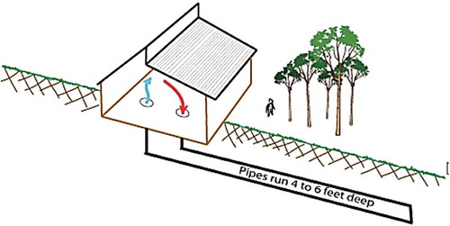
Passive cooling is a state-of-the-art technique of zero energy building design (Cao, Dai, and Liu 2016), and EPC is one of the most prominent passive cooling techniques which uses the Earth soil as a heat sink to dump the excess heat from atmospheric air. In this method, hot outdoor air will pass through pipes buried at a certain depth beneath the ground. This pipe acts as a heat exchanger between the air inside the pipe and the Earth-soil. The hot air enters the pipe beneath the Earth and releases the heat to the cooler soil. The length and layout of the piping system ensure proper heat transfer. The comparatively colder air returns to the closed space above the Earth’s surface to complete the cycle. The sketch of a simplified EPC system is shown in Figure 1. If air is not cooled enough, the temperature can be further reduced using the interconnected air-conditioning system.

Figure 1. Simplified sketch of a passive earth pipe cooling (EPC) system (Source: http://www.resilience.org).

Several studies, including both experimental and simulation, have been performed to fetch the effectiveness, feasibility and efficiency of the EPC system. As the Earth’s surface plays the most vital role in this EPC system, the impact of the Earth’s soil on the cooling performance is studied by Mihalakakou et al. (1997). This study predicts the daily and annual variation of ground surface temperature based on the transient heat conduction differential equation. A parametrical model is also developed by Mihalakakou et al. (1995) to study the effect of pipe length, radius, and air velocity on the system’s performance. An implicit and transient model is developed by Wu, Wang, and Zhu (2007) using Computational Fluid Dynamics (CFD) based PHOENICS software to study the effects of input parameters (i.e. air flow rate, depth, pipe dimensions) on the performance of EPC system. It has been suggested from a recent case study that the room temperature can be reduced up to 1.05 ° C and 1.82 ° C, with horizontal earth pipe cooling system (HEPC) and vertical earth pipe cooling system (VEPC) respectively (Ahmed et al. 2015). The cost-effectiveness of this environment-friendly system can clearly be identified from annual load savings. The maximum annual savings from these HEPC and VEPC systems were found to be 7.93% and 8.82% of the total cost, where the total cost is 2042 and 2743 AUD, respectively.

The heat exchange behaviour between the atmosphere and the ground also impacts the design of EPC system. Recently, Lin et al. (2018) studied one such problem and investigated the cooling performance of two-phase closed thermosyphon. There are also several practical case-based studies regarding EPC systems that can be found in the literature. The cooling capacity of the earth pipe heat exchanger in desert climates is studied by Ajmi, Loveday, and Hanby (2006). The outlet air temperature and cooling potential had been predicted using TRNSYS-IISIBAT environment for the hot, arid climate. This simulation study shows a decrease of 30% energy in the summer season using the EPC system. Greenhouse associated with the EPC system is developed and studied by Ghosal et al. (2005) to understand the significance of earth pipe cooling. Ground air collector and earth air heat exchanger were used here to experimentally study the potential of using the stored thermal energy of the ground. It had been found that air temperature is 2–3°C higher in ground air collectors than in the earth air heat exchanger. Sodha et al. (1985) studied the effectiveness of the EPC system for a hospital building complex in India. Though the heating capacity is not enough for the hospital building complex, the system shows a heating capacity of 269 KWh and a cooling capacity of approximately 512 KWh for an 80 m long tunnel.

As can be seen, EPC attracted noteworthy attention as a low energy passive cooling technique, and a significant number of studies are performed to improve its efficiency considering various factors, as described above. However, the efficiency of an earth pipe cooling system also depends on the proper circulation of incoming air inside the cooling space, which is not addressed adequately in the existing literature. In this study, therefore, the emphasis is provided on maximising the system performance by engineering the inlet pipe’s design to ensure better circulation of the incoming cooled air. It is well known that aerofoil can affect a flow circulation significantly, and the angle of attack & shapes of aerofoil play an important role in determining the flow pattern. For a small angle of attack, inviscid flow shows minor modifications. However, flow separation dominates as the angle of attack increases, and eventually, a strong viscid-inviscid interaction may occur (Rhie and Chow 1983).

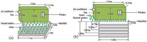
Keeping this in mind, a new approach is adopted in this study by adding aerofoil shaped turbulators in the inlet of the cooling domain to improve the dispersion of the incoming cooled air. Parameters like surface contact ratio have been studied to understand its effect on incoming airflow. A theoretical simulation model is developed to study the operational efficiency of this passive EPC system. This model is designed based on the earth pipe experimental system used by Ahmed et al. (2015) at Central Queensland University, Rockhampton, Australia. The experimental model used by them has two shipping containers, each with a dimension of 5.63 m x 2.14 m x 2.26 m. A series of buried pipes are used to pass air into the room using a fan installed inside the pipe to suck intake air. Both horizontal and vertical alignment of buried pipes had been used to study the EPC system. The earth pipe system has been installed along with air conditioners in this experimental study (Figure 2). The main objective of this setup is to run the air conditioners using lower energy with the help of the passive cooling system. To reduce the amount of solar energy absorbed by the soil surface, trees were planted to shade the soil above the cooling pipes.

Figure 2. Diagram for earth pipe cooling system (Ahmed et al. 2015): (a) Horizontal (b) Vertical.

The numerical model developed in this study is first validated with this experimental analysis. After that, a comprehensive parametric study is performed to understand the effectiveness and efficiency of the aerofoil shaped turbulators towards the improvement of the EPC system. Besides, this study aims to provide a simulation model of the EPC system, which can be further improved in the future by adding more design features.

2. Numerical modelling and validation

2.1. Numerical setup

Earth Pipe cooling (EPC) is a heat transfer process. Computational fluid dynamics (CFD) is a powerful and convenient method used for heat transfer studies over many years. A CFD based solver ‘ANSYS 16.2 Fluent solver’ is used for this study, which is based on the finite volume method. There are several models that can be used to satisfy the physics of the turbulent flow. However, in order to keep consistent with the EPC system of Ahmed et al. (2015), the k – ε turbulence model has been used to simulate the EPC system developed in this study. This model has been extensively used in heat transfer and industrial flow simulations because of its reliability. The boundary conditions are also kept the same as of Ahmed et al. (2015), which are shown in Table 1. An efficient Density-based solver approach is set for the numerical solution. The solution is steady-state and PRESTO scheme is used for pressure term discretisation, momentum, turbulent kinetic energy and turbulent dissipation rate. To ensure the highest accuracy, the first-order upwind scheme is used in the simulation. All residuals are taken to 1e⁻⁰⁶ for better convergence, and to ensure the stability the second-order implicit discretisation scheme has been used.

Table 1. Boundary conditions for both the experimental and simulation model (Ahmed et al. 2015).

Parameters	Value
Inlet velocity	1.1 m/s
Inlet Temperature	20.05°C
Room Temperature	24.90°C
Air Thermal Conductivity	0.024 W/(m.K)
Air Density	1.204 kg/m^2
Specific Heat of air	1006.43 J/kg.k
Air viscosity	1.850387e-05 kg/m.s
Initial system pressure	101.325 KPa

2.2. Model description

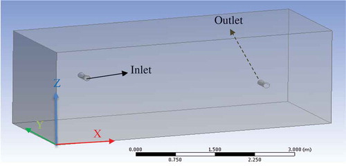
In order to be compatible with the experimental system of HEPC, a domain of 5.63 × 2.14x2.26 m dimension having an inlet diameter of 0.125 m is constructed (as shown in Figure 3) with the help of CATIA. This system is similar to the EPC experimental system designed by Ahmed et al. (2015). An outlet has also been included on the opposite side of the inlet in order to keep the system more compatible with the experimental system of HEPC. The diameter of the outlet is kept the same as the inlet diameter, and the positions of the outlet and inlet with respect to the coordinate origin are (5.18, 2.14, 0.375) and (0.731, 0.0, 4.561) respectively. A grid sensitivity study is performed for this simulation model of the present study, followed by validation with the experimental study mentioned above. Later the model will be modified by moving the inlet towards the middle of the xz surface and adding different numbers of aerofoil shape turbulators around the inlet.

Figure 3. Simulation domain with the coordinate system.

2.3. Grid sensitivity study

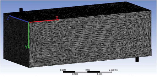
The simulations for sensitivity study are performed successively on Hex dominant meshing and have been done with refinement near the outlet and inlet as demonstrated in Figure 4. Four different meshes are used to perform the mesh independency study as shown in Table 2. A single value of inlet air velocity (m/s) is used for this mesh independency study and the entire simulation domain is divided into eight equal segments. The air velocity right in the middle of all these segments is then compared for these four mesh scenarios. As can be seen in Table 2, both the 283 K and 380 K node cases exhibit similar air velocity across all the segments. Therefore, 283 K nodes are used in the rest of the simulations.

Table 2. Comparison of air velocity (m/s) at different locations of the cooling space.

	Coordinates of the midpoints of eight segments of the entire domain (m)
Number of Nodes	X = 1.075 Y = 0.532 Z = 0.565	X = 1.075 Y = 0.532 Z = 1.695	X = 4.225 Y = 0.532 Z = 0.565	X = 4.225 Y = 1.597 Z = 1.695	X = 1.407 Y = 1.597 Z = 0.565	X = 1.407 Y = 1.597 Z = 1.695	X = 4.225 Y = 1.597 Z = 0.565	X = 4.225 Y = 1.597 Z = 1.695
70 K	0.03933	0.035174	0.016456	0.024685	0.035669	0.03274	0.013928	0.024685
145 K	0.00176	0.004373	0.003774	0.001917	0.003207	0.00419	0.003387	0.001917
283 K	0.00169	0.004460	0.003821	0.002139	0.003168	0.00400	0.003420	0.002139
380 K	0.00168	0.004458	0.003819	0.002154	0.003147	0.00398	0.003403	0.002154

Figure 4. Meshed domain of the simulation model (280 K nodes).

2.4. Validation of the numerical model

As stated in section 2.2, the numerical model developed for the current simulation study is compared with the experimental analysis conducted by Ahmed et al. (2015). In one of their experimental studies, setup consists of horizontal buried pipes connected to a shipping container (the cooling space) is used, and it was installed at Central Queensland University, Australia. In this Horizontal Earth Pipe Cooling (HEPC) system, the container was fitted with two PVC pipes of outside diameter 0.125 m, which works as the manifolds. Intake air comes through one of these manifolds and passes through a series of 20 corrugated buried pipes aligned horizontally and moves into the room through another manifold (marked as ‘inlet’ in Figure 3).

The focus of the current numerical study, however, is to improve the circulation of cooled air inside the cooling space. Therefore, in this numerical model, outside piping and associated setup are ignored, and it is assumed that the incoming air has a fixed average temperature and velocity. Besides, an average fixed temperature is considered for the walls of the cooling space, though, in experimental analysis the wall temperature was varying as it was exposed to the dynamic outside weather. However, to keep the system consistent with the experimental model, the dimension of the room has been kept the same at 5.63 × 2.14x2.26 m and all other relevant setup parameters are also kept the same as that of experimental study (Table 1).

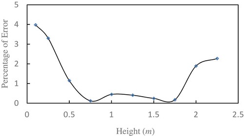
Simulation is then performed, and temperatures at the centre of the cooling space are measured along the height of the container, at an interval of 0.25 m. Table 3 shows the comparison of the results obtained from the simulation with the corresponding experimental values. As can be seen, the numerical values match quite well with the experimental results except near the bottom and top of the cooling spaces. The percentage of errors plotted in Figure 5 shows that the errors are nearly 1 percent in locations (points) that are away from the boundaries. The reason behind higher errors closer to the boundaries might be due to the fact that unlike the experiment, a constant wall temperature was considered in this simulation.

Table 3. Temperatures along the centre line of the cooling space (experimental vs numerical values).

Height (m)	Experimental Temp (^oC)	Numerical Temp (^oC)
0.25	25.490	24.650
0.50	24.930	24.640
0.75	24.670	24.640
1.00	24.510	24.639
1.25	24.840	24.739
1.50	24.580	24.641
1.75	24.600	24.643
2.00	24.190	24.647

Figure 5. Percentage of error in room temperature measured by numerical analysis.

2.5. Cooling load calculation

A cooling load calculation is presented in this section, which will be used later to measure the efficiency of the developed numerical model. The experimental setup of Ahmed et al. (2015) is used to perform this cooling load calculation.

The total cooling load of a building consists of heat transferred through the building envelope, i.e. walls, roof, floor, windows, doors etc. and heat generated by the occupants, equipment, and lights. The load due to the heat transfer through the envelope is called an external load, while all other loads are called internal loads. The percentage of external versus internal load varies with building type, site climate, and building design. The total cooling load on any building consists of both sensible as well as latent load components. The sensible load affects the dry-bulb temperature, while the latent load affects the moisture content of the conditioned space (Bhatia 2012).

In this present study, the cooling load is calculated for the entire system using CLF/CLTD method. During calculations, the heat gain of the room from several external and internal sources should be taken into account (as depicted in Figure 6). For example, heat gain from conduction through exterior walls, roof, and glass, conduction through interior partitions, ceilings, and floors, solar radiation through glass, heat from lighting, people, equipment and infiltration of outside air through openings.

Figure 6. Room heat gain, Q from various external and internal sources (Pita 2002).

The following mathematical formulations are used for the calculation of cooling load for various sources. Several factors such as building orientation (N, S, E, W, NE, SE, SW, NW), location, external/internal shading, ground reflectance, materials of construction for external walls, roofs, windows, doors, internal walls, partitions, ceiling, insulating materials and thicknesses, external wall and roof colours and amount of glass, type and shading on windows should also be taken into consideration to make the system more compatible with the real scenario (Pita 2002).

2.5.1. For wall: Exposed to sun

(1) $Q_w=A\times U\times CLT{D}_c$(1)

Where,

$Q_w$ = Cooling load for the wall, W

$A$ = Area of the wall, m²

$U$ = Overall heat transfer coefficient for the wall, W.m².${ }^{\circ }C$

$CLT{D}_c$ = Corrected cooling load temperature difference, °C

The cooling load temperature difference (CLTD) is not the actual temperature difference between the outdoor and indoor air. It is a modified value that accounts for the heat storage/time-lag effects.

(2) $CLT{D}_c=\left[CLTD+LM+\left(25.5-T_i\right)+\left(T_a-29.4\right)\right]$(2)

Where,

$CLT{D}_c$ = Cooling load temperature difference, °C

$CLT{D}_c$ = Corrected cooling load temperature difference, °C

$LM$ = Correction for latitude and month

$T_i$ = Inside dry bulb temperature, °C

$T_a$ = Adjacent space temperature, °C

Values of various coefficients in the above equations, such as CLTD, LM, U are taken from the 1997 ASHRAE Fundamentals Handbook (SI) (ASHRAE 1997).

2.5.2. Solar transmission through north glass window

Radiant energy from the sun passes through transparent materials such as glass and becomes a heat gain to the room. The value varies with time, orientation, shading, and storage effect. In the cooling space for this study, a glass window was considered on the north side of the room. The solar cooling load due to that glass window can be found from the following equation:

(3) $Q_{GS}=A_G\times SHGF\times SC\times CLF$(3)

Where,

$Q_{GS}$ = Solar radiation cooling load for glass, W

$A_G$ = Area of glass, m²

$SHGF$= Maximum solar heat gain factor

$SC$= Shading coefficient

$CLF$= Cooling load factor for glass

The maximum solar heat gain factor (SHGF) is the maximum solar heat gain through single clear glass at a given month, orientation, and latitude. The cooling load factor CLF accounts for the storage of part of the solar heat gain. The values of $SHGF,SC$and $CLF$ are also taken from the 1997 ASHRAE Fundamentals Handbook (SI) (ASHRAE 1997).

2.5.3. Heat transfer through the ceiling

(4) $Q=A\times U\times \left(T_a-T_o\right)$(4)

Where,

$Q$ = Heat gain through the ceiling, W

$A$ = Area of the ceiling, m²

$U$ = Overall heat transfer coefficient, W.m².${ }^{\circ }C$

$T_a$ = Adjacent space temperature, °C

$T_o$ = Outside dry bulb temperature, °C

The value of U is taken as 0.18 W.m².${ }^{\circ }C$, following the 2005 ASHRAE Handbook Fundamentals (ASHRAE 2005).

2.5.4. Heat transmission through the floor

(5) $Q=A\times U\times CLTD$(5)

Where,

$Q$ = Heat gain through the floor, W

$A$ = Area of the floor, m²

$U$ = Overall heat transfer coefficient, W.m².${ }^{\circ }C$

$CLTD$ = Cooling load temperature difference, °C

2.5.5. Internal loads

For lighting

(6) $Q=3.4\times W\times BF\times CLF$(6)

$Q$ = Cooling load from lighting, W

$W$ = Lighting capacity, W

$BF$ = Ballast factor

$CLF$ = Cooling load factor for lighting

The factor BF accounts for heat losses in the ballast in fluorescent lamps or other special losses. A typical value of BF is 1.25 for fluorescent lighting. For incandescent lighting, there is no extra loss and BF = 1.0.

The factor CLF accounts for the storage of part of the lighting heat gain. The storage effect depends on how long the lights and cooling system are operating, as well as the building construction, type of lighting fixture, and ventilation rate.

The value of CLF is taken from the 1997 ASHRAE Fundamentals Handbook (SI) (ASHRAE 1997) for 10 hours of operation and 8 hours closed after lights are on.

2.5.6. For people

The heat gain from people is composed of two parts, sensible heat and the latent heat resulting from perspiration. Some of the sensible heat may be absorbed by the heat storage effect, but not the latent heat. The equations for cooling loads from sensible and latent heat gains from people are

(7) $Q_s=q_s\times n\times CLF$(7)

(8) $Q_l=q_l\times n$(8)

Where,

$Q_s$, $Q_l$ = Sensible and latent heat gains (loads), W

$q_s$, $q_l$ = Sensible and latent heat gains per person, W

$n$ = Number of people

$CLF$ = Cooling load factor for people

2.5.7. For infiltration and ventilation

Ventilation air is the amount of outdoor air required to make up for air leaving the space due to equipment exhaust, exfiltration, and as required to maintain indoor air quality for the occupants. Infiltration of air through cracks around windows or doors results in both a sensible and latent heat gain to the rooms.

(9) $Q_{sensible}=1.23\times Q\times \left(T_o-T_i\right)$(9)

(10) $Q_{latent}=3010\times Q\times \left(W_o-W_i\right)$(10)

Where,

$Q_{sensible}$,$Q_{latent}$ = Sensible and latent cooling loads for ventilation and infiltration, W

Q = Ventilation and infiltration rate, L/s

$T_i$ = Inside dry bulb temperature, °C

$T_o$ = Outside dry bulb temperature, °C

$W_i$ = Inside humidity ratio, kg (water)/kg (dry air)

$W_o$ = Outside humidity ratio, kg (water)/kg (dry air)

The overall cooling load is calculated by summing up all the heat gains, i.e. the Q values from Equation (1)(1) $Q_w=A\times U\times CLT{D}_c$(1) to (10). Then considering a 10% safety factor, the total cooling load is obtained from the equation below:

(11) $Q=1.10\times Coolingload$(11)

3. Modification of the inlet design

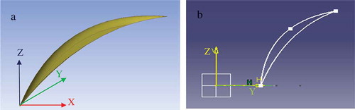
In order to improve the cooling efficiency of the existing HEPC, aerofoil shape turbulators have been introduced around the inlet of the validated simulation model (Figure 7(a)). Both the three and two-dimensional closeup view of the tabulator’s shape is also depicted in Figure 8. Preliminary results obtained from this model are reported in Saha et al. (2018). A total of 12 simulation cases are designed to study the influence of the number of aerofoil shape turbulators and the radius of the circle around which the turbulators are arranged. As shown in Table 4, case 1 is similar to the model studied by Ahmed et al. (2015) in their experimental analysis, except the fact that the inlet is now slightly moved downward to put it in the middle along the z-axis. The coordinate of the inlet for case 1 is (0.731, 0.0, 1.13). For all other cases, N number of aerofoils are added around the perimeter of the circle having radius R. Aerofoil shaped turbulator will spread the air around the inlet and will ensure proper circulation in cooling spaces. The aerofoil arrangement for case 4 (12 aerofoils around a 40 mm radius circle) is shown in Figure 7(b). It should be noted here that except for the number of aerofoils, all other simulation parameters are kept the same in all these 12 cases.

Table 4. Definition of simulation cases.

Case number	N = number of turbulator shaped airfoils	R = radius of the circular pattern (m)
1	0	0
2	6	20
3	9	30
4	12	40
5	15	50
6	18	60
7	4	20
8	2	20
9	8	40
10	4	40
11	10	50
12	5	50

Figure 7. Distribution of aerofoils near the inlet for Case 4: (a) 3D closeup view of the inlet area of the domain, (b) 2 D view of the inlet only.

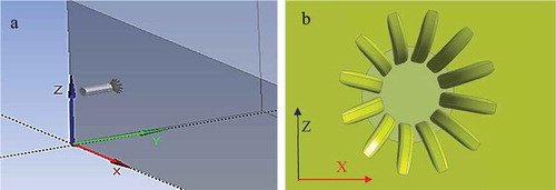
Figure 8. Shape of the single aerofoil shape turbulator: (a) 3 D view, (b) 2 D view.

4. Results and discussion

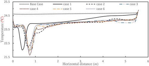
The key variables influencing the performance of the earth pipe cooling system in this paper are the orientation of turbulators, surface contact ratio, the position of the inlet. To demonstrates the effect of all these parameters, the temperatures at various points inside the domain for the first 6 simulation cases are compared along with the validation model (Base Case). Figure 9 shows this comparison – the changes in temperature along the length of the domain by varying the x and keeping y and z fixed at 1.07 m and 1.13 m respectively. As can be seen, the effect of turbulators on reducing temperature is quite noticeable as compared to the base case. The sharp reduction in temperature for all the cases near x = 0.75 m is due to the position of the inlet at that location. It is also observed that the differences in temperature among cases 2 to 6 are not significant. This is because a similar surface contact ratio is used for all these cases, i.e. the number of turbulators is increased proportionately as the radius of the circle increases. Therefore, it can be said that increasing the perimeter of aerofoil’s distribution does not produce a significant impact on temperature reduction. The temperature profile at different height along the vertical centre line of the domain (x = 2.815 m, y = 1.07 m, and z is variable) for these 6 cases are also shown in Table 5. The significant effect of inlet modification on temperature reduction is clearly noticeable from this table as well.

Table 5. Temperatures (⁰ C) at various heights along the centre line of the simulation domain.

Heights (m)	Base Case	Case 1	Case 2	Case 3	Case 4	Case 5	Case 6
0.1	24.658	24.148	23.699	24.090	23.810	23.784	23.842
0.25	24.650	24.273	23.826	23.744	23.931	23.842	23.971
0.5	24.640	24.372	23.944	23.799	24.070	23.921	24.051
0.75	24.640	24.333	23.898	23.852	24.110	23.883	23.982
1	24.639	24.187	23.941	23.967	24.058	23.946	23.965
1.25	24.739	24.190	24.035	24.051	23.994	24.050	24.094
1.5	24.641	24.338	24.096	24.091	23.965	24.108	24.080
1.75	24.643	24.356	24.053	24.108	23.952	24.076	24.050
2	24.647	24.251	23.906	23.944	23.904	23.940	23.952
2.25	24.667	24.419	23.780	24.800	23.731	23.804	23.805
Average (^0 C)	24.650	24.251	23.920	23.910	23.900	23.920	23.979

Figure 9. Temperatures (⁰ C) for various Cases along the horizontal centreline of the domain.

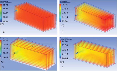
Figure 10 shows the sliced temperature gradients inside the domain for four different cases. As can be seen for the base case (Figure 10(a)), the temperature in the domain is nearly constant everywhere. However, moving the inlet towards the middle position and later adding turbulator shaped aerofoils around the inlet has made significant improvement in temperature reduction, which can be seen in Figure 10(b–d). Besides, as already highlighted in the discussion for Figure 9 and Table 5, the difference in the temperature gradient between case 3 and case 4 is very negligible, and so is for cases 5 and 6 as well.

Figure 10. Sliced temperature gradients: (a) Base Case, (b) Case 1, (c) Case 3, (d) Case 4.

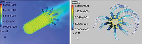
Figure 11 shows the volume rendering of velocity, the circulation of the incoming air inside the three-dimensional simulation domain. As noticed, the circulation is very poor for the base case (Figure 11(a)), whereas it improves as the inlet is moved towards the middle (Figure 11(b)). After that, the inclusion of turbulators significantly spreads the flow velocity inside the domain, thus, improving the cooling efficiency of the incoming air. Figure 12 shows a closer view of the aerofoil effect on the flow velocity and the circulation pattern for case 3. As can be seen, the air starts to diverge as it passes through the inlet and gets adjacent to the aerofoil turbulators (Figure 12(a)). Figure 12(b) shows how the aerofoils affect the streamlines (as seen from inside the domain) and help to spread the airflow to enhance the circulation. The presence of each of the aerofoils creates a wake in the downstream region, and the interactions among all these adjacent wake regions disturb the streamlines, and thereby, ensure an efficient mixing up of the flow.

Figure 11. Volume rendering of temperature contours: (a) Base Case, (b) Case 1, (c) Case 3, (d) Case 4.

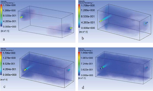
Figure 12. Close up view of flow circulation (Case 3): (a) Velocity gradient, (b) Velocity streamlines.

As already highlighted, the same surface contact ratios for the aerofoils are maintained from case 2 to case 6, resulting in similar improvement on cooling effects for all these cases. From case 7 to case 12, therefore, the surface contact ratio has been varied by changing the number of aerofoils for R = 20, 40 and 50. For example, in case 7 and case 8, the number of aerofoils is reduced in a ratio of 3:2 and 3:1, respectively, as compared to case 2 while keeping the radius constant (R =20). The same procedure is followed for cases 9, 10 and cases 11,12. Figure 13 shows the influence of varying aerofoils number on average temperature changes in the domain. R20 shows the change in temperatures for cases 2,7,8 (with 6, 4 and 2 number of aerofoils respectively while keeping the radius the same at 20 mm). R40 represents cases 4,9,10 and R50 cases 5,11,12. As can be seen, increasing the number of aerofoils while keeping the radius fixed helps to reduce the average domain temperature. However, the reduction rate is higher for a smaller radius compared to the larger periphery. The above discussions clearly highlight the effectiveness of the proposed inlet modification design using aerofoil shaped turbulators

Figure 13. Influence of aerofoil numbers on average domain temperature.

For this present model under study, the cooling load is also calculated considering a room having dimensions identical to the experimental setup of Ahmed et al. (2015), and following the procedures described in section 2.5. The outside walls of the room are considered to be exposed to the sun at a temperature of 35°C and the interior to be maintained at the human comfort temperature 22°C. The total cooling load obtained in this regard is 3200.34 W, i.e. 0.91 TR. Now, the inlet modification proposed in this study shows that interior temperature can be further reduced by around 0.8°C by using this aerofoil shaped turbulators. Thus, while the air conditioning unit of capacity 0.91 TR is required for the normal inlet system, the use of turbulators in the modified inlet design system can reduce the unit capacity requirement for the air conditioning to 0.90 TR, i.e. 3165 W. This represents an energy savings of 35 J per second, translating to power save of 0.84 KWh per day for this particular small room.

5. Conclusion

Earth Pipe Cooling (EPC) is a less expensive passive cooling system that provides maximum thermal comfort of the building occupants without affecting the environment. This system reduces the air conditioning cooling load without emitting greenhouse gas. A simple and cost-effective approach to improve the efficiency of EPC by simply modifying the inlet of the air is presented in this study. A simulation-based parametric study is performed to demonstrate the efficiency of the proposed system. 12 test cases are designed by varying the number of aerofoils and radius of their circular base. It is found that the introduction of aerofoil shape turbulators near the inlet area in circular patterns can further reduce room temperature by around 0.8°C for the particular scenario considered in this study. Such a reduction, in turn, will help to reduce the power consumption by 0.84 KWh per day for this particular small room.

However, more studies, for example, analysing the effect of change of angle of attack of the aerofoil shaped turbulators, varying wall temperatures, changing the initial temperature of the cooling space, experimental analysis to understand the effectiveness of the system can be carried out for a better understanding of this proposed design.

Nomenclature

$A$	=	Area ($m^2$)
$BF$	=	Ballast Factor
$CLF$	=	Cooling Load Factor
$CLTD$	=	Cooling Load Temperature Difference (°C)
$CLT{D}_c$	=	Corrected Cooling Load Temperature Difference (°C)
$LM$	=	Correction for latitude and month
$n$	=	Number of people
$q_s$	=	Sensible heat gain per person (W)
$q_l$	=	Latent heat gain per person (W)
$Q$	=	Heat gain (W)
$SHGF$	=	Solar Heat Gain Factor
$SC$	=	Shading Coefficient
$T_i$	=	Inside dry bulb temperature (°C)
$T_o$	=	Outside dry bulb temperature (°C)
$T_a$	=	Adjacent space temperature (${ }^{\circ }C$)
$TR$	=	Ton of Refrigeration
$U$	=	Overall heat transfer coefficient (W.$m^2{.}^{\circ }C$)
$W$	=	Lighting capacity (W)
$W_o$	=	Outside humidity ratio (kg (water)/kg (dry air))
$W_i$	=	Inside humidity ratio (kg (water)/kg (dry air))

Disclosure statement

No potential conflict of interest was reported by the authors.

Additional information

Notes on contributors

Mahdi-Ul- Ishtiaque

Md. Mahdi-Ul- Ishtiaque is currently working as a lecturer at Sonargaon University, Bangladesh. Before joining here, he completed his BSc in Naval Architecture and Marine Engineering from Bangladesh University of Engineering and Technology in Oct 2018.

Parnab Saha

Parnab Saha is pursuing PhD at Michigan State University under the department of mechanical engineering and working on developing an energy-efficient heat exchanger. He completed his BSc in Naval Architecture and Marine Engineering from BUET (Bangladesh University of Engineering and Technology) in Oct 2017, then joined daffodil international university, Bangladesh as a lecturer and worked there until Dec 2018.

Amit Sutradhar

Amit Sutradhar is a lecturer in the Department of Mechanical Engineering at Dhaka University of Engineering & Technology, Bangladesh. He completed B.Sc. in Mechanical Engineering from Khulna University of Engineering & Technology, Bangladesh, in Mar 2017. Then he joined the Department of Mechanical Engineering at Sonargaon University, Bangladesh as a lecturer and worked there till starting his current position in Jan 2018.

Musanna Galib

Musanna Galib completed B.Sc. (2017) and M.Sc. (2019) in Mechanical Engineering from Bangladesh University of Engineering and Technology (BUET). Then joined Dept. of Mechanical Engineering, BUET as a lecturer and currently working there as an Assistant Professor since Dec 2019.

Mohammed Abdul Hannan

Mohammed Abdul Hannan received a BSc degree (first-class honours) in Naval Architecture and Marine Engineering from Bangladesh University of Engineering and Technology (Mar 2009) and later obtained a Ph.D. from the National University of Singapore in Nov 2014. He was working as a Research Fellow at the National University of Singapore before joining Newcastle University as an Assistant Professor in Aug 2016.

References

- Ahmed, S. F., M. M. K. Khan, M. T. O. Amanullah, M. G. Rasul, and N. M. S. Hassan. 2015. “Performance Assessment of Earth Pipe Cooling System for Low Energy Buildings in a Subtropical Climate.” Energy Conversion and Management 106: 815–825. doi:10.1016/j.enconman.2015.10.030.
- Ajmi, F. A., D. L. Loveday, and V. I. Hanby. 2006. “The Cooling Potential of Earth–air Heat Exchangers for Domestic Buildings in a Desert Climate.” Building and Environment 41: 235–244. doi:10.1016/j.buildenv.2005.01.027.
- ASHRAE. 1997. “Nonresidential Cooling and Heating Load Calculations.” Chap. 28 in 1997 ASHRAE Fundamentals Handbook, 28.39–28.55. Atlanta, GA: SI Edition by the American Society of Heating, Refrigerating and Air-Conditioning Engineers, Inc.
- ASHRAE. 2005. “Residential Cooling and Heating Load Calculations.” Chap. 29 in 2005 ASHRAE Handbook-Fundamentals, 29.14. Atlanta, GA: SI Edition by the American Society of Heating, Refrigerating and Air-Conditioning Engineers, Inc.
- Bhatia, A. 2012. Cooling Load Calculations and Principles., 8. 9 Greyridge Farm Court Stony Point, NY 10980: Continuing Education and Development, Inc. P: (877) 322-5800 F: (877) 322-4774.
- Bolaji, B. O., and Z. Huan. 2013. “Ozone Depletion and Global Warming: Case for the Use of Natural Refrigerant–a Review.” Renewable and Sustainable Energy Reviews 18: 49–54. doi:10.1016/j.rser.2012.10.008.
- Cao, X., X. Dai, and J. Liu. 2016. “Building Energy-consumption Status Worldwide and the State-of-the-art Technologies for Zero-energy Buildings during the past Decade.” Energy and Buildings 128: 198–213. doi:10.1016/j.enbuild.2016.06.089.
- Ghosal, M. K., G. N. Tiwari, D. K. Das, and K. P. Pandey. 2005. “Modeling and Comparative Thermal Performance of Ground Air Collector and Earth Air Heat Exchanger for Heating of Greenhouse.” Energy and Buildings 37 (6): 613–621. doi:10.1016/j.enbuild.2004.09.004.
- Lin, C., Y. Wenbing, L. Yan, and L. Weibo. 2018. “Numerical Simulation on the Performance of Thermosyphon Adopted to Mitigate Thaw Settlement of Embankment in Sandy Permafrost Zone.” Applied Thermal Engineering 128: 1624–1633. doi:10.1016/j.applthermaleng.2017.09.130.
- Mihalakakou, G., M. Santamouris, D. Asimakopoulos, and I. Tselepidaki. 1995. “Parametric Prediction of the Buried Pipes Cooling Potential for Passive Cooling Applications.” Solar Energy 55 (3): 163–173. doi:10.1016/0038-092X(95)00045-S.
- Mihalakakou, G., M. Santamouris, J. O. Lewis, and D. Asimakopoulos. 1997. “On the Application of the Energy Balance Equation to Predict Ground Temperature Profiles.”.” Solar Energy 60 (3–4): 181–190. doi:10.1016/S0038-092X(97)00012-1.
- Pita, E. G. 2002. Air Conditioning Principles and Systems. 4th ed. Upper Saddle River, NJ: Pearson Education, Inc.
- Rhie, C. M., and W. L. Chow. 1983. “Numerical Study of the Turbulent Flow past an Airfoil with Trailing Edge Separation.” AIAA Journal 21 (11): 1525–1532. doi:10.2514/3.8284.
- Saha, P., M. Galib, M. M. U. Ishtiaque, S. R. Akanda, and M. A. Hannan. 2018. “Numerical Study on Improving the Efficiency of the Earth Pipe Cooling System.” International Conference on Civil & Environmental Engineering, ICCEE, Kuala Lumpur, Malaysia 65: 05018. doi:10.1051/e3sconf/20186505018.
- Sodha, M. S., A. K. Sharma, S. P. Singh, N. K. Bansal, and A. Kumar. 1985. “Evaluation of an Earth– Air Tunnel System for Cooling/heating of a Hospital Complex.” Building and Environment 20 (2): 115–122. doi:10.1016/0360-1323(85)90005-8.
- Torcellini, P., S. Pless, M. Deru, and D. Crawley. 2006. Zero Energy Buildings: A Critical Look at the Definition. Golden, CO: National Renewable Energy Lab. (NREL). No. NREL/CP-550-39833.
- Wang, S. K. 2000. Handbook of Air Conditioning and Refrigeration. Vol. 49. New York: McGraw-Hill.
- Wu, H., S. Wang, and D. Zhu. 2007. “Modelling and Evaluation of Cooling Capacity of Earth–air–pipe Systems.” Energy Conversion and Management 48 (5): 1462–1471. doi:10.1016/j.enconman.2006.12.021.