Comparative analysis of single- and multi-criteria container transport modes in Peninsular Malaysia

ABSTRACT

This study investigates the transport of containers via intermodal transport network of Peninsular Malaysia by comparatively analysing the use of trucks, trains and ships with respect to time, CO₂ emission and cost. The study is aimed at proposing the best route/mode of container transport in Peninsular Malaysia. ArcMap and MATLAB were employed to identify the single-objective route/modal choices. The multi-criteria route/modal choices were achieved by integrating the Simple Multi-Attribute Rating Technique (SMART) and sensitivity analysis. The single-objective results indicated that the use of trucks on road was the fastest mode of container transport. However, the combination of ship and train was the most environmental-friendly for Case 1, while transport by ship generated the least CO₂ emission for Case 2. Train was found to be the cheapest mode of container transport, followed by ship and truck. It can be inferred from the multi-criteria analysis that container transport via rail is the ideal and least-cost route and mode of transport.

KEYWORDS:

• Container transport
• single-objective
• multi-criteria
• optimum route
• intermodal network

1. Introduction

In the last six decades, the invention of containerisation has propelled logistics and transportation onto a new stage (Lam and Gu 2016). Standardisation, a key concept of containerisation, facilitates the ease of handling materials along the whole transport chain. This ensures the effective and efficient movement of containers from origin to destination by different transport means (vessel, train, truck) without the need for reorganising/re-handling of the content within (Lee and Song 2017). Studies have revealed the contribution of expansion in global trade and manufacturing industries to the growth in global container shipments. On a global scale, containerised cargoes grew at an annual average rate of 7.6% over the period of 2005 through 2015 (UNESCAP, 2007). The international trade of Malaysia has significantly increased as indicated by an average growth rate of 9.6% during the period 1993––2013 (DSM, 2015). This reflected a remarkable increase in container trade from 900,000 TEUs (the twenty-foot equivalent unit) in 1990 to 20.8 million TEUs in 2013 (Chen, Jeevan, and Cahoon 2016). This is expected to increase further to 36.6 million TEUs by 2020 (Nasir 2014). It was reported that about 45% of the container volumes are local containers entering the Malaysian hinterland (Nasir 2014). However, the associated increase in container movement is encumbered by some challenges such as increase in road congestion, fuel consumption, Greenhouse gas (GHG) production and noise pollution, GHGs, and mainly carbon dioxide (CO₂), methane (CH₄), nitrous oxide (N₂O) and ozone (O₃) are the most studied negative externalities of freight transportation (Demir et al. 2019). CO₂ is the most widespread pollutant that aggravates global warming (Oh and Chua 2010) (Gajanand and Narendran 2013), and is majorly produced by transportation sector (Ong, Mahlia, and Masjuki 2012) (Bergqvist et al. 2015).

Multi-criteria Decision Analysis, usually abbreviated as MCDA, is an analytical tool that evaluates many criteria for making complex decisions with the aim of selecting the best option among alternatives. It is widely being used in different fields of transportation studies such as evaluation of policy measures in passenger transport, strategic decisions, technologies, locations and infrastructure projects (Macharis, De Witte, and Ampe 2009). Basically, making decision using MCDA approaches improves the satisfaction with the decision process, elevates the quality of the decision and enhances the productivity of decision-makers (Barfod and Leleur 2014). According to Motos (2007), the main strengths of MCDA include solving most measurement problems, addressing equity concerns and facilitating the participation of decision-makers in the decision-making process. Nonetheless, it has some weaknesses, which include time and resource intensiveness, difficulty in obtaining criteria weights and inability to provide absolute measure of goodness since it is a comparative evaluation tool. The two main categories of MCDA methods are Multi-Attribute Decision Making (MADM) and Multi-Objective Decision Making (MODM). However, Simple Multi-Attribute Rating Technique (SMART), Analytic Hierarchy Process (AHP) and Ratio Estimation in Magnitudes or deci-Bells to Rate Alternatives which are Non-DominaTed (REMBRANDT) are three main MCDA methods used in transport decision-making (Barfod and Leleur 2014). Meanwhile, other MCDA methods used in transport studies include Analytic Network Process (ANP) (Hamurcu and Eren 2019), Preference Ranking Organisation Method for Enrichment Evaluation (PROMETHEE) (Stoilova 2018), Technique for Order Preference by Similarity Ideal Solution, ELECTRE (Sawadogo and Anciaux 2010), etc.

In terms of analysis, MCDA techniques include prescriptive and past decision evaluations. Prescriptive analysis comprises multi-criteria scoring that can be separated by following a set of alternatives. The SMART and AHP are broadly applied to solve problems with finite sets of alternatives, while Multi-Objective Linear Programming (MOLP) is commonly used for large sets of alternatives (Monprapussorn, et al. 2009). SMART, which defines the problem by hierarchical structure similar to AHP, focuses on the structure of multi-criteria and multi-attribute alternatives. It enables evaluation of alternatives in terms of the lowest criterion based on the measurement and subsequent standardisation of the evaluation (Baron and Barrett in Pechanec 2013). SMART can be applied not only to transportation and logistics problems but also in manufacturing, construction, military and environmental studies.

Several studies have been carried out on decision support system for intermodal network analyses. Laurent et al. (2020) proposed a multi-criteria approach and a web-based decision support system named as Carbon RoadMap, which can be used for decision-making with regard to multimodal transport planning, taking into consideration objectives such as transportation delay, costs and carbon emissions. Rudi et al. (2017) presented a decision support system based on capacitated multi-commodity network flow model that addresses route and carrier choice in transport service design and potentials of emission reduction. Their proposed model considered transport and transhipment processes and in-transit inventory costs and carbon emissions. The analysis indicated that implementing intermodal transport instead of single mode in long-haul freight transportation is highly beneficial in sustainable freights movement. Furthermore, considering multi-criteria decision support in intermodal freight transport planning is effective when emission reduction is of great importance. Macharis et al. (2015) compared unimodal road transport of containers with intermodal transport within Belgium by developing a decision support system that implements MCDA-GIS combination. Kumru and Kumru (2014) investigated the most suitable means of transportation between two locations in Turkey using MCDM method, taking into consideration objective functions such as cost, speed, safety, accessibility, reliability, environmental friendliness and flexibility. They concluded that freight transportation using the railway mode was the best among other alternatives.

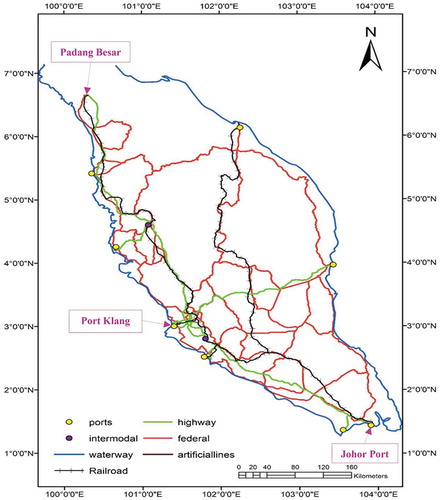
Truck, train and ship are transport vehicles often used for movement of containers, with each having distinct benefits and constraints in terms of time of delivery, economic and environmental matters. The concept of sustainable development in transportation sector has become one of the most influential parameters for policymakers recently (Anderson, Allen, and Browne 2005). In other words, sustainable freight transportation is requisite for timely, cost-efficient and environmental-friendly container movement. Rudi et al. (2017) highlighted that cost and time of transport, and GHG emission are the main criteria to be considered in the design of intermodal transport networks. Hence, this paper is aimed at comparing the results of least-path, road-based, railroad- based and waterway-based optimum routes in terms of transport time, produced emission and transport cost. Furthermore, the study would propose the best route/mode of transport among the alternatives through the integration of SMART approach and sensitivity analysis. For the analyses, two case studies were investigated. The origin and destination points for Case 1 are Johor Port located in south of Peninsular Malaysia, and Padang Besar in the northern part of the transport network, respectively. In Case 2, Johor Port and Port Klang are considered the origin and destination points, respectively. The exact location of origin-destination pairs in the transport network is illustrated in Figure 1.

Figure 1. Origin and destination points for Cases 1 and 2

2. Methodology

2.1. Single-objective decision-making

The transport network of Peninsular Malaysia (Figure 1), which is constructed by using ArcMap, includes ports, intermodal terminals, highways, federal roads, railroads and waterways. Highways have a speed limit of 110 Km/h, while that of federal-roads is 90 Km/h.

The equations for time, emission and cost criteria are presented as Equations 1(1) $Tt=+\mathrm{\Sigma }\left(\frac{td}{sa}\right)+\mathrm{\Sigma }\left(Tmc\right)$(1) , 2(2) $E={\sum }^{}(Ef\times Cw\times Nc\times Td)+{\sum }^{}(Emc),$(2) and 3(3) $\begin{array}{rl}& TC={\sum }^{\hspace{0.17em}}(((Fp\times Fc\times Td)+(Wa\times Tt)+(Ma\times Td))\\ & \times (\frac{Nc}{Cv}))+{\sum }^{\hspace{0.17em}}(0.25\times Tdh\times (\frac{Nc}{Cv}))+{\sum }^{\hspace{0.17em}}(Cmc),\end{array}$(3) , respectively. Transport time was calculated based on the length and speed limit assigned to the links and modal change time. Transport emission (in kg) is a function of emission factor, distance, number of containers and weight of loaded container. Transport cost was estimated based on fuel price, fuel consumption, distance, toll on highway and modal change cost. The total value of each criterion for optimum routes is equal to the sum of the value of each criterion in all involved links plus modal change at ports and intermodal terminals where applicable.

(1) $Tt=+\mathrm{\Sigma }\left(\frac{td}{sa}\right)+\mathrm{\Sigma }\left(Tmc\right)$(1)

where $Tt$ = total transport time (h), $Td$ = transport distance (km), $Sa$ = average speed (km/h) and $Tmc$ = time of modal change (h).

(2) $E={\sum }^{}(Ef\times Cw\times Nc\times Td)+{\sum }^{}(Emc),$(2)

where $E$,$Ef$, $Cw$, $Nc$, $Td$ and $Emc$ are total emission (kg), emission factor (kg/ton-km), container weight (ton), the number of containers, transport distance (km) and emission for modal change (kg). The emission factor for truck, train and ship was obtained from the GHG Protocol (Available at: http://www.ghgprotocol.org/) as 0.08869, 0.0285 and 0.02, respectively. GHG emissions are often expressed in carbon dioxide equivalent (CO₂e), which is based on Global Warming Potential (GWP), by multiplying the amount of the GHG by its GWP. However, in this study, the value of GHG emissions is expressed as CO₂ instead of CO₂e since carbon dioxide was considered as the only emission pollutant and its GWP value is equal to 1.

(3) $\begin{array}{rl}& TC={\sum }^{\hspace{0.17em}}(((Fp\times Fc\times Td)+(Wa\times Tt)+(Ma\times Td))\\ & \times (\frac{Nc}{Cv}))+{\sum }^{\hspace{0.17em}}(0.25\times Tdh\times (\frac{Nc}{Cv}))+{\sum }^{\hspace{0.17em}}(Cmc),\end{array}$(3)

where $TC$ is transport cost (RM), $Fp$ is fuel price (RM/litre), $Fc$ is fuel consumption (litre/km), $Td$ is transport distance (km), $Tdh$ is transport distance on highway (km), $Cmc$ is cost for modal change (RM), $Wa$ is wage (RM/h), $Tt$ is transport time (h), $Ma$ is maintenance (RM/km), $Nc$ is number of containers and $Cv$ represents capacity of the vehicle (number of TEUs). The average toll cost per truck per kilometre was measured as RM 0.25.

The MATLAB software was implemented to design the user-interface and develop the shortest path algorithm to solve the problem in finding optimal path based on different criteria. The detailed method of constructing the transport network, algorithm implementation for the analysis of the network, equations used and assumptions are reported in our previous publication (Gohari et al. 2018). The integration of ArcMap and MATLAB provides a new approach in the analysis of container transport, making it a user-friendly environment for network analysis. The networks were analysed with different values of influential parameters for any pair of origin-destination points for unimodal and intermodal networks.

2.2. Multi-criteria decision-making

The primary aim of multi-criteria decision-making is to propose an ideal route based on the combination of decision criteria. In this study, SMART was integrated with sensitivity analysis. The SMART function model is expressed in Equation (4)(4) $OUp=WAcUPc+WAtUPt+WAeUPe,$(4) .

(4) $OUp=WAcUPc+WAtUPt+WAeUPe,$(4)

where $OUp$ is overall utility assigned to path p, $UPc$, $UPt$ and $UPe$ are utility of path p on attribute cost, utility of path p on attribute time and utility of path p on attribute emission, respectively. $WAc$, $WAt$ and $WAe$ are weight assignment to cost, time and emission, respectively.

The first stage of the analysis entailed the identification of alternatives or options. All minimised routes, which are the results of single-objective analysis, are categorised into 8 and 6 routes for Case 1 and Case 2, respectively. The categorised routes with their associated cost, CO₂ emission and time attributes for Cases 1 and 2 are presented in Tables 1 and 2, respectively. Note that similar routes were categorised in one route number.

$WAcUPc(703.99)+WAtUPt(103.27)=WAcUPc(847.15)+WAtUPt(50.13),$

$WAc0.5+WAt0.00=WAc0.29+WAt1.00,$

$WAt=0.21WAc,$

$WAcUPc(1007.98)+WAeUPe(2769.16)=WAcUPc(1028.33)+WAeUPe(590.26),$

$WAc0.05+WAe0.00=WAc0.02+WAe1.00,$

$WAe=0.03WAc.$

The second step involved the identification of the weights for transportation time (duration), cost and CO₂ emission criteria. The concept of assigning weights involves the categorisation of weights into scaling factors, swing weights, tradeoffs and measure of importance (Merkhofer 2019). The methods for assessing weights are categorised into direct, tradeoff, indirect, ranking (ordinal) and mixed ordinal-cardinal methods (Merkhofer 2019). In tradeoff methods, decision-makers evaluate based on relationships between pairs of weights. The tradeoff method includes methods such as ratio method, tradeoff method and equivalent cost (pricing out) method (Merkhofer 2019). Pricing out is very useful, but requires the definition of performance measures in terms of units familiar to decision-makers with corresponding single-attribute value functions that are linear in those unit. Estimates of equivalent monetary value may then be obtained based on willingness to pay (“How much would you be willing to spend to move the performance measure from its worst level to its best level of performance?”) (Merkhofer 2019). In this study, the cost equivalent method was implemented to assess the tradeoff weights since both the cost attribute and the willingness to pay are in monetary units. In this method, it is required to determine the maximum cost of willingness to pay in order to improve the transport time and CO₂ emission from worst to best performance. For transport time improvement, it was arbitrarily assumed that the maximum cost of willingness to pay is equal to average cost of all the outcomes under consideration which is RM 847.15. For CO₂ emission improvement, the maximum cost of willingness to pay was assumed to be equal to the second highest cost of all the outcomes under consideration which is RM 1028.33. These assumptions in mathematical terms are expressed as:

Table 1. Minimised routes for Case 1

Route		Cost (RM/TEU)	CO2 (kg/TEU)	Time (h)
(1)	Minimum time Highway-based least cost Highway-based least emission	1028.33	1791.96	50.13
(2)	Minimum emission	703.99	590.26	130.27
(3)	Road-based least emission	1020.58	1788.59	50.38
(4)	Minimum cost Railroad-based least time Railroad-based least emission	366.83	627.75	58.76
(5)	Waterway-based least time Waterway-based least emission	806.2	736.84	102.94
(6)	Waterway-based least cost	799.75	752.93	103.99
(7)	Road-based least cost	1007.98	2769.16	51.43
(8)	Federalroad-based least cost Federalroad-based least emission	1043.58	2035.71	57.2

Table 2. Minimised routes for Case 2

Route		Cost (RM/TEU)	CO2 (kg/TEU)	Time (h)
(1)	Minimum time Road-based least emission	719.47	823.3	74.34
(2)	Minimum emission Waterway-based least time Waterway-based least cost	483.62	201.569	83.28
(3)	Minimum cost Railroad-based least time Railroad-based least emission	417.35	291.86	78.39
(4)	Highway-based least emission Highway-based least cost	766.34	919.06	75.22
(5)	Federalroad-based least emission Federalroad-based least cost	734.08	1132.96	77.68
(6)	Road-based least cost	717.63	1424.03	74.61

Finally, the sum of the three attribute weights must equal 1. Therefore,

$WAc+WAe+WAt=1$

$1.24WAc=1$

The weights for the three attributes, $WAc$, $WAt\text{and\ }WAe$, were obtained as 0.806, 0.169 and 0.024, respectively. The same assumptions regarding willingness to pay were considered for Case 2. Thus, the weights for $WAc$, $WAt\text{and\ }WAe$ were obtained as 0.67, 0.3 and 0.03, respectively. The obtained values of criteria weights for both case studies indicate that the most significant factor in shipment considered in this study is cost, followed by time and emission.

In the third stage, the attributes of Tables 1 and 2 were converted proportionately to rankings on a scale of 0 to 1, where 1 and 0 represent the best and worst outcomes, respectively. The result of this conversion for both case studies is presented in Table 3.

Table 3. Ranking of attributes

	Case 1			Case 2
Route	Cost	Emission	Time	Cost	Emission			Time
(1)	7	6	1	4	3			1
(2)	2	1	8	2		1	6
(3)	6	5	2	1		2	5
(4)	1	2	5	6		4	3
(5)	4	3	6	5		5	4
(6)	3	4	7	3		6	2
(7)	5	8	3
(8)	8	7	4

The next stage is to determine the utility value of the criteria weight for all alternatives described in Tables 1 and 2. For this purpose, the criteria were evaluated on a scale of 0 to 1 proportionately using Equation (5)(5) $\begin{array}{rl}& \mathrm{U}\mathrm{t}\mathrm{i}\mathrm{l}\mathrm{i}\mathrm{t}\mathrm{y}\mathrm{v}\mathrm{a}\mathrm{l}\mathrm{u}\mathrm{e}=\\ & \frac{\mathrm{M}\mathrm{a}\mathrm{x}\mathrm{i}\mathrm{m}\mathrm{u}\mathrm{m}\mathrm{v}\mathrm{a}\mathrm{l}\mathrm{u}\mathrm{e}\mathrm{o}\mathrm{f}\mathrm{c}\mathrm{r}\mathrm{i}\mathrm{t}\mathrm{e}\mathrm{r}\mathrm{i}\mathrm{o}\mathrm{n}-\mathrm{v}\mathrm{a}\mathrm{l}\mathrm{u}\mathrm{e}\mathrm{c}\mathrm{r}\mathrm{i}\mathrm{t}\mathrm{e}\mathrm{r}\mathrm{i}\mathrm{o}\mathrm{n}}{\mathrm{M}\mathrm{a}\mathrm{x}\mathrm{i}\mathrm{m}\mathrm{u}\mathrm{m}\mathrm{v}\mathrm{a}\mathrm{l}\mathrm{u}\mathrm{e}\mathrm{o}\mathrm{f}\mathrm{c}\mathrm{r}\mathrm{i}\mathrm{t}\mathrm{e}\mathrm{r}\mathrm{i}\mathrm{o}\mathrm{n}-\mathrm{M}\mathrm{i}\mathrm{n}\mathrm{i}\mathrm{m}\mathrm{u}\mathrm{m}\mathrm{v}\mathrm{a}\mathrm{l}\mathrm{u}\mathrm{e}\mathrm{o}\mathrm{f}\mathrm{c}\mathrm{r}\mathrm{i}\mathrm{t}\mathrm{e}\mathrm{r}\mathrm{i}\mathrm{o}\mathrm{n}}\end{array}$(5) . The utility values for both case studies are presented in Table 4.

(5) $\begin{array}{rl}& \mathrm{U}\mathrm{t}\mathrm{i}\mathrm{l}\mathrm{i}\mathrm{t}\mathrm{y}\mathrm{v}\mathrm{a}\mathrm{l}\mathrm{u}\mathrm{e}=\\ & \frac{\mathrm{M}\mathrm{a}\mathrm{x}\mathrm{i}\mathrm{m}\mathrm{u}\mathrm{m}\mathrm{v}\mathrm{a}\mathrm{l}\mathrm{u}\mathrm{e}\mathrm{o}\mathrm{f}\mathrm{c}\mathrm{r}\mathrm{i}\mathrm{t}\mathrm{e}\mathrm{r}\mathrm{i}\mathrm{o}\mathrm{n}-\mathrm{v}\mathrm{a}\mathrm{l}\mathrm{u}\mathrm{e}\mathrm{c}\mathrm{r}\mathrm{i}\mathrm{t}\mathrm{e}\mathrm{r}\mathrm{i}\mathrm{o}\mathrm{n}}{\mathrm{M}\mathrm{a}\mathrm{x}\mathrm{i}\mathrm{m}\mathrm{u}\mathrm{m}\mathrm{v}\mathrm{a}\mathrm{l}\mathrm{u}\mathrm{e}\mathrm{o}\mathrm{f}\mathrm{c}\mathrm{r}\mathrm{i}\mathrm{t}\mathrm{e}\mathrm{r}\mathrm{i}\mathrm{o}\mathrm{n}-\mathrm{M}\mathrm{i}\mathrm{n}\mathrm{i}\mathrm{m}\mathrm{u}\mathrm{m}\mathrm{v}\mathrm{a}\mathrm{l}\mathrm{u}\mathrm{e}\mathrm{o}\mathrm{f}\mathrm{c}\mathrm{r}\mathrm{i}\mathrm{t}\mathrm{e}\mathrm{r}\mathrm{i}\mathrm{o}\mathrm{n}}\end{array}$(5)

Table 3. Utility values of criteria weight

	Case 1			Case 2
Route	Cost	Emission	Time	Cost	Emission	Time
(1)	0.02	0.44	1.00	0.13	0.49	1.00
(2)	0.5	1.00	0.00	0.81	1.00	0.00
(3)	0.03	0.45	0.99	1.00	0.93	0.55
(4)	1.00	0.98	0.89	0.00	0.41	0.9
(5)	0.35	0.93	0.34	0.1	0.24	0.63
(6)	0.36	0.92	0.32	0.14	0.00	0.97
(7)	0.05	0.00	0.98
(8)	0.00	0.33	0.91

The last step is to compute the overall utility for each alternative. The results of the computations for Case 1 and Case 2 are presented in Tables 4 and 5, respectively. The alternative number 3 and number 4 scored the highest overall utility for Case 1 and Case 2, respectively. Therefore, this is logically the best route to ship one fully loaded 20-foot standard container from the origin to destination.

Table 4. Weighted and overall utility scores and ranking for Case 1

Route	Cost	Emission	Time	Overall utility	Overall rank
(1)	0.016	0.01	0.169	0.195	7
(2)	0.403	0.024	0.00	0.427	2
(3)	0.024	0.01	0.167	0.201	6
(4)	0.806	0.023	0.15	0.979	1
(5)	0.282	0.022	0.057	0.361	4
(6)	0.29	0.022	0.054	0.366	3
(7)	0.04	0.00	0.165	0.205	5
(8)	0.00	0.007	0.153	0.16	8

Table 5. Weighted and overall utility scores and ranking for Case 2

Route	Cost	Emission	Time	Overall utility	Overall rank
(1)	0.09	0.01	0.3	0.4	3
(2)	0.54	0.03	0.00	0.57	2
(3)	0.67	0.028	0.16	0.85	1
(4)	0.00	0.012	0.27	0.28	5
(5)	0.07	0.0007	0.19	0.26	6
(6)	0.1	0.00	0.29	0.39	4

3. Results and discussion

The single-objective decision-making was performed using analyses based on time, emission and cost. The analysis of each criterion includes least path, road-based least path, railroad-based least path and waterway-based least path analyses. The result of least path analysis is the optimum route either through road, railroad or waterway, while the results of road-based, railroad-based and waterway-based analyses are the optimum route using truck, train and ship, respectively.

3.1. Time-based analysis results

The result of least-time analysis is presented in Figure 2. It indicates that using truck can deliver containers sooner than train and ship for both Case 1 and Case 2. The result of the road-based time analysis for both cases is the same as least-time results. The result of railroad-based time analysis for both case studies is shown in Figure 3, while that of waterway-based time analysis is shown in Figures 4 and 5. The result of waterway-based analysis for Case 1 is broken down into two parts since there is no direct waterway route between origin and destination point. The first part of the route was from the start point to node 5, which is the closest node through waterway to the final-destination point with transport time of 66.45 hours. The second part of the route starts from node 5 to the final-destination point, which involves the use of a truck with transport time of 36.49 hours.

Figure 2. Least time analysis for Case 1 (left) and Case 2 (right)

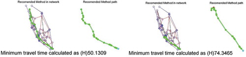
Figure 3. Train-based time analysis for Case 1 (left) and Case 2 (right)

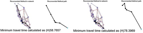
Figure 4. Ship-based time analysis for Case 1 (node 174 to node 5) (left) and (node 5 to node 21) right

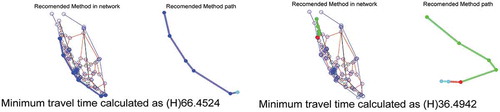
Figure 5. Ship-based time analysis for Case 2

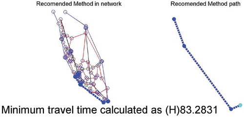
The least-time path analysis was statistically compared with the other transportation modes for both cases, as shown in bar charts of Figure 6. The comparison shows that for both case studies, containers movement by ship is the most time-consuming mode, followed by train and then truck. In Case 1, the movement of containers by using road mode saves approximately 8 and 53 hours compared to railroad and waterway, respectively. In Case 2, movement of containers through roads can deliver containers approximately 4 and 9 hours earlier than railroad and waterway modes, respectively.

Figure 6. Transport time comparison for Case 1 (left) and Case 2 (right)

3.2. Emission-based analysis results

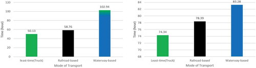
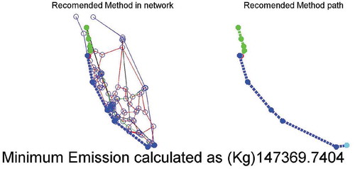
The result of least-emission analysis for both cases is shown in Figure 7. For Case 1, the intermodal transport using ship and train was the best. As for Case 2, transport through only waterway was the best.

Figure 7. Least-emission analysis for Case 1 (left) and Case 2 (right)

The results of road-based emission analysis for Cases 1 and 2 are depicted in Figure 8. Since there are available highway and federal road alternatives for both cases, both highway-based and federal road-based emission analyses were performed. The results of highway-based emission analysis for Cases 1 and 2 are depicted in Figure 9, while the results of federal road-based emission analysis for Cases 1 and 2 are shown in Figures 10 and 11, respectively. For Case 2, the total emission of federal-road-based route consists of emissions from loading containers onto the truck at origin, transport through federal road to the closest intersection point between federal road and highway to the destination point, transport through highway to the final destination and unloading containers from the truck at destination. This breakdown is due to the absence of a federal road connected to the destination node. The total transport emissions for Case 1 and Case 2 were estimated at 407.142 ton and 226.593 ton, respectively.

Figure 8. Truck-based emission analysis for Case 1 (left) and Case 2 (right)

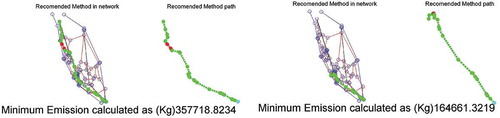
Figure 9. Highway-based emission analysis for Cases 1 (left) and Case 2 (right)

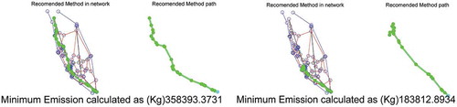
Figure 10. Federal-road-based emission analysis for Case 1

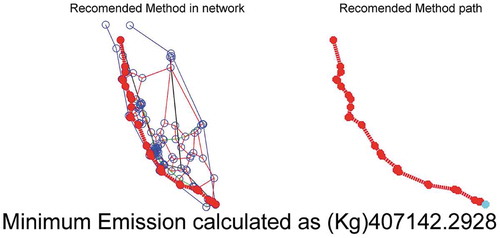
Figure 11. Federal-road-based emission analysis for Case 2

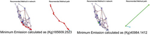
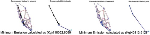
The results of railroad-based emission analysis for both cases are depicted in Figure 12. The result of waterway-based emission analysis for Case 1 is illustrated in Figure 13. The result of waterway-based emission analysis for Case 2 is similar to that of least-emission analysis for Case 2 (Figure 7).

Figure 12. Train-based emission analysis for Case 1 (left) and Case 2 (right)

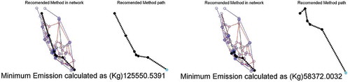
Figure 13. Ship-based emission analysis for Case 1

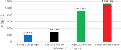
The least-emission path was compared with the other transportation modes for Cases 1 and 2, as depicted with bar charts in Figures 14 and 15, respectively. For Case 1, the movement of containers through intermodal transport by combined usage of ship and train emitted the least emission (waterway-railway modes), followed by train, ship–truck combination, truck by highway and truck by federal road. From Figure 14, the combination of waterway–railway modes can transport each container with less CO₂ emission of approximately 37.5, 146.5, 1201.7 and 1445.4 kg than railroad, waterway, highway and federal road routes, respectively. In Case 2, the destination point is not connected to the federal road network. Therefore, the federal road-based route includes federal road for majority of the path and highway for a small portion of the path, which are represented by red and green colours, respectively (Figure 15). The comparison for Case 2 clearly indicated that the movement of containers by ship was the most environmental-friendly mode, followed by train, truck by highway and truck by federal road. The CO₂ emission per TEU of federal road and highway was about 931.4 and 717.5 kg higher than waterway, respectively. In addition, train emitted 90.3 kg of CO₂ more than ship for movement of each container. In general, highway-based and federal road-based routes, respectively, emitted about 5.6- and 4.5-times higher CO₂ than the waterway mode.

Figure 14. Transport emission comparison for Case 1

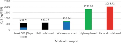
Figure 15. Transport emission comparison for Case 2

The results show that container transport by utilising ship–train combination and ship produced the lowest possible CO₂ emissions for Cases 1 and 2, respectively, while movement via truck produced considerably higher CO₂ emission compared to ship and train for both Cases. Particularly in Case 1, although waterway-based route involves a mode-to-mode transfer, its CO₂ emission was noticeably lower than truck mode for both highway and federal road (i.e. highway and federal road emitted CO₂ of about 2.4 and 2.7 times more than waterway).

3.3. Cost-based analysis result

The results of the least-cost analysis for both cases are illustrated in Figure 16. The results clearly show that transport by train is the cheapest mode of transport for both Cases. The results of the road-based and highway-based cost analyses for Cases 1 and 2 are illustrated in Figures 17 and 18, respectively. The result of federal road-based cost analysis for Cases 1 and 2 are depicted in Figures 19 and 20, respectively. The total transport costs for Cases 1 and 2 were calculated as RM 208,716.87 and RM 146,816.47, respectively. For Case 2, the federal road-based route consists of the cost of loading containers onto truck at origin, transport cost through federal road to the closest intersection point between federal road and highway to the destination point, and transport cost through highway to the final destination plus cost of unloading containers from truck at the destination.

Figure 16. Least-cost analysis for Case 1 (left) and Case 2 (right)

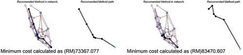
Figure 17. Truck-based cost analysis for Case 1 (left) and Case 2 (right)

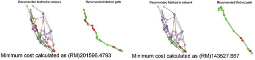
Figure 18. Highway-based cost analysis for Case 1 (left) and Case 2 (right)

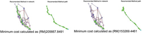
Figure 19. Federal-road-based cost analysis for Case 1

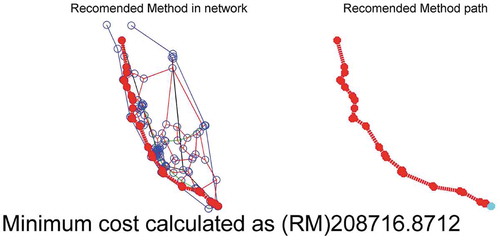
Figure 20. Federal-road-based cost analysis for Case 2

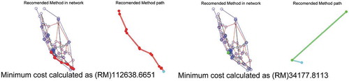
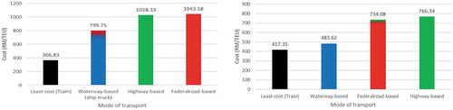
The results of railroad-based cost analysis are the same as least-cost analysis (Figure 16), and the results of waterway-based cost analysis for both cases are illustrated in Figure 21. The least-cost path was compared with the other transportation modes and these comparisons are shown as bar charts in Figure 22 for both cases. The comparison for Cases 1 and 2 clearly indicates that train mode was the cheapest mode of transport, followed by the waterway and road mode. For Case 2, waterway-based, road-based, federal road-based and highway-based routes exhibit higher transport costs approximately by 15%, 72%, 75% and 83%, respectively, for each container when compared with railroad mode. Similarly, transport costs of waterway-based, road-based, federal road-based and highway-based routes in Case 1 were about 72%, 174%, 184% and 180% higher, respectively, compared with railroad mode for each container. The results for both case studies showed that transport of containers by truck was the costliest, especially in Case 1. Although waterway-based route includes one mode-to-mode transfer, its cost was lower than truck mode (road-based, highway-based and federal road-based routes).

Figure 21. Ship-based cost analysis for Case 1 (left) and Case 2 (right)

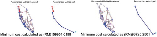
Figure 22. Transport cost comparison for Case 1 (left) and Case 2 (right)

3.4. Results of sensitivity analysis for both Case studies

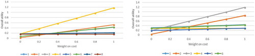
The sensitivity analysis of the weighting assessment was performed to investigate how the best route is affected by varying the weights of time, CO₂ emission and cost. The analysis was executed by varying the weight of one attribute while keeping all other attributes constant. The results of the analysis for both cases based on the weights of time, CO₂ emission and cost are presented in Figure 23, 24 and 25, respectively. The sensitivity analysis for Case 1 indicates that routes in category number 4 (railroad mode) are the most preferred options as the weight of all attributes are increased. For Case 2, it is clearly seen that route 3, which is the least-cost route, becomes the preferred option as the weight of all attributes is increased.

Figure 23. Sensitivity analysis by increasing weight of time for Case 1 (left) and Case 2 (right)

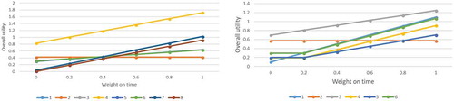
Figure 24. Sensitivity analysis by increasing weight of CO₂ emission for Case 1 (left) and Case 2 (right)

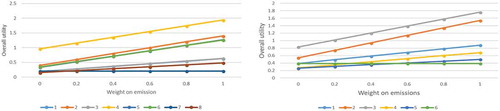
Figure 25. Sensitivity analysis by increasing weight of cost for Case 1 (left) and Case 2 (right)

4. Conclusion

This paper presents the results of single-objective route/modal choice analyses for two case studies in transport network of Peninsular Malaysia. Four different analyses were performed: least path, road-based, railroad-based and waterway-based least path analyses, based on time, emission and cost. The outcomes of both cases were compared to understand the differences in terms of considered criteria. Comparing the result of time-based analyses indicated that the trucks are faster than trains and ships. In terms of CO₂ emission, transport by ship is the most environmental-friendly mode of transport. The transport of containers using train was the cheapest followed by ship and truck. For multi-criteria analyses, the SMART integrated with the sensitivity analysis was implemented to select the best route/mode of transport among the alternatives obtained from single-objective analysis to meet the combination of all criteria. The analyses revealed that, although the transport of containers via train is not as fast as trucks, and has more CO₂ emission than ships, it is an ideal transport mode when the criteria are combined. Therefore, it is suggested that stakeholders in the transport sector should invest in improving railway infrastructure for the possible use of higher speed trains and modern trains that produce less amount of emissions. This will enhance the timely delivery of local containers with less air pollution and reduction in final price of goods.

Furthermore, future research should consider the implementation of a variety of statistical and computational methods such as goal programming, AHP and epsilon constraint approaches to comprehensively explore container transport modes and provide better comparative analyses. Moreover, route/modal choices under different scenarios of criteria weights such as assigning higher weight value to emission or time criteria than cost need to be evaluated. In addition, comparison of unimodal and intermodal transportations of containers in terms of external cost of transport should be considered.

Disclosure statement

No potential conflict of interest was reported by the authors.

Correction Statement

This article has been republished with minor changes. These changes do not impact the academic content of the article.

Additional information

Notes on contributors

Adel Gohari

Adel Gohari is a Research Officer at the Civil and Environmental Engineering Department of Universiti Teknologi PETRONAS (UTP). He has graduated from Ph.D. and Master’s degree in Civil Engineering (Transportation and Highway Engineering) and Geoinformatics from the Universiti Teknologi PETRONAS (UTP) and Universiti Teknologi Malaysia (UTM) in 2018 and 2011, respectively. He is so enthusiastic in research activities mainly in the fields of Transportation Engineering, Geographic Information System (GIS), and the application of Multi-Criteria Decision Analysis (MCDA) in different disciplines.

Ali Tighnavard Balasbaneh

Ali Tighnavard Balasbaneh is a lecturer at Universiti Tun Hussein Onn Malaysia (UTHM). He received his Ph.D. in civil engineering (construction management) in 2014 from the Universiti Teknologi Malaysia. His research interests cover several aspects of sustainability with a special focus on multi-criteria decision making. He teaches different subjects in construction management such as sustainability and environment. He also organized workshops on life cycle assessment of products and materials for academics and professionals.

Khamaruzaman W. Yusof

Khamaruzaman W. Yusof is an Associate Professor and lecturer at the Civil and Environmental Engineering Department of Universiti Teknologi PETRONAS (UTP) since 2011. He has graduated from Ph.D. degree in 2001 from the Coventry University, United Kingdom. His major fields of expertise are Geographic Information System (GIS), Remote Sensing (RS), and water resources.Iraj Toloue is a post-doctoral candidate at the Civil and Environmental Engineering Department of Universiti Teknologi PETRONAS (UTP) where he accomplished his Ph.D. studies. His expertise is in the field of Structural Analysis. However, he has sound knowledge of MATLAB programming and its applications in a wide area of Civil Engineering including Transportation Engineering. 

Iraj Toloue

Iraj Toloue is a post-doctoral candidate at the Civil and Environmental Engineering Department of Universiti Teknologi PETRONAS (UTP) where he accomplished his Ph.D. studies. His expertise is in the field of Structural Analysis. However, he has sound knowledge of MATLAB programming and its applications in a wide area of Civil Engineering including Transportation Engineering.

Abdulkadir Taofeeq Sholagberu

Abdulkadir Taofeeq Sholagberu is a lecturer at the Department of Water Resources & Environmental Engineering, University of Ilorin, Nigeria. He has completed the Ph.D. studies at the Civil and Environmental Engineering Department of Universiti Teknologi PETRONAS in 2019. The area of his research interests includes Water Resources, Transportation studies, and Soil Erosion.

Razi Hasan

Razi Hasan is pursuing his PhD at the Centre for Accident Research and Road Safety − Queensland (CARRS-Q). His research aims to yield better results from the Roadside Drug Testing program (RDT) by improving drug driving deterrence at both general and specific levels. His research and experience cover several areas including road safety, pedestrian safety and road infrastructure design.

References

- Anderson, S., J. Allen, and M. Browne. 2005. “Urban Logistics – How Can It Meet Policy Makers’ Sustainability Objectives?” Journal of Transport Geography 13 (1): 71–81. doi:https://doi.org/10.1016/j.jtrangeo.2004.11.002.
- Barfod, M. B., and S. Leleur. 2014. Multi-criteria Decision Analysis for Use in Transport Decision Making. 2 ed. DTU Lyngby: Technical University of Denmark, Transport.
- Bergqvist, R., C. Macharis, D. Meers, and J. Woxenius. 2015. “Making Hinterland Transport More Sustainable a Multi Actor Multi Criteria Analysis.” Research in Transportation Business & Management 14: 80–89. doi:https://doi.org/10.1016/j.rtbm.2014.10.009.
- Chen, S. L., J. Jeevan, and S. Cahoon. 2016. “Malaysian Container Seaport-hinterland Connectivity: Status, Challenges and Strategies.” The Asian Journal of Shipping and Logistics 32 (3): 127–138. doi:https://doi.org/10.1016/j.ajsl.2016.09.001.
- Demir, E., M. Hrusovsky, W. Jammernegg, and T. Van Woensel. 2019. “Green Intermodal Freight Transportation: Bi-objective Modelling and Analysis.” International J of Production Research 57(19): 6162-6180 https://doi.org/10.1080/00207543.2019.1620363.
- Department of Statistics Malaysia. “External Trade.” http://www.statistics.gov.my/index.php?r=column/ctimeseriesandmenu_id=NHJlaGc2Rlg4ZXlGTjh1SU1kaWY5UT09
- Gajanand, M. S., and T. T. Narendran. 2013. “Green Route Planning to Reduce the Environmental Impact of Distribution.” International Journal of Logistics Research and Applications 16 (5): 410–432. doi:https://doi.org/10.1080/13675567.2013.831400.
- Gohari, A., A. N. Matori, K. W. Yusof, I. Toloue, K. C. Myint, and A. T. Sholagberu. 2018. “Route/Modal Choice Analysis and Tradeoffs Evaluation of the Intermodal Transport Network of Peninsular Malaysia.” Cogent Engineering 5: 1. doi:https://doi.org/10.1080/23311916.2018.1436948.
- Hamurcu, M., and T. Eren. 2019. “An Application of Multicriteria Decision-making for the Evaluation of Alternative Monorail Routes.” Mathematics 7 (1): 16. doi:https://doi.org/10.3390/math7010016.
- Kumru, M., and P. Y. Kumru. 2014. “Analytic Hierarchy Process Application in Selecting the Mode of Transport for a Logistics Company.” Journal of Advanced Transportation 48 (8): 974–999. doi:https://doi.org/10.1002/atr.1240.
- Lam, J. S. L., and Y. Gu. 2016. “A Market-oriented Approach for Intermodal Network Optimisation Meeting Cost, Time and Environmental Requirements.” International Journal of Production Economics 171: 266–274. doi:https://doi.org/10.1016/j.ijpe.2015.09.024.
- Laurent, A. B., S. Vallerand, Y. Van der Meer, and S. D’amours. 2020. “CarbonRoadMap: A Multicriteria Decision Tool for Multimodal Transportation.” International J of Sustainable Transportation 14(3): 205-214. https://doi.org/10.1080/15568318.2018.1540734.
- Lee, C. Y., and D. P. Song. 2017. “Ocean Container Transport in Global Supply Chains: Overview and Research Opportunities.” Transportation Research Part B: Methodological 95: 442–474. doi:https://doi.org/10.1016/j.trb.2016.05.001.
- Machari, C., D. Meers, and T. V. Lier. 2015. “Modal Choice in Freight Transport: Combining Multi-criteria Decision Analysis and Geographic Information Systems.” International Journal of Multicriteria Decision Making 5 (4): 355–371. doi:https://doi.org/10.1504/IJMCDM.2015.074087.
- Macharis, C., A. De Witte, and J. Ampe. 2009. “The Multi-actor, Multi-criteria Analysis Methodology (MAMCA) for the Evaluation of Transport Projects: Theory and Practice.” Journal of Advanced Transportation 43 (2): 183–202. doi:https://doi.org/10.1002/atr.5670430206.
- Merkhofer, M. W. 2019. “Choosing the Wrong Portfolio of Projects: 6 Reasons Organizations Choose the Wrong Projects (And What to Do about It).” https://www.prioritysystem.com/reasons4i.html
- Monprapussom, S., D. Thaitakoo, D. J. Watts, and R. Banomyong. 2009. “Multi Criteria Decision Analysis and Geographic Information System Framework for Hazardous Waste Transport Sustainability.” Journal of Applied Sciences 9 (2): 268–277. doi:https://doi.org/10.3923/jas.2009.268.277.
- Motos. 2007. “Transport Modelling: Towards Operational Standards in Europe, E, CTT, DTU, TREN/06/FP6SSP/S07.56151/022670.”
- Nasir, S. 2014. “Intermodal Container Transport Logistics to and from Malaysian Ports: Evaluation of Customer Requirements and Environmental Effects.” PhD diss., KTH Royal Institute of Technology.
- Oh, T. H., and S. C. Chua. 2010. “Energy Efficiency and Carbon Trading Potential in Malaysia.” Renewable and Sustainable Energy Reviews 14 (7): 2095–2103. doi:https://doi.org/10.1016/j.rser.2010.03.029.
- Ong, H. C., T. M. I. Mahlia, and H. H. Masjuki. 2012. “A Review on Energy Pattern and Policy for Transportation Sector in Malaysia.” Renewable and Sustainable Energy Reviews 16 (1): 532–542. doi:https://doi.org/10.1016/j.rser.2011.08.019.
- Pechanec, V. 2013. Analýza Krajiny Prostřednictvím SDSS, 173. Habilitační práce, Brno: Mendelova univerzita.
- Rudi, A., M. Frohling, K. Zimmer, and F. Schultmann. 2017. “Freight Transportation Planning considering Carbon Emissions and In-transit Holding Costs: A Capacitated Multi-commodity Network Flow Model.” EURO Journal on Transportation and Logistics 5 (2): 123–160. doi:https://doi.org/10.1007/s13676-014-0062-4.
- Sawadogo, M., and D. Anciaux 2010. “Reducing the Environmental Impacts of Intermodal Transportation: A Multi-criteria Analysis Based on ELECTRE and AHP Methods.” In 3rd International Conference on Information Systems, Logistics and Supply Chain Creating value through green supply chains, Casablanca, Morocco, 224. April.
- Stoilova, S. 2018. “Evaluation Efficiency of Intermodal Transport Using Multi-criteria Analysis.” In Proceedings of 17th International Scientific Conference Engineering for Rural Development, Jelgava, Latvia, 2030–2039.
- United Nations Economic and Social Commision For Asia and The Pacific. 2007. “Regional Shipping and Port Development: Container Traffic Forecast 2007 Update.”